Updated Lagrangian Particle Hydrodynamics (ULPH) Modeling of Natural Convection Problems

1  Introduction

Natural convection has extensive applications across natural phenomena and engineering domains. It is pivotal in various heat transfer and fluid mechanics scenarios, such as ventilation within buildings, heat exchange in air conditioning systems, and cooling processes in nuclear reactors, and it has been gaining significant attention in the research literature. Genuine natural convection involves complex fluid dynamics phenomena, including nonlinear, non-stationary, and multiscale features. It typically occurs in systems with complex geometric shapes and boundary conditions. Due to these complexities, accurately simulating natural convection problems is challenging. Therefore, robust and accurate numerical methods are required to predict and understand natural convection behavior.

Many numerical methodologies have been proposed for exploring heat transfer through natural convection in various geometries. Khanafer et al. [1] utilized the finite volume method (FVM) to investigate the enhancement of buoyancy-driven heat transfer within a two-dimensional enclosure. Within a circular-wavy cavity, Hatami et al. [2] obtained reliable results for natural convection problems using the finite element method (FEM). The same study was conducted by Liang et al. [3] using the meshless using meshless moving particle semi-implicit method (MPS). Kuehn et al. [4] simulated natural convection in concentric cylinders using the finite difference method (FDM). The same geometry was also modelled by Sheikholeslami et al. [5] using the lattice Boltzmann method (LBM) and Yang et al. [6] using the smoothed particle hydrodynamics (SPH) method. Primarily due to their geometric simplicity, benchmark solutions for some simple geometry problems have been widely explored and referenced [7,8].

The SPH method has been widely used in natural convection as a commonly used meshless method. Chaniotis et al. [9] used a re-meshing procedure in SPH to simulate natural convection problems and achieved excellent accuracy. To deal with natural convection which involves a significant change in density with temperature, Szewc et al. [10] used the SPH method to investigat natural convection with a non-Boussinesq formulation. Aly [11] used the stabilized incompressible smoothed particle hydrodynamics (ISPH) method to model natural convection at different Rayleigh numbers (103 ≤ Ra ≤ 105) in 2D and 3D square cavities. Ng et al. [12] utilized the Adami approach in SPH to simulate Dirichlet temperature boundary conditions for arbitrarily shaped geometries, studying natural convection problems with complex boundaries. Yang et al. [13] simulated natural convection at high Rayleigh numbers using the δ-SPH method, incorporating kernel gradient correction (KGC) technique and particle shifting technology (PST). Li et al. [14] developed an integrated SPH method incorporating advanced techniques such as artificial viscosity, KGC, boundary treatment, and others, successfully obtaining more stable results in simulating natural convection.

Recently, Tu et al. proposed a novel meshless method named updated Lagrangian particle hydrodynamics (ULPH) [15]. ULPH draws inspiration from peridynamics (PD) and SPH methodologies. Similarly, the general particle dynamics (GPD) method proposed by Yao et al. [16] and the updated Lagrangian nonlocal general particle dynamics (UL-NGPD) method proposed by Yin et al. [17] were developed, inspired by PD and SPH, primarily to solve problems involving large elastic-plastic deformations in solids. ULPH is essentially a fluid version of PD and thus has the potential to be combined with PD to investigate complex engineering fluid-solid coupling problems. Additionally, as a Lagrangian meshless method, ULPH has drawn on insights from SPH [18]. In the ULPH method, the Navier-Stokes equation is solved by nonlocal differential operators. With the emergence of the high-order ULPH theory proposed by Yan et al. [19], nonlocal differential operators can meet the requirements of any order of accuracy. As a result, ULPH exhibits superior accuracy. However, the ULPH method has not yet been extensively applied to investigate natural convection problems. Given its high accuracy, good convergence, and stability advantages, this method holds promise for advancing the study of natural convection problems.

This work aims to establish a non-isothermal buoyancy fluid model based on ULPH and apply it to complex natural convection problems. The foundational equations for natural convection will be set up for this model using differential operators. Given the requirement to solve the Laplacian operator for temperature in the energy equation, the second derivatives of temperature can be directly solved using ULPH higher-order theory. It demonstrates the advantage of the ULPH method, enhancing computational accuracy. Due to its characteristics as a Lagrangian method, ULPH can adeptly simulate natural convective fluid flows by directly tracing particles.

The arrangement of this manuscript unfolds as follows: Section 2 delineates the governing equations for weakly compressible fluids and elucidates the fundamental theories of the ULPH method. Additionally, it outlines the heat transfer equations pertinent to the ULPH framework for non-isothermal buoyant fluids. In Section 3, several examples are used to verify the effectiveness and accuracy of the proposed method in simulating natural convection. The numerical results are compared against available numerical solutions in the literature. Conclusions are presented in Section 4.

2  Methodology

2.1 Governing Equations for Weakly Compressible Fluid

In natural convection, density changes induced by temperature are typically approximated by the Boussinesq approximation, often expressed as a change in gravity rather than buoyancy. The Lagrangian formulation for governing equations in viscous flow with natural convection heat transfer [12] can be expressed as follows:

Continuity equation:

DρDt=−ρ∇⋅v,(1)

where ρ denotes density, and v is the velocity of particles.

Momentum equation:

DvDt=−1ρ∇p+μρ∇2v−βg(T−T0),(2)

where μ represents the fluid dynamic viscosity, β is the coefficient of thermal expansion, and g denotes the gravitational acceleration. Similarly, T represents the current temperature, and T0 is the initial temperature of the fluid.

Energy equation:

CpDTDt=κρ∇2T,(3)

where Cp is the specific heat capacity of the fluid, and κ is the coefficient of heat conductivity.

In this work, fluid is considered weakly compressible [20]. In order to fulfill the weakly compressible condition, the Mach number (Ma) must be controlled as follows:

Ma=‖v‖c0≤0.1,(4)

where c0 is a manually set sound speed, not the actual sound speed in the fluid. From Eq. (4), c0 must adhere to the following condition:

c0≥10max(‖v‖).(5)

We use the linear equation of state [21,22] to calculate pressure (p), which is assumed to have the following relation:

p=c02(ρ−ρ0),(6)

where ρ is the current density of particles and ρ0 is the initial density of the fluid.

2.2 Nonlocal Differential Operators

The commonly used ULPH method employs first-order nonlocal differential operators with only first-order accuracy. However, in Eqs. (2) and (3), second-order derivatives are needed to compute the Laplace operator. Therefore, the formulation of second-order nonlocal differential operators is presented in this section using a two-dimensional quadratic polynomial basis. According to the higher-order nonlocal theory of ULPH by Yan et al. [19], the first-order and second-order derivatives of the two-dimensional function u(x) based on quadratic polynomial basis q(x) is obtained as follows:

[∂u(x1, x2)∂x1∂u(x1, x2)∂x2∂2u(x1, x2)∂x12∂2u(x1, x2)∂x1∂x2∂2u(x1, x2)∂x22]=(1000001000002000001000002)M−1(xI)∑J=1Nω(xIJ)q(xIJ)(u(xJ)−u(xI))VJ,(7)

where the two scalars x1 and x2 are used to represent the vector x. Therefor u(x) can be represented as u(x1, x2). M(x) is the shape tensor which has the following expression [15]:

M(xI)=∑J=1Nω(xIJ)q(xIJ)qT(xIJ)VJ,(8)

where xIJ=xJ−xI, and particle J is the family member of particle I. VJ is the volume of particle J. q(xIJ) is the quadratic polynomial basis which can be expressed through the following relation:

q(xIJ)=[(x1J−x1I), (x2J−x2I), (x1J−x1I)2, (x1J−x1I)(x2J−x2I), (x2J−x2I)2]5×1T.(9)

Eq. (9) can be simplified as follows:

q(xIJ)=[dx1, dx2, (dx1)2, (dx1)(dx2), (dx2)2]5×1T.(10)

ω(xIJ) is the kernel function. In this work, we choose the improved Gaussian kernel function as ω(xIJ), with its expression:

ω(r, h)=αd(e−(r/h)2−C), r≤δ,(11)

where r = |x′− x| represents the distance between the particles, and h is the smoothing length, typically set to 1.2 times the initial distance between particles, known as the grid size. δ represents the support domain radius of point x. Subscript d represents the spatial dimension: d = 2 for two dimensions and d = 3 for three dimensions. C is a constant with a value equal to e−9. The expression for normalization coefficient αd is defined as:

αd=1hdπd/2(1−10e−9).(12)

From Eq. (7), we can obtain the gradient operator, divergence operator, and Laplacian operator of the field function u(x) as follows:

{∇uI=∑J=1Nω(xJ−xI)(u(xJ)−u(xI))⊗((1000001000)M−1(xI)q(xJ−xI))VJ∇⋅uI=∑J=1Nω(xJ−xI)(u(xJ)−u(xI))⋅((1000001000)M−1(xI)q(xJ−xI))VJ∇2uI=∑J=1Nω(xJ−xI)(u(xJ)−u(xI))⋅((0020000002)M−1(xI)q(xJ−xI))VJ.(13)

Eq. (13) can be written as follows in its general form using (∙) to denote an arbitrary vector field:

{∇I⊗(∙):=∑J=1Nω(xIJ)(Δ(∙))⊗(B1MI−1q(xIJ))VJ∇I⋅(∙):=∑J=1Nω(xIJ)(Δ(∙))⋅(B1MI−1q(xIJ))VJ∇I2(∙):=∑J=1Nω(xIJ)(Δ(∙))⋅(B2MI−1q(xIJ))VJMI=∑J=1Nω(xIJ)q(xIJ)qT(xIJ)VJ,(14)

where Δ(∙):=(∙)J−(∙)I. The matrices B1 and B2 can be expressed as follows:

B1=(1000001000),B2=(0020000002).(15)

2.3 ULPH Scheme for Natural Convection Problem

Using the second-order nonlocal differential operators in Eq. (14) is feasible to solve Navier-Stokes equations. The continuity equation can be transformed into discrete form using nonlocal divergence operators given below:

DρIDt=−ρI∑J=1Nω(xIJ)Δv⋅(B1MI−1q(xIJ))mJρJ,(16)

where Δv=vJ−vI represents the difference in velocities. Moreover, mJρJ=VJ is considered as the volume of each particle in the neighborhood.

For momentum equation given in Eq. (2), ∇p and ∇2v can be denoted separately as in the following equations:

∇p=∑J=1Nω(xIJ)(Δp)⊗(B1MI−1q(xIJ))mJρJ,(17)

∇2v=∑J=1Nω(xIJ)(Δv)⋅(B2MI−1q(xIJ))mJρJ.(18)

Then, the discrete form of the ULPH momentum equation takes the following form:

DvIDt=1ρI[−∑J=1Nω(xIJ)(Δp)⊗(B1MI−1q(xIJ))mJρJ+∑J=1Nω(xIJ)(Δv)⋅(B2MI−1q(xIJ))mJρJ]−βg(T−T0).(19)

The following expression can also be obtained for the momentum equation:

DTDt=κρ⋅cρ∑J=1Nω(xIJ)ΔT⋅(B2MI−1q(xIJ))mJρJ.(20)

2.4 Boundary Conditions

Particles near the boundary have incomplete neighborhoods, which may lead to non-physical responses, lower accuracy in calculation results, and even computational errors. Therefore, additional processing of the boundaries is necessary. This study employs fixed boundary dummy particles [23]. We apply three layers of fixed dummy particles to ensure that neighborhoods of particles near the boundaries remain intact and prevent particles from penetrating the boundaries.

Fluid particles move over time, while the positions of boundary virtual particles remain fixed. The physical information of boundary particles is computed based on fluid particles within the support domain of these boundary particles. Free-slip or no-slip boundary conditions can be applied to virtual particles at the boundary. The velocity of the boundary virtual particles is determined as follows when applying a no-slip boundary condition:

vw=2vi−v~i,(21)

where vi is regarded as the preset boundary velocity. Similarly, v~i is denoted in the following expression:

v~i=∑jNvjωij∑jNωij,(22)

where i stands for the dummy boundary particles. Moreover, j refers to the neighboring fluid particle adjacent to particle i.

Likewise, the neighboring fluid particles determine the pressure of boundary particles pi according to the following relation:

pi=∑jNpjωij−(βg(T−T0)+ai)⋅∑fρfxijωij∑jNωij,(23)

where pj is the pressure of neighboring fluid particles. ai is the prescribed acceleration of the solid boundary while ai = 0 is used for the fixed solid boundary condition.

For the boundary temperature, a fixed temperature can be set for a thermostatic boundary. For adiabatic boundaries, the temperature is calculated as follows:

Ti=∑jNTjωij∑jNωij.(24)

3  Numerical Verifications

The convergence of second-order nonlocal differential operators was first examined to evaluate the capability of the ULPH method. Then, several benchmark cases were used to demonstrate the effectiveness of the ULPH natural convection model. Comparisons were made between the ULPH results and other numerical solutions.

3.1 Accuracy and Convergence

A mathematical function was selected for testing to validate the accuracy and convergence of the method. Using the second-order nonlocal differential operators within the ULPH method, the first and second derivatives were calculated and compared with analytical solutions. We selected the following hyperbolic cosine function for validation:

f(x, y)=cosh⁡(x2+y22).(25)

with the computational domain is (x, y)∈[−1,1]×[−1,1].

The computational domain was discretized using 441 to 251,001 particles, employing either uniform or non-uniform distributions, as illustrated in Fig. 1. The non-uniform distribution is achieved based on the uniform distribution. For each particle in the uniform distribution, we know its coordinate position and the particle spacing dp. Then we can generate two random numbers dx and dy. And the range of these two random numbers is between −0.5 and 0.5dp. That is, the position of the particle changes from (x, y) to (x + dx, y + dy). To account for the boundaries of the model, three additional layers of boundary particles were incorporated into the computational domain. These boundary particles ensure the completeness of the support domain for particles near the boundaries.

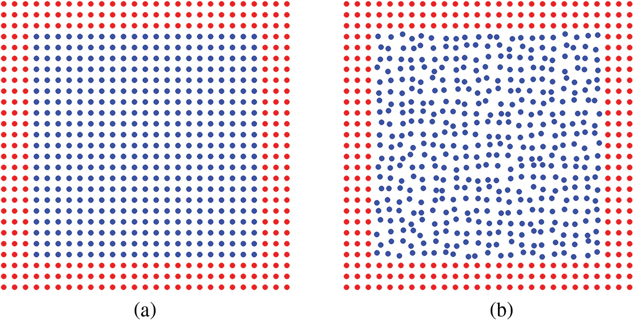
Figure 1: Particle distribution: (a) uniform distribution, (b) non-uniform distribution

Root mean square error (RMSE) was used to measure the convergence speed [24], defined by the following formula:

RMSE(f)=[∑J=1N1N(fJpredicted−fJexact)2]0.5,(26)

where N represents the total amount of particles, excluding boundary particles. Moreover, fpredicted denotes the numerical solution of the calculation while fexact represents the analytical solution of the function.

Fig. 2a,b shows the relationship between the RMSE for the first derivatives of the function and the total number of particles. Both uniform and non-uniform distributions show good convergence. The distribution of particles does not significantly affect the accuracy of the first derivatives, as the results of the two distribution methods are essentially consistent. Fig. 2c–e shows the convergence of the second derivatives of the function. While the non-uniform distribution has a significant impact, the accuracy of the second derivative still improves with an increase in the total number of particles. It demonstrates the computational ability of the ULPH method to solve second-order derivative problems.

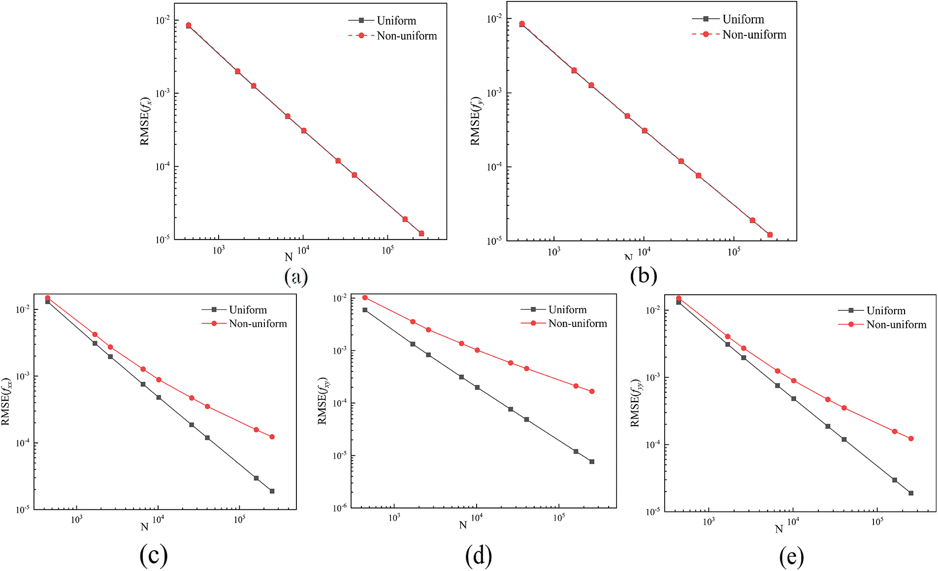
Figure 2: The RMSE of the first and second derivatives of f(x, y): (a) fx, (b) fy, (c) fxx, (d) fxy, (e) fyy

3.2 Natural Convection in a Square Cavity

Firstly, we considered a classic two-dimensional benchmark for natural convection in a square cavity, as shown in Fig. 3. The specific parameters for simulation are as follows. The length of the cavity L = 1.0 m, with an initial density ρ0 = 1.0 kg/m3. In addition, the viscosity coefficient μ = 10−5 Pa·s, the thermal conductivity k = 0.01 W/(m⋅K), the specific heat capacity of the fluid Cp = 710 J/(kg⋅K), and the fluid thermal expansion coefficient β = 0.00140845 K−1. The left and the right walls were fixed at temperatures Th and Tc, respectively. The horizontal boundaries at the top and bottom were adiabatic. The initial temperature of the fluid was taken as T0. The gravitational acceleration g = 10 m/s2 in the negative y-axis direction. All walls were set to no-slip boundary conditions.

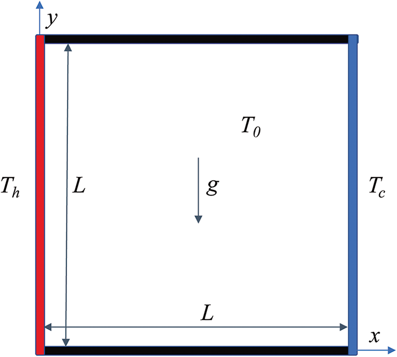
Figure 3: Schematic diagram of the two-dimensional square cavity

The following dimensionless parameters were used to describe the model:

X=xL,Y=yL,Vx=uLα,Vy=vLα,andT∗=T−TCTH−TC.(27)

Moreover, the thermal diffusion coefficient is defined in the following manner:

α=κρCp.(28)

For natural convection, the flow characteristics are mainly related to two dimensionless quantities, Rayleigh number (Ra) and Prandtl number (Pr), which are defined as shown below:

Ra=ρ02CpgβΔTL3kμ,(29)

Pr=μCpk.(30)

In this case, except for temperature, all other parameters have been determined. The Rayleigh number is controlled by ΔT. The initial fluid temperature was set as T0 = 300 K. After that, the temperatures of hot and cold walls were calculated by Th = T0 + ΔT/2 and Tc = T0 −ΔT/2, respectively. We simulated natural convection for Rayleigh numbers Ra = 103, 104, and 105, corresponding to ΔT =10−5, 10−4, and 10−3 K, respectively.

Fig. 4a–f displays the snapshots of temperature distribution from initial to steady state under the condition of Ra = 105. As shown in Fig. 4a, heat conduction dominated at the boundaries with hot and cold walls during the initial heat transfer period. At the time t = 250 s, illustrated in Fig. 4c, the fluid near the adiabatic boundaries exhibited a noticeably asymmetric temperature distribution, indicating the onset of convective phenomena. At t = 3000 s, demonstrated in Fig. 4f, the temperature field of the fluid reached a steady state with a symmetric temperature distribution. A significant temperature gradient along the horizontal direction was evident near the adiabatic boundaries caused by the heat flux vector in the same direction. Analyzing this with Eq. (2) reveals the movement mechanism. The fluid near the hot wall warms up, resulting in a buoyancy force opposite to gravity, causing upward acceleration in this region. Conversely, the fluid near the cold wall cools down, leading to downward acceleration. As a result, a closed flow loop forms inside the square cavity, with the fluid movement creating a vortex within the cavity.

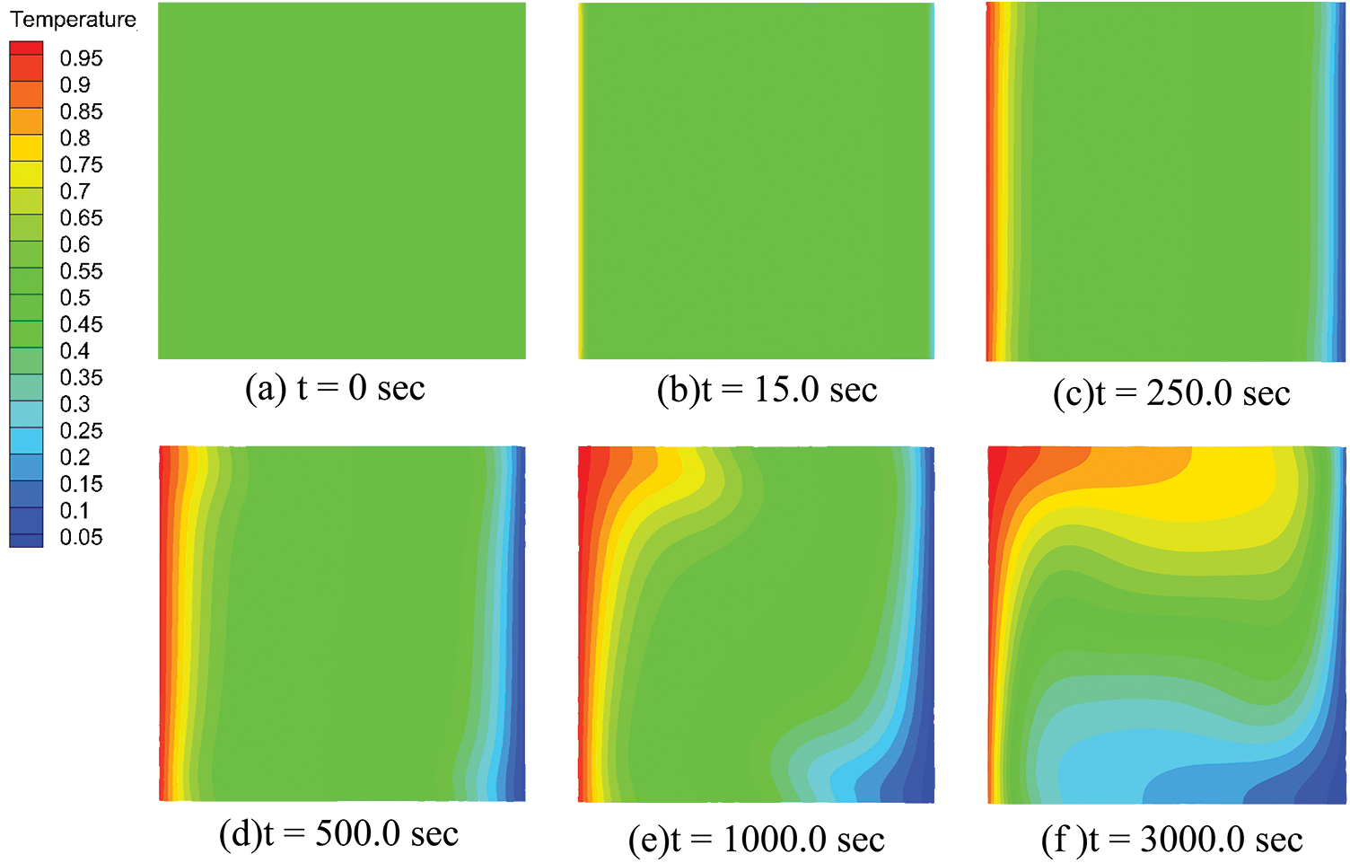
Figure 4: Temperature distribution using ULPH method from initial to steady state for Ra = 105

Fig. 5 shows the temperature (T*), horizontal velocity (Vx), and vertical velocity (Vy) for the steady state at different Rayleigh numbers (Ra = 103, Ra = 104, and Ra = 105). The temperature distribution of particles becomes widespread with the increase in Rayleigh numbers. As shown in Fig. 5a1, for Ra = 103, heat transfer is mainly carried out through conduction, and the influence of convection is relatively weak. The vortex motion generated by natural convection is also not significant. As the Rayleigh number increases to Ra = 104, shown in Fig. 5a2 and Ra = 105, shown in Fig. 5a3, the influence of convection becomes more significant, and the vortex motion caused by natural convection becomes stronger. This phenomenon can be explained as follows. As the Rayleigh number increases, the buoyancy of the fluid rises, leading to more intense fluid motion. Meanwhile, the thinning of the thermal boundary layer indicates that natural convection dominates heat transfer with the increase of Rayleigh number. From the velocity components shown in Fig. 5b,c, it can be seen that as Ra increases, the distribution of horizontal velocity (Vx) becomes more concentrated, and the vertical velocity (Vy) moves toward the sidewall, resulting in a significant thinning of the boundary layer. It further indicates that natural convection strengthens with the increase in Rayleigh number.

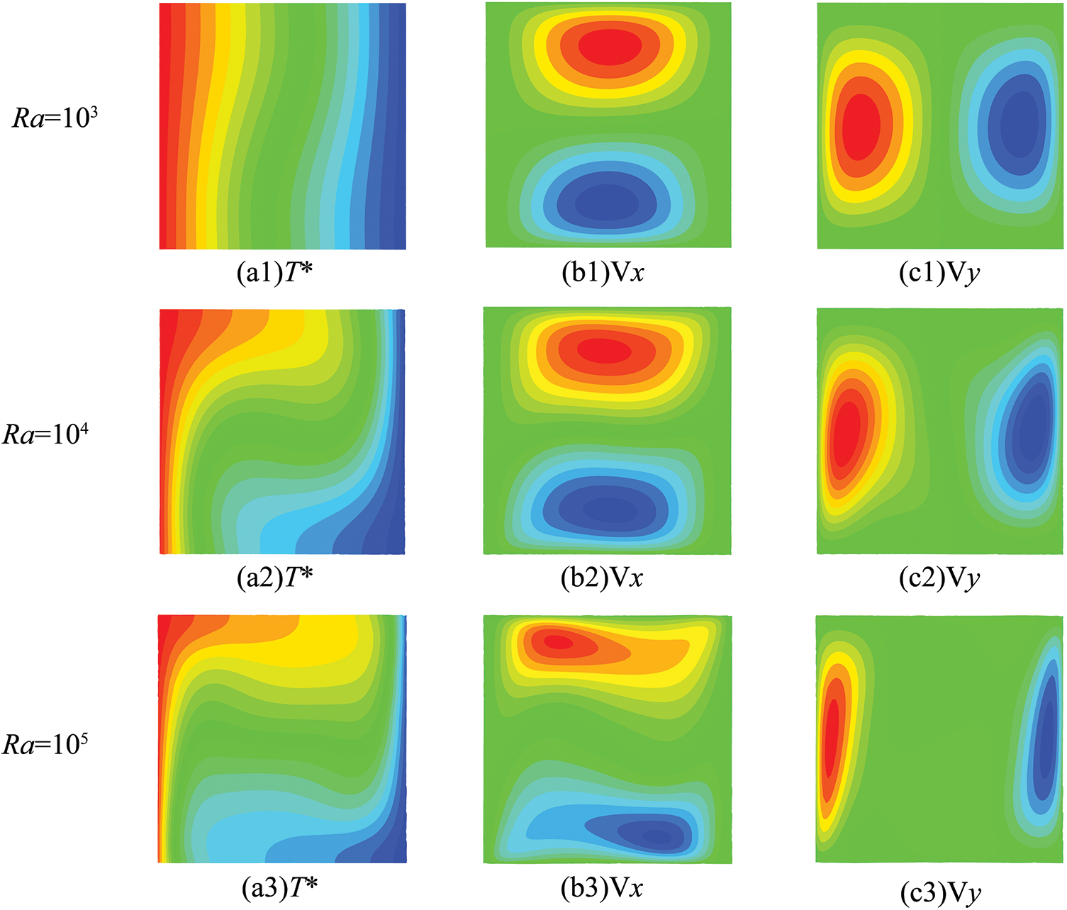
Figure 5: The distributions of temperature and velocity components (Vx and Vy) at the steady state under different Rayleigh numbers. (a) Temperature, (b) horizontal velocity component, and (c) velocity component

To quantitatively verify the accuracy of ULPH results, Fig. 6 presents the velocity components (Vx, Vy) along the central axis and the Nusselt number (Nu) along the cold wall (X = 1.0) for different Ra. Fig. 6a shows the steady-state horizontal velocity (Vx) along the horizontal axis (X = 0.5). Similarly, Fig. 6b presents the vertical velocity (Vy) distribution along the vertical axis (Y = 0.5). It can be seen that the velocity component curves are symmetrically distributed, and the changes in velocities increase significantly as Ra rises, while particles near the center position remained slowly. The velocity components show a good agreement by comparing the results of Wan et al. [8] using the discrete singular convolution (DSC) method. To further demonstrate the capability of ULPH method in simulating natural convection, we calculated the Nusselt number distribution along the cold wall. The expression of the Nusselt number is as follows:

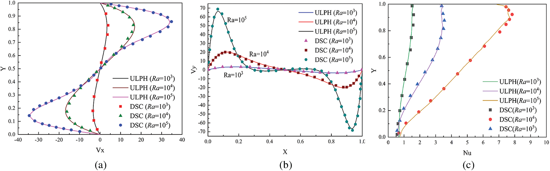
Figure 6: The steady-state velocity component along the central axis at various Rayleigh numbers compared with the results of Wan et al. [8] using the DSC method. (a) Vx at X = 0.5, (b) Vy at Y = 0.5, and (c) Nusselt number distribution along the cold wall

Nu|wall =LTH−TC|∂T∂x|wall .(31)

As depicted in Fig. 6c, the Nusselt distribution calculated using the ULPH method matches the DSC results well. We also observed a slight difference near Y = 1.0, which could be attributed to the non-uniform distribution of particles in the corner.

Fig. 7 shows the steady-state temperature curves along the central axis (Y = 0.5) at different Rayleigh numbers (Ra). The temperature distribution is typically linear at Ra = 103. As Ra increases, the temperature distribution no longer possesses a linear pattern. The curvature of the temperature curve increases across both ends of the axis with the increase in the Ra. It is consistent with the temperature distribution contour plot in Fig. 5. These findings closely align with FEM results by Aly [11].

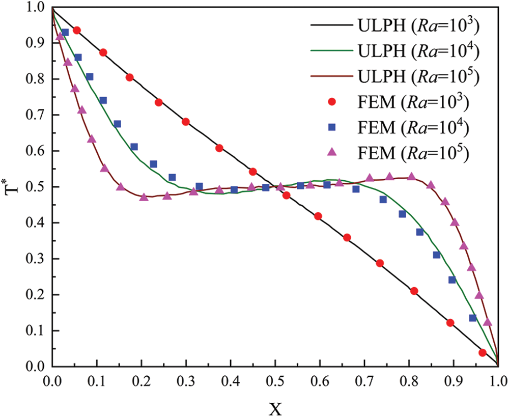
Figure 7: The steady-state temperature profiles along the central axis (Y = 0.5) at various Rayleigh numbers compared with Aly’s results [11] using the FEM method

3.3 Square Cavity with Localized Heating from Below

This section presents natural convective heat transfer simulations in square enclosures heated from below. The square cavity length (H) was determined to be 0.04 m (see Fig. 8). The left and right vertical walls were maintained at a low temperature of Tc = 300 K. The bottom boundary had a constant temperature heating zone (L < H), with a heating temperature Th. We chose a coefficient ε = L/H to represent the range of local heating. The rest of the bottom boundary and the entire top boundary were set to be adiabatic. The fluid parameters in this case were as follows. Initial density ρ0 = 1.0 kg/m3, viscosity coefficient μ = 2.0 × 10−5 Pa⋅s, thermal conductivity k = 0.02816 W/(m⋅K), specific heat capacity Cp = 1065 J/(kg⋅K), and the thermal expansion coefficient β = 0.003 K−1. The initial temperature of fluid T0 = Tc. The gravitational acceleration was taken as g = 10 m/s2 in the negative direction along the y-axis. Moreover, the value Pr = 0.71 was calculated by Eq. (30). Similarly, Ra = ρ02Cpgβ(Th – Tc)H3/(kμ) = 3408(Th – Tc) was controlled by Th. We calculated the natural convection results for Ra = 103, 104, and 105, corresponding to Th = 300.29343 K, 302.9343 K, and 329.343 K, respectively.

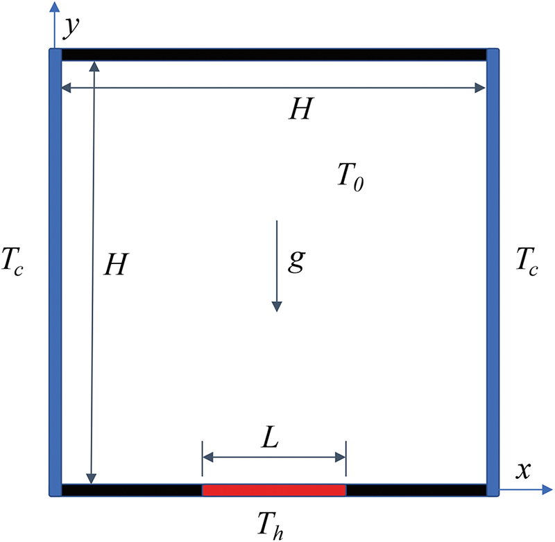
Figure 8: Schematic diagram for natural convection in a cavity with localized heating from below

The results of steady-state temperature distribution for different Rayleigh numbers (Ra = 103, Ra = 104, and Ra = 105) and different heating zone (ε = 0.2 and ε = 0.8) are shown in Fig. 9. It can be seen that the extent of the heating zone has a significant impact on the final result. As ε increases, the distribution range of the steady-state fluid temperature field expands. A significant temperature gradient distribution is observed near the bottom adiabatic boundary. At Ra = 103, as shown in Fig. 9a1,c1, heat transfer was primarily through conduction, and the effect of convection was not significant. However, at Ra = 105, as shown in Fig. 9a3,c3, distinct convective phenomena could be observed. Fluid particles near the bottom heating region experienced an increase in temperature due to the effect of heat conduction, leading to an upward buoyant force. As particles near the heating region moved upwards, particles in the cooler regions on both sides were carried along by the warmer particles, resulting in convective motion. Meanwhile, the number of particles in the warmer region decreased, reducing the pressure in this area. As a result, particles from both sides of the heating region continuously replenished the low-pressure area with high temperature, forming a vortical motion. This phenomenon was validated at Ra = 105, where the vortical motion of particles with low temperatures moving towards the warmer region near the bottom was observed.

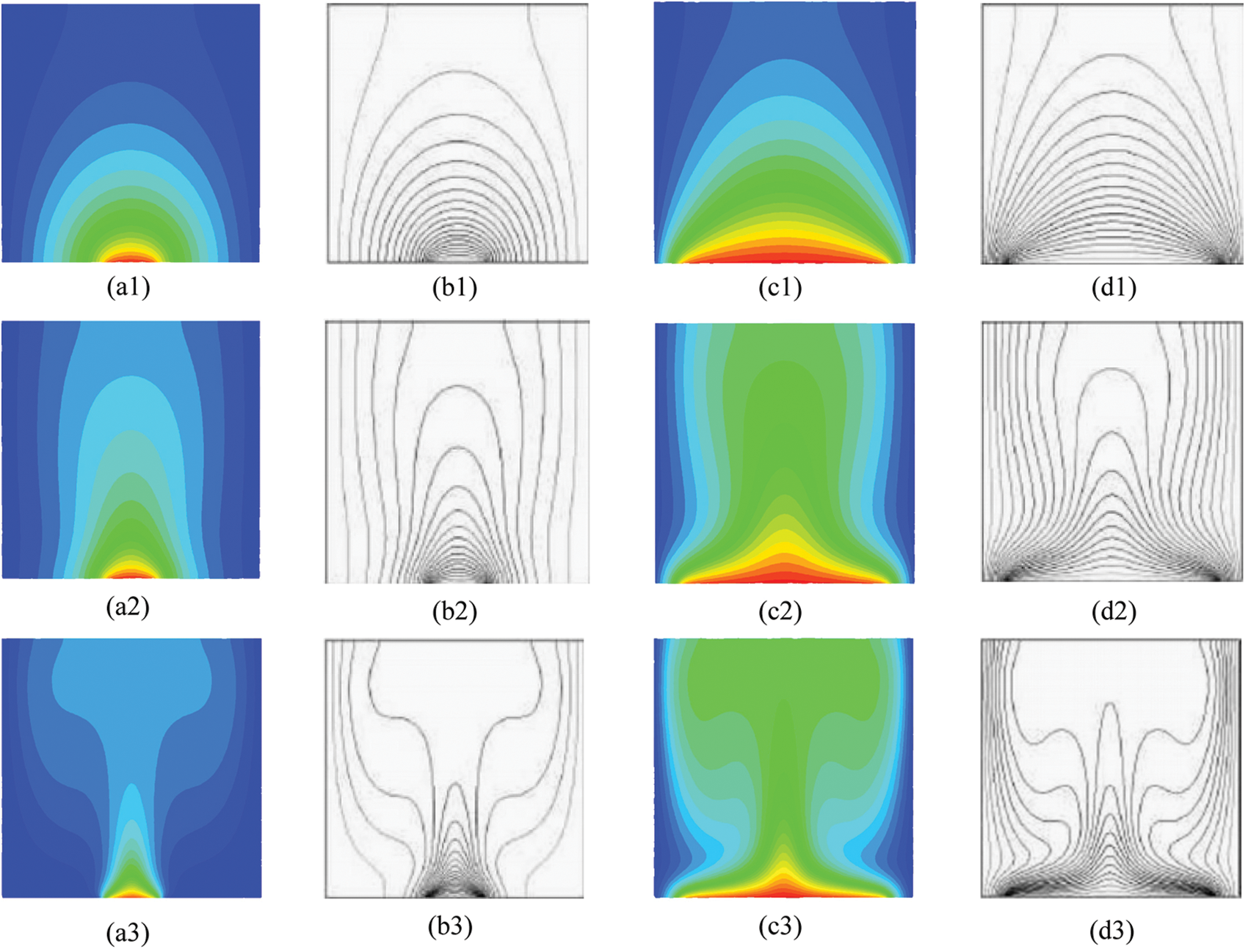
Figure 9: Steady-state temperature distribution against the numerical results by Calcagni et al. [25] under different Reynolds numbers (Top: Ra = 103, middle: Ra = 104, and bottom: Ra = 105). (a) ε = 0.2, by ULPH, (b) ε = 0.2, by FVM, (c) ε = 0.8, by ULPH, and (d) ε = 0.8, by FVM

The results obtained by ULPH simulation are consistent with the solutions using the finite volume method (FVM) by Calcagni et al. [25], further verifying the accuracy and reliability of the ULPH method.

To quantitatively validate the accuracy, we calculated the average Nusselt number for three heating zones with ε = 0.2, ε = 0.4, and ε = 0.8, in addition to Pr = 0.71, and Ra = 105. The expression for the average Nusselt number is given below:

Nuaverage=∫1−ε21+ε2Nu(X)⋅dX.(32)

Fig. 10 shows the distribution of the average Nusselt number over time. The average Nusselt number rapidly decreases initially and gradually reaches a steady state. After steady state, the numerical outcomes of average Nusselt numbers acquired from three heating zones closely match the numerical find ings using FVM by Calcagni et al. [25] as well as using the finite difference method (FDM) by Aydin et al. [26].

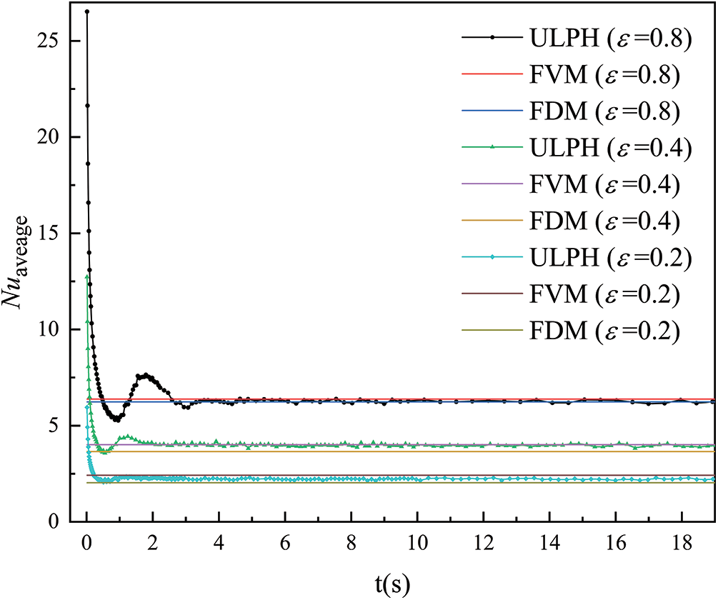
Figure 10: The average Nusselt number for different heating zones, compared with the numerical results using FVM [25] and FDM [26]

3.4 Natural Convection in Two Concentric Cylinders

The final benchmark test case involves natural convection in two concentric cylinders. Fig. 11 shows two concentric circles of different radii with R1 = D1/2 = 0.02 m and R2 = D2/2 = 0.052 m. The inner circle was designated as the heating boundary with a constant temperature Th = 323.664 K. Similarly, the outer circle served as the cold boundary, maintained at a constant temperature Tc = 300 K. The angle θ in Fig. 11 is used to describe the positions along different radii of the cylinders. The parameters of the fluid are as follows. The initial density ρ0 = 1.096 kg/m3, the viscosity coefficient μ = 2.0 × 10−5 Pa⋅s, the thermal conductivity k = 0.02816 W/(m⋅K), the specific heat capacity Cp = 1006.3 J/(kg⋅K), and the fluid thermal expansion coefficient β = 0.003 K−1. The initial temperature of the fluid inside the square cavity was T0 = Tc. The gravitational acceleration g = 10 m/s2 in the negative y-axis direction. The Rayleigh number, Ra = ρ02Cpgβ(Th - Tc)D13/(kμ), is 97600, which is consistent with the references [12,21].

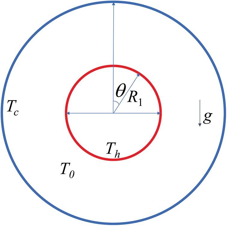
Figure 11: Schematic diagram for natural convection in two concentric cylinders

Fig. 12a–f shows the snapshots of the temperature distribution from the initial state to the steady state with particle spacing dx = 0.0005 m. The results clearly illustrate the natural convection of particles. At the heated wall boundary, fluid temperature increases due to heat conduction, leading to upward buoyancy and fluid motion. As the heated fluid rises and encounters the cold wall boundary, it spreads outward along the perimeter, generating pronounced vortex motion. Simultaneously, fluid near the inner perimeter moves upward from the bottom, forming natural convection within the circular enclosure. A distinct thermal boundary layer is visible at the inner boundary. In contrast, a significant low-temperature boundary layer appears at the outer boundary, indicating predominant heat conduction influence near the boundaries.

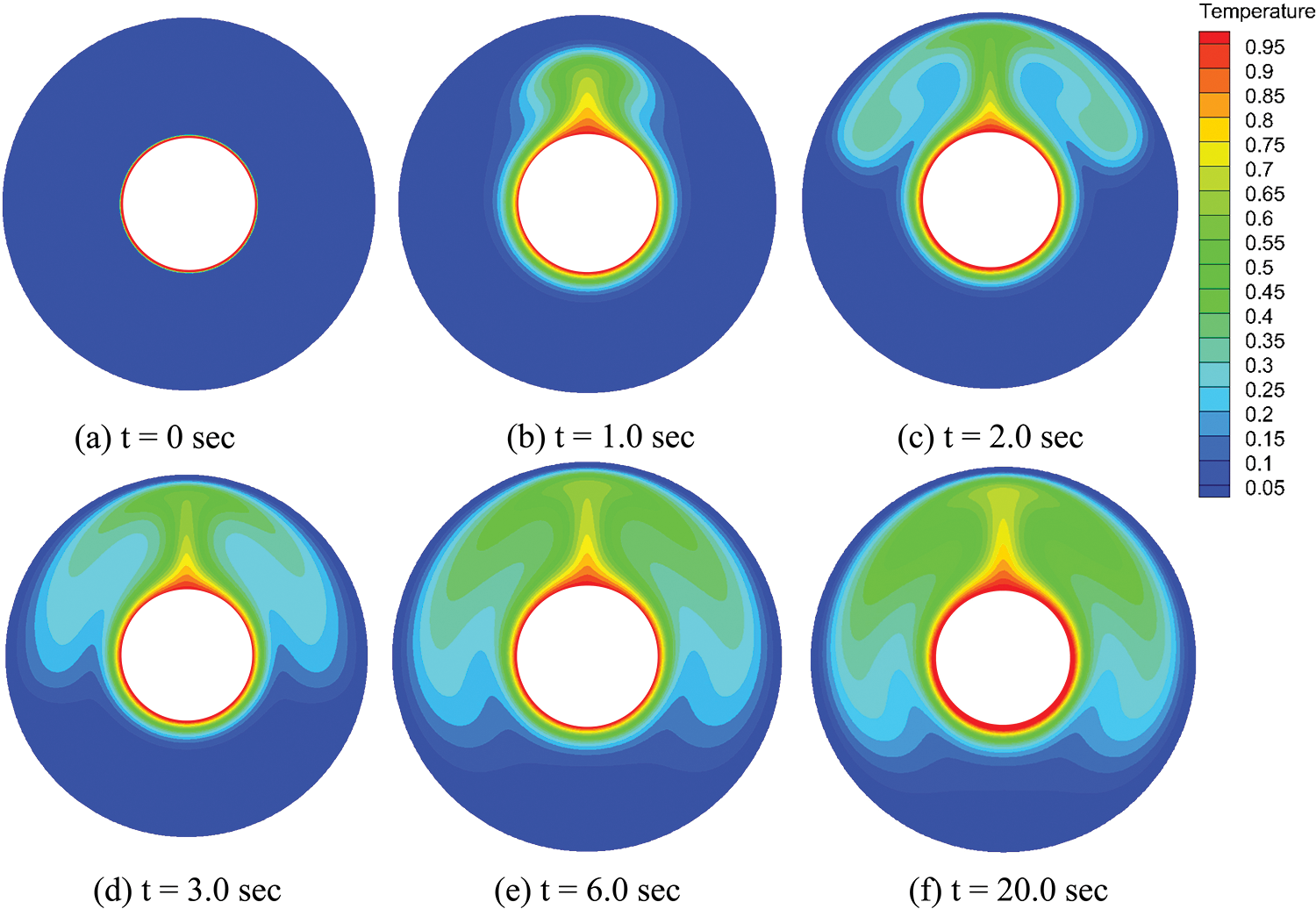
Figure 12: Snapshots of the temperature distribution from initial to steady states

Fig. 13a1–c1 shows the contour plots of temperature and velocity components within the circular enclosure at a steady state using the ULPH method. The temperature is represented using the dimensionless temperature (T*). Moreover, the velocities, u and v, denote the actual velocity components of the fluid. As shown in Fig. 13b1,c1, the heated air rises towards the upper region and splits into two streams. Subsequently, these streams propagate along the outer curved walls of the cavity, where they blend with the hot air surrounding the inner cylinder. The results obtained from the ULPH method are compared with numerical results obtained using the SPH method, as shown in Fig. 13a2–c2 [12]. The temperature and velocity results obtained from simulating natural convection in concentric circular enclosures using the ULPH method closely match those reported in the literature, highlighting the effectiveness of ULPH in solving natural convection problems.

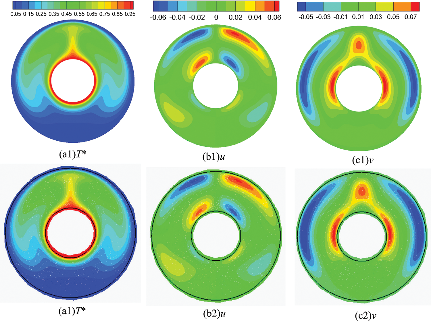
Figure 13: Steady-state results of dimensionless temperature (T*) and velocity components, u and v, in two concentric cylinders. Upper: ULPH method, lower: SPH method by Ng et al. [12]

For a quantitative comparison, Fig. 14 displays the dimensionless temperature distribution along the radial direction at the following angles. θ = 0°, 30°, 60°, 90°, 120°, and 150°. The results obtained from the ULPH method were compared with experimental data from Kuehn et al. [4] and other numerical solutions, such as FVM and SPH [12], and the unstructured moving particle pressure mesh (UMPPM) method [27], showing excellent agreement with these findings.

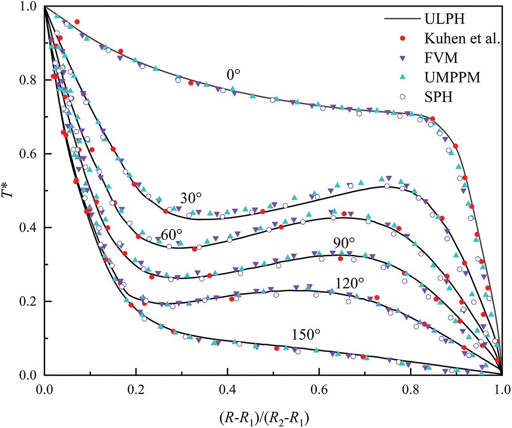
Figure 14: The radial distribution of dimensionless temperature (T*) at various angles: θ = 0°, 30°, 60°, 90°, 120°, and 150°

4  Conclusions

In this study, a second-order ULPH formulation of the non-isothermal buoyant flow model was explicitly devised to simulate natural convection. The Lagrangian forms of the momentum and energy equations were solved using second-order nonlocal differential operators to obtain the velocity and temperature variation rate. The numerical method was validated by comparing several benchmark cases, such as natural convection in a square cavity or between two concentric cylinders. The outcomes derived from the method outlined in this study exhibit notable consistency with findings documented in existing literature.

In future work, analysis of natural convection at high Rayleigh numbers will be conducted. As fluid motion becomes unstable and chaotic under these conditions, turbulence becomes a critical consideration. Therefore, turbulent models like large eddy simulation (LES) and direct numerical simulation (DNS) will be developed and investigated within the ULPH framework. Given the substantial number of particles required for turbulence calculations, utilizing graphics processing unit (GPU) parallel computing techniques within the ULPH framework will be essential for future advancements.

Acknowledgement: The authors are grateful to the editor and reviewers for improving this article.

Funding Statement: The authors would like to thank the support from the National Natural Science Foundations of China (Nos. 11972267 and 11802214), the Open Foundation of the Hubei Key Laboratory of Theory and Application of Advanced Materials Mechanics and the Open Foundation of Hubei Key Laboratory of Engineering Structural Analysis and Safety Assessment.

Author Contributions: The authors confirm contribution to the paper as follows: study conception and design: Junsong Xiong, Xin Lai; data collection: Junsong Xiong, Zhen Wang; analysis and interpretation of results: Junsong Xiong; draft manuscript preparation: Junsong Xiong; management and coordination: Xin Lai, Shaofan Li, Xiang Liu, Lisheng Liu. All authors reviewed the results and approved the final version of the manuscript.

Availability of Data and Materials: The data and related programs are available from the first and corresponding authors upon reasonable request.

Conflicts of Interest: The authors declare that they have no conflicts of interest to report regarding the present study.

References

1. Khanafer K, Vafai K, Lightstone M. Buoyancy-driven heat transfer enhancement in a two-dimensional enclosure utilizing nanofluids. Int J Heat Mass Transf. 2003;46(19):3639–53. doi:10.1016/S0017-9310(03)00156-X. [Google Scholar] [CrossRef]

2. Hatami M, Song D, Jing D. Optimization of a circular-wavy cavity filled by nanofluid under the natural convection heat transfer condition. Int J Heat Mass Transf. 2016;98:758–67. doi:10.1016/j.ijheatmasstransfer.2016.03.063. [Google Scholar] [CrossRef]

3. Liang YY, Sun ZG, Xi G, Liu L. Numerical models for heat conduction and natural convection with symmetry boundary condition based on particle method. Int J Heat Mass Transf. 2015;88:433–44. doi:10.1016/j.ijheatmasstransfer.2015.04.105. [Google Scholar] [CrossRef]

4. Kuehn TH, Goldstein RJ. An experimental and theoretical study of natural convection in the annulus between horizontal concentric cylinders. J Fluid Mech. 1976;74(4):695–719. doi:10.1017/S0022112076002012. [Google Scholar] [CrossRef]

5. Sheikholeslami M, Gorji-Bandpy M, Ganji DD. Numerical investigation of MHD effects on Al2O3-water nanofluid flow and heat transfer in a semi-annulus enclosure using LBM. Energy. 2013;60:501–10. doi:10.1016/j.energy.2013.07.070. [Google Scholar] [CrossRef]

6. Yang XF, Kong SC. Numerical study of natural convection in a horizontal concentric annulus using smoothed particle hydrodynamics. Eng Anal Bound Elem. 2019;102:11–20. [Google Scholar]

7. Davis GDV. Natural convection of air in a square cavity: a bench mark numerical solution. Int J Numer Methods Fluids. 1982;3(3):249–64. [Google Scholar]

8. Wan DC, Patnaik BSV, Wei GW. A new benchmark quality solution for the buoyancy-driven cavity by discrete singular convolution. Numer Heat Transf, Part B: Fundam. 2001;40(3):199–228. [Google Scholar]

9. Chaniotis AK, Poulikakos D, Koumoutsakos P. Remeshed smoothed particle hydrodynamics for the simulation of viscous and heat conducting flows. J Comput Phys. 2002;182(1):67–90. [Google Scholar]

10. Szewc K, Pozorski J, Tanire A. Modeling of natural convection with smoothed particle hydrodynamics: non-boussinesq formulation. Int J Heat Mass Transf. 2011;54(23–24):4807–16. [Google Scholar]

11. Aly AM. Modeling of multi-phase flows and natural convection in a square cavity using an incompressible smoothed particle hydrodynamics. Int J Numer Methods Heat Fluid Flow. 2015;25(3):513–33. [Google Scholar]

12. Ng KC, Ng YL, Sheu TWH, Alexiadis A. Assessment of smoothed particle hydrodynamics (SPH) models for predicting wall heat transfer rate at complex boundary. Eng Anal Bound Elem. 2020;111:195–205. [Google Scholar]

13. Yang PY, Huang C, Zhang ZL, Long T, Liu MB. Simulating natural convection with high Rayleigh numbers using the smoothed particle hydrodynamics method. Int J Heat Mass Transf. 2021;166(2):120758. doi:10.1016/j.ijheatmasstransfer.2020.120758. [Google Scholar] [CrossRef]

14. Li GY, Ma XJ, Zhang BW, Xu HW. An integrated smoothed particle hydrodynamics method for numerical simulation of the droplet impacting with heat transfer. Eng Anal Bound Elem. 2021;124:1–13. doi:10.1016/j.enganabound.2020.12.003. [Google Scholar] [CrossRef]

15. Tu QS, Li SF. An updated Lagrangian particle hydrodynamics (ULPH) for Newtonian fluids. J Comput Phys. 2017;348:493–513. doi:10.1016/j.jcp.2017.07.031. [Google Scholar] [CrossRef]

16. Yao WW, Zhou XP, Qian QH. From statistical mechanics to nonlocal theory. Acta Mech. 2022;233(3):869–87. doi:10.1007/s00707-021-03123-0. [Google Scholar] [CrossRef]

17. Yin P, Zhou XP. Updated Lagrangian nonlocal general particle dynamics for large deformation problems. Comput Geotech. 2024;166:106019. doi:10.1016/j.compgeo.2023.106019. [Google Scholar] [CrossRef]

18. Lai X, Li SF, Yan JL, Liu LS, Zhang AM. Multiphase large-eddy simulations of human cough jet development and expiratory droplet dispersion. J Fluid Mech. 2022;942:A12. doi:10.1017/jfm.2022.334. [Google Scholar] [CrossRef]

19. Yan JL, Li SF, Kan XY, Zhang AM, Lai X. Higher-order nonlocal theory of updated lagrangian particle hydrodynamics (ULPH) and simulations of multiphase flows. Comput Methods Appl Mech Eng. 2020;368(1):1–28. doi:10.1016/j.cma.2020.113176. [Google Scholar] [CrossRef]

20. Monaghan JJ. Simulating free surface flows with SPH. J Comput Phys. 1994;110(2):399–406. doi:10.1006/jcph.1994.1034. [Google Scholar] [CrossRef]

21. He F, Chen YX, Wang LQ, Li SZ, Huang C. A multi-layer SPH method to simulate water-soil coupling interaction-based on a new wall boundary model. Eng Anal Bound Elem. 2024;164:105755. doi:10.1016/j.enganabound.2024.105755. [Google Scholar] [CrossRef]

22. Morris JP, Fox PJ, Zhou Y. Modeling low Reynolds number incompressible flows with curved boundaries using SPH. J Comput Phys. 1997;136(1):214–26. doi:10.1006/jcph.1997.5776. [Google Scholar] [CrossRef]

23. Adami S, Hu XY, Adams NA. A generalized wall boundary condition for smoothed particle hydrodynamics. J Comput Phys. 2012;231(21):7057–75. doi:10.1016/j.jcp.2012.05.005. [Google Scholar] [CrossRef]

24. Chai T, Draxler RR. Root mean square error (RMSE) or mean absolute error (MAE)?—Arguments against avoiding RMSE in the literature. Geosci Model Dev. 2014;7(3):1247–50. doi:10.5194/gmd-7-1247-2014. [Google Scholar] [CrossRef]

25. Calcagni B, Marsili F, Paroncini M. Natural convective heat transfer in square enclosures heated from below. Appl Therm Eng. 2005;25(16):2522–31. doi:10.1016/j.applthermaleng.2004.11.032. [Google Scholar] [CrossRef]

26. Aydin O, Yang WJ. Natural convection in enclosures with localized heating from below and symmetrical cooling from sides. Int J Numer Methods Heat Fluid Flow. 2000;10(5):518–29. doi:10.1108/09615530010338196. [Google Scholar] [CrossRef]

27. Ng KC, Sheu TWH, Hwang YH. Unstructured moving particle pressure mesh (UMPPM) method for incompressible isothermal and non-isothermal flow computation. Comput Methods Appl Mech Eng. 2016;305:703–38. doi:10.1016/j.cma.2016.03.015. [Google Scholar] [CrossRef]