An Updated Lagrangian Particle Hydrodynamics (ULPH)-NOSBPD Coupling Approach for Modeling Fluid-Structure Interaction Problem

Nomenclature

1  Introduction

Ship and ocean engineering is being vigorously developed due to the strategic needs of maritime power; the related fields of structural mechanics and hydrodynamics have yielded fruitful results [1,2]. Typical high-speed hydrodynamic problems such as the high-speed motion of vehicles in the water, underwater explosion, and structural damage [3] involve complex processes such as transient strong impact load, large movement of structures, bubble growth, and collapse. These problems are closely related to the comprehensive performance of modern ships and their weapons and equipment. However, these are multi-physical field problems involving interaction between moving or deformed structures and surrounding or internal fluids. In other words, the above-mentioned problems can be characterized as typical multiphase fluid-solid coupling and vapor-solid-liquid three-phase coupling problems [4].

Since fluid-structure interaction problems are complex and involve many nonlinear factors, obtaining analytical solutions through theoretical derivation is often difficult. Numerical simulation and model tests have become two common ways to analyze fluid-structure interaction problems. The time cost of test data and the cost of trial and error are high for model tests. In contrast, numerical simulation has the advantages of low cost, short cycle, and clear physical process, playing an increasingly important role in ship and ocean engineering.

In recent years, many numerical calculation methods have emerged with the development of computer technology. Currently, based on different discretization and solution forms, numerical simulation methods can be classified into grid methods described by Euler, such as volume-of-fluid (VOF) [5,6], level set method (LS) [7,8], lattice Boltzmann method (LBM) [9,10], and forward tracking method [11,12]. Furthermore, Lagrangian descriptions of meshless methods are also often used, such as Smooth Particle Hydrodynamics (SPH) [13], reproducing kernel particle method (RKPM) [14], moving particle semi-implicit (MPS) [15], and material point method (MPM) [16]. More recently, the Updated Lagrangian Particle Hydrodynamics (ULPH) originally proposed by Tu et al. [17] is also often used. The mesh method suffers from mesh distortion when solving the fluid-structure coupling problem with large deformation. The latter meshless method benefits from the natural Lagrangian characteristics and gradually completes particle approximation theory advantages. Moreover, it is not limited by boundary deformation when simulating large deformation problems [18]. Therefore, it has been widely used in fluid-structure interaction problems.

ULPH is another meshless particle method successfully implemented to solve fluid dynamics problems. Inspired by peridynamics [19], RKPM [14], and SPH, the local differential operator in the Navier-Stokes equations is replaced by a non-local differential operator (NDO). Since the non-local continuous function space contains a function space much larger than the local continuous function space, it may capture more physical content than the local continuum CFD method. Compared with the classical SPH method, ULPH eliminates the tensile instability and the accuracy loss caused by the kernel approximation. Therefore, ULPH is suitable for describing fluid motion in more complex flow fields. ULPH employs the updated Lagrangian formulation and selects the current configuration as the updated reference configuration instead of using the initial configuration as the reference configuration. Furthermore, ULPH continuously updates the reference configuration during calculation. The total Lagrangian method defined and described in the initial configuration can be used instead of using the variables as SPH and molecular dynamics (even the initial configuration can be chosen as the reference configuration). As pointed out in [20], using the updated configuration as a reference configuration is advantageous as another rapidly developing meshless method. The basic idea of peridynamics (PD), proposed by Silling [21], is a non-local continuous theory that uses non-local integral equations. A discontinuous displacement field can be naturally included in the governing equations. Hence, it has natural advantages in simulating crack initiation and propagation in materials, becoming a research hotspot. There are three different branches in peridynamic theory: bond-based peridynamics (BB-PD) [21], state-based peridynamics (SB-PD) [22] and non-ordinary state-based peridynamics (NOSB-PD) [23]. Zhou et al. [24] proposed a new fully coupled hydrodynamic model of bond-based peridynamics to simulate the pressured and fluid-driven fracturing processes in fractured porous rocks. A complete discretization model and numerical integration algorithm for the ULPH and BB-PD coupling formulas have been successfully established [25]. These methods were used to simulate ice-water interaction under impact load, i.e., ice fragmentation and fracture. Yan et al. [26] developed a set of high-order non-local differential operators in the ULPH framework and applied them to solve multiphase flow problems [27]. The results show that the ULPH method is more accurate than SPH in modeling and simulating multiphase flow problems.

Despite the success in the problem of coupling BB-PD with ULPH, the interaction between two material points in the bond-based peridynamics depends only on the deformation of the bond between that material point. This assumption restricts the Poisson ratio of the solid model. Therefore, solving typical FSI-based problems by coupling PD with ULPH is still difficult. Since ULPH-NOSBPD has a good potential for structural analysis, combining their advantages is an important research topic. This work is motivated to develop a ULPH-NOSBPD method that simultaneously handles complex fluid flows, large structural deformations, and even failures.

2  Numerical Approach

2.1 Update Lagrangian Particle Hydrodynamics for Newtonian Fluids

2.1.1 Governing Equations

In this paper, the fluid is assumed to be weakly compressible without considering thermal effects. Energy changes have a minor influence on the fluid characteristics when the pressure peak of the weakly compressible fluid is below 1 GPa. Thus, the fluid is considered to be isentropic. The fluid dynamics formulation can be solved using the Navier-Stokes equations. The Navier-Stokes equations can describe the relationship between a fluid’s velocity, pressure, density, and temperature. The Navier-Stokes equations are a set of coupled differential equations that can theoretically be solved using calculus methods for a given flow problem.

In the Lagrangian form, the governing equations for the isentropic flow comprise mass and momentum conservation laws. The general form of the governing equations [28] is written as follows:

DρDt=−ρ∇⋅v(1)

DvDt=1ρ∇⋅σ+g(2)

where D/Dt represents the material time derivative, v represents the velocity vector, ρ is the fluid density, g is the gravity acceleration (9.81 m/s2 is used in the present paper), and σ represents the Cauchy stress tensor [26], i.e., the summation of a pressure term −pI (hydrostatic stress or volumetric stress) and a viscosity term (deviatoric stress):

σ=−pI+τ(3)

where I is the unit second-order tensor. The viscous stress τ is expressed as follows:

τ=2με˙(4)

where μ is the dynamic viscosity and ε˙ is the rate of shear strain tensor as follows:

ε˙=12[∇⊗v+(∇⊗v)T]−13(∇⋅v)I(5)

The above Navier-Stokes equations are non-closed at this stage. Additional state equations must be added to establish the connection between pressure p and density ρ. The Tait equation [29] can be connected to solve the Navier-Stokes equations for the weakly compressible fluid. In the paper, the evolution of the pressure from the density is determined by following a linearized form of the Tait equation as the equation of state, as follows:

p=c02ρ0γ[(ρρ0)γ−1](6)

where ρ0 is the density in the reference configuration and γ is the characteristic index coefficient (equal to 7 for water). Parameter c0 is the reference sound speed to control the compressibility of the fluid, which should satisfy the density variation of less than 1%. To satisfy the weakly compressible properties, it is necessary to use the reference sound speed [27] as follows:

c0≥10max(pmax/ρ0,Umax)(7)

where the maximum expected pressure and velocity in the computational domain are represented by pmax and Umax. The true sound speed in the fluid is not used to increase the time step size and improve the computational efficiency.

2.1.2 Optimal Non-Local Differential Operators

Calculating gradient and divergence in the flow field is a key part of computational fluid dynamics because the continuity equation is solved through the divergence of the velocities. However, the momentum equation is solved by the stress divergence and the velocity gradient. Eqs. (1)–(3) are the governing equations in local form. The grid-like numerical methods divide the entire computational domain into grids and apply local theory ideas to solve the governing equations numerically. For the meshless method, it is necessary to discretize the entire computational domain into particles. Each particle has the properties of density, mass, pressure, and velocity. Then, the governing equations are discretized using the idea of non-local theory.

In the ULPH framework [17], the non-local differential operator is used instead of the local operator to calculate divergence, gradient, and curl:

∇I⋅(•):=∫ℋIω(xIJ)(Δ(•))⋅(MI−1xIJ)dVJ,(8)

∇I⊗(•):=∫ℋIω(xIJ)(Δ(•))⊗(MI−1xIJ)dVJ,(9)

∇I×(•):=∫ℋIω(xIJ)(MI−1xIJ)×(Δ(•))dVJ(10)

where operators (∇⋅(•)), (∇⊗(•)), and (∇×(•)) represent the non-local divergence, gradient, and curl operators, respectively; ℋI represents the support domain of particle I, as shown in Fig. 1, subscript J denotes the family member of particle I, and xIJ=xJ−xI. The symbol (•) represents the arbitrary field and Δ(•):=(•)J−(•)I is the finite difference operator. The function ω(xIJ) is the kernel function that must meet specific criteria (this function will be discussed later). Lastly, M is the shape tensor defined in the current configuration or the updated configuration [17]:

MI:=∫ℋIω(xIJ)xIJ⊗xIJdVJ(11)

Figure 1: Non-local theoretical models

The computational domain of ULPH is discretized as a sequence of particles with physical properties. The above non-local differential operator can be discretely rewritten as:

∇I⋅(•)=∑J=1Nω(xIJ)(Δ(•))⋅(MI−1xIJ)VJ(12)

∇I⊗(•)=∑J=1Nω(xIJ)(Δ(•))⊗(MI−1xIJ)VJ(13)

∇I×(•)=∑J=1Nω(xIJ)(MI−1xIJ)×(Δ(•))VJ(14)

The discretized form of the shape tensor Eq. (11) is reformulated as:

MI=∑J=1Nω(xIJ)xIJ⊗xIJVJ.(15)

2.1.3 DiscreteForm of Governing Equations

In ULPH, the current configuration Ωn at the time t = tn is chosen as the reference configuration, as described in [17,26], as shown in Fig. 1. The referential configuration is continuously updated as the computation proceeds. Therefore, the governing equations below are calculated under the current configuration.

Based on the above non-local differential operators and peridynamic theory [19], the continuous equation can be obtained in the non-local discrete form in the ULPH framework by substituting the non-local divergence operators Eq. (12) into the continuous equation Eq. (1):

DρIDt=−ρI∑J=1Nω(xIJ)(vJ−vI)MI−1xIJVJ,(16)

where VJ is the volume of the fluid particle, VJ=mJ/ρJ, m is the mass of the fluid particle, and ω(xIJ) is the kernel function. Selecting the kernel function is related to the numerical simulation’s accuracy, efficiency, and stability. In this paper, the Gaussian kernel function [30] is adopted to all simulations as the influence function ω and is defined as:

ω(r,h)=αd(e−(r/h)2−C)r≤δ,(17)

where r is the distance between two neighboring particles I and J, h is the smoothing length typically set to h=1.2Δx (Δx is the initial spacing of the particles), δ(δ=3h) is the size of the support domain of the particle, d is the spatial dimension, C is generally set to e−9, and the normalized coefficient αd is a coefficient associated to spatial dimension and the smoothing length:

αd=1hdπd/2(1−10e−9).(18)

According to the state-based peridynamic theory, the non-local form of the momentum equation [22] can be defined as:

ρIDvIDt=∫ℋI(TI(xIJ)−TJ(xJI))dVJ+b,(19)

where TI(xIJ) and TJ(xJI) denote the force state vector acting on particles I and J, and b is the external body force:

TI(xIJ)=ω(xIJ)σIMI−1xIJ,(20)

TJ(xJI)=ω(xJI)σJMJ−1xJI.(21)

Since ω(xIJ) = ω(xJI) and xJI=−xIJ, Eqs. (20) and (21) are substituted into Eq. (19). The momentum equation can be written as [31]:

ρIDvIDt=∫ℋIω(xIJ)(σIMI−1+σJMJ−1)xIJdVJ+b.(22)

The discrete form of the momentum equation is given by:

ρIDvIDt=∑J=1Nω(xIJ)(σIMI−1+σJMJ−1)xIJVJ+b.(23)

The symmetry between the particles can be guaranteed using the σIMI−1+σJMJ−1form in the momentum equation. Hence, the conservation of linear momentum and the conservation of angular momentum are guaranteed.

In the Cauchy stress tensor expression defined by Eq. (2), the pressure p can be calculated through the Tait equation of state in Eq. (6). According to the Tait equation of state, the density determines the pressure of the fluid. Therefore, a small change in density will cause a large pressure oscillation. For the fluid-structure interaction problems, pressure instabilities and density oscillations may occur in the fluid particle duration simulation. The density filter algorithm [32] is adopted to avoid this issue and obtain a stable and smooth pressure field, as follows:

ρInew =∑Jω(xIJ)mJ∑Jω(xIJ)VJ,(24)

where ρInew  is the corrected density. Moreover, the corrections are performed every twenty steps to reduce computation costs and avoid artificial diffusions.

The rate of shear strain tensor ε˙ in the proposed ULPH method can be written in a discrete form:

ε˙I=((∑J=1Nω(xIJ)mJρJvIJ⊗xIJ)MI−1)sym−13(∑J=1Nω(xIJ)mJρJvIJ⋅(MJ−1xIJ))I.(25)

An artificial viscosity term can be added to the right-hand side of the equation of motion to reduce unphysical or numerical oscillations and enhance stability when simulating impact/penetration problems. In this work, the Monaghan [13] type artificial viscosity function is used in the computation. It is modified in [31] to obtain the artificial viscosity formula in the ULPH framework as follows:

ΠI=αhc0ρ0∑J=1Nω(xIJ)πIJMI−1xIJVJ,(26)

where α is the coefficient of the artificial viscosity term that ranges from 0 to 0.5 depending on the problem, the term πIJ is expressed as follows:

πIJ={vIJ⋅xIJ|xIJ|2+(0.1h)2,vIJ⋅xIJ<00, otherwise .(27)

Therefore, the discretized motion governing the equation of ULPH after applying artificial viscosity can be rewritten as follows:

ρIDvIDt=∑J=1Nω(xIJ)(σIMI−1+σJMJ−1)xIJVJ+ΠI+b.(28)

2.2 Basic Concepts and Formulations of Non-Ordinary State-Based Peridynamics

In peridynamic theory, the research object in the spatial domain R is discretized into a series of peridynamic particles containing all physical information, such as position, velocity, and density. For every particle XJ(J=1,2,3,…,nI) there is a neighborhood of radius δ in space. The horizon is denoted as ℋx, as shown in Fig. 2. The particle interacts with every particle XJ(J=1,2,3,…,nI) in its neighborhood, u is the displacement vector of the particle, ξIJ is the relative position, i.e., ξIJ=XJ−XI, and the relative displacement is denoted by ηIJ, where ηIJ=u[xJ,t]−u[xI,t], as illustrated in Fig. 2.

Figure 2: Schematic diagram of the non-ordinary state-based peridynamics theory

In continuum mechanics, the equations of motion of a continuum with general dynamic motion are [33]:

ρ0u..=∇X⋅PT+ρ0b,(29)

where ρ0 is the current material density, u.. is the acceleration of material point, ∇X denotes the divergence of the first Piola-Kirchhoff stress P concerning the reference configuration, and b is the body force density. In peridynamics, the above balance equation of linear momentum is replaced by a non-local integral equation:

ρ0u..=L(x,t)+ρ0b.(30)

In the NOSB-PD theory [22], L(x, t) is a non-local integration of force density vector f (x, x′):

L=∫Vf(xA,xB)dVxB=∫ℋxI[TI(ξIJ,YI(ξIJ))−TJ(ξJI,YJ(ξJI))]dVXB,(31)

where TI(ξIJ,YI(ξIJ)) is the force vector state acted on material point XI due to material point XJ; the same principle applies TJ(ξJI,YJ(ξJI)). Then, the governing equations of motion are rewritten in the NOSB-PD form as:

ρ0u..=∫ℋxI[TI(ξIJ,YI(ξIJ))−TJ(ξJI,YJ(ξJI))]dVJ+ρ0b,(32)

where T is the force-vector state related to the stress of the first Piola-Kirchhoff; the unit of the force state is N/m6.

T_[xI,t]⟨ξIJ⟩=ω(ξIJ)PxIKxI−1⟨ξIJ⟩,(33)

where KxI−1 in Eq. (33) represents the inverse of the KxI and KxI is the shape tensor of the material point XI defined as:

KxI=∫ℋxIω(ξIJ)ξIJ⊗ξIJdVxJ,(34)

Parameter PxI in Eq. (33) is the first Piola-Kirchhoff stress tensor associated with the Cauchy stress tensor σ:

PxI=𝒥σxIFxI−T,(35)

where 𝒥=detFXI, and FXI is the non-local deformation gradient of the particle XI defined as follows:

FxI=∫ℋxI[ω(ξIJ)Y_⟨ξIJ⟩⊗ξIJ]dVxJKI−1.(36)

2.2.1 Constitutive Update under Finite Deformation

The zero-energy mode [34] in the NOSBPD model did have considerable significance to the computational stability and numerical accuracy. In our work, we have employed a kind of finite deformation algorithm which is proposed and used in previous work [35]. In the experience of our computations, this algorithm is capable of zero-energy control when used with the elastic model, Drucker-Prager constitutive model [35], with consideration of material fracture and failure.

Finite deformation happens during solid structure failure, and the Hughes–Winget algorithm [36] calculates Cauchy stress as a nonlinear formula when there is finite deformation. According to the continuum mechanics, by using displacement increment Δu, a material point can be transformed from its previous position in the current configuration of a solid body at time step n (xn) to its updated position at time step n + 1 (xn+1). Consider the one-parameter family of configurations at the time step n+α as follows:

xn+α=(1−α)xn+αΔu(37)

α takes the value 0.5 in this work. Eq. (36) is the peridynamics formulation of the first derivative of the position vector x under the reference configuration. According to the same derivation, the deformation gradient at the current configuration xn+α can be derived as:

Fn+α=∂xn+α∂X=(∑J∈HXIω(|ξ|)(xJ,n+α−xI,n+α)⊗ξ)⋅K−1(38)

Meanwhile, the gradient of displacement increment Δu with respect to the reference configuration can be written as:

C=∂(Δu)∂X=(∑J∈HXIω(|ξ|)(ΔuJ−ΔuI)⊗ξ)⋅K−1(39)

Therefore, the gradient of Δu at the configuration (xn+α) can be derived by the chain rule as:

G=(∂Δu)∂xn+α=C⋅Fn+α−1(40)

where G is the incremental deformation gradient, which can be written as the strain increment and the rotation increment:

γ=(G+GT)/2(41)

ω=(G−GT)/2(42)

Therefore, the effective stress increment can be calculated by the following equation:

Δσ=De:γ(43)

Finally, the constitutive update equation in the large deformation formula can be rewritten as follows:

σn+1=σ^n+Δσ(44)

σ^n=RT⋅σn⋅R(45)

R=I+(I−αω)−1⋅ω(46)

2.2.2 Failure Criterion

When the relative position between two particles meets certain conditions, their interaction will disappear forever, destroying the bond. A bond-breaking indicator μ [37,38] is introduced to describe the fracture of bonds:

μ(XI,t,ξ)={1s(t,ξ)<s00 otherwise ,(47)

where s0 is the extreme or critical stretch for a given bond, and s is the bond stretch defined as s=(|ξ+η|−|ξ|)/|ξ|:

s0=5G0/(9Kδx),(48)

where G0 represents energy release rate [39].

In peridynamics, enabling failure at the bond level is one of its advantages leading to unambiguous local damage φ at a material point XI defined as:

φ(XI,t)=1−∫HxIμ(XI,t,ξ)dVXJ∫HxIdVXJ.(49)

2.3 The Solid Boundary Conditions

When the ULPH method is used to numerically simulate problems related to fluid dynamics, there will be boundary types such as free surface, solid wall, and periodic boundaries. As shown in Fig. 3a, the support domain of fluid particles near the boundary will be truncated by the boundary, causing calculation errors and affecting the calculation accuracy. Therefore, investigating problems with boundaries requires special treatment at the boundaries.

Figure 3: The sketch of different solid boundary treatment methods

For the traditional particle method, there are three main effective methods for solid wall boundary processing: repulsive boundary method [13], mirror particle boundary [32], and fixed ghost boundary [40], as shown in Fig. 3b. Since the repulsive boundary method has only a single layer of boundary particles and does not address the problem of nuclear truncation, it may produce unphysical perturbations to the flow field pressure. The mirror particle boundary must dynamically generate virtual particles at each step, reducing the computational efficiency. Hence, the mirror particle boundary is only suitable for regular plane or right-angle boundaries. Moreover, it is difficult to determine the position of the mirrored virtual particle for complex boundaries. Hence, the fixed ghost boundary method is adopted in the current work.

The fixed ghost boundary method sets three to four layers of virtual boundary particles at the boundary to simulate wall conditions, which does not need to mirror the generated particles in each time step and complements the support domain of fluid particles to ensure that there is no kernel truncation problem. The physical variables of the fixed ghost boundary particles are interpolated from the neighboring fluid particles, thus ensuring effective interaction with the adjacent fluid particles. With the fixed ghost boundary method, various boundary conditions, including no-slip or free-slip boundary conditions, can be flexible-handled, leading to more accurate and stable fluid simulations [31,41]. The viscous force between ghost and fluid particles is trivial for the free-slip solid boundary condition. For the no-slip solid boundary condition, a virtual velocity vs is introduced to implement the interaction of the dummy particles of the fluid particles as follows:

vs=2vs⌢−v~I,(50)

where subscript S represents the ghost particle, vs⌢ represents the prescribed velocity of the solid ghost particle I, and v~I represents the interpolation from the neighboring fluid particles as [40]:

v~I=∑J=1NfvJω(xIJ)∑J=1Nfω(xIJ),(51)

where Nf refers to the number of neighborhood fluid particles within the horizon of a solid ghost particle I. The viscous force between solid wall particles and fluid particles can be obtained by substituting Eq. (50) into the viscous force calculation formula.

The pressure ps of the solid virtual particle can also be determined by interpolating its neighboring fluid particles. Moreover, the pressure of the solid wall particle can be regularized using the Shepard kernel [40]. Hence, the final calculation formula for the pressure of the solid wall particle can be obtained as follows:

ps=∑f=1Nfpfω(xsf)−(g−ai)⋅∑f=1Nfρfxsfω(xsf)∑f=1Nfω(xsf),(52)

Eq. (52) shows that only the fluid particles in the support domain are considered in the interpolation calculation of the solid wall particle pressure. In Eq. (52), ai is the acceleration of the solid wall boundary [25].

For the fixed solid wall boundary condition, the acceleration of the wall particle is set to ai = 0. Based on the pressure of the solid particle obtained by interpolation, the density of the solid particle can be evaluated by the equation of state [25]:

ρI=pIc02+ρ0.(53)

Subsequently, the mass of the solid particle can be obtained as:

mI=ρIV0,(54)

where V0 is the initial volume of a solid particle.

2.4 Time Integration Scheme

After discretization of the fluid-structure coupling model, additional solution strategies and updated algorithms are required to meet the accuracy and stability requirements during calculation and computer program implementation of the boundary conditions. This section focuses on the time integration method for explicit dynamical equations and the combined solution strategy for fluid and solid solvers.

Choosing the appropriate time integration method will also significantly affect the running efficiency of the program. The velocity and displacement of the solid particle for the solid part of PD calculated in this paper are updated by the Velocity-Verlet time integration method with given boundary conditions and initial conditions:

u.[xi,t+Δt2]=u.[xi,t]+Δt2×u..[xi,t]u(xi,t+Δt)=u(xi,t)+Δt×u.[xi,t+Δt2],u.[xi,t+Δt]=u.[xi,t+Δt2]+Δt2×u..[xi,t+Δt](55)

where Δt is the time step, u˙ and u are the velocity and displacement vectors, respectively. The size of the time step t should satisfy the CFL condition to maintain the stability and accuracy of the simulation [25].

In this study, the predictor-corrector method was used for the ULPH time integration of the fluid part (divided into two stages) due to the nature of the updated Lagrangian particle hydrodynamics algorithm:

In the prediction stepIn the correction step{ρIn+12=ρIn+Δt2(dρdt)nvIn+12=vIn+Δt2(dvdt)nxIn+12=xIn+Δt2vIn+12{ρIn+1=ρIn+Δt(dρdt)n+12vIn+1=vIn+Δt(dvdt)n+12.xIn+1=xIn+ΔtvIn+1(56)

3  NOSB-PD with ULPH Coupling Scheme

In this study, the partition decoupling solution method is used to solve the governing equations of the fluid-structure coupling system. The fluid and solid parts are solved separately by their solvers for the partition decoupling solution. Moreover, the data are exchanged through the coupling interface to meet the coupling conditions. The NOSB-PD theory is utilized in the solid region to describe the material behavior of solids due to its ease of handling damage or rupture processes. In contrast, the ULPH is used to model fluids. Therefore, a key step is dealing with the coupling interface in the computational domain of PD-ULPH to guarantee the transfer of force and deformation. Fig. 4 illustrates the PD-ULPH coupling scheme based on virtual particles.

Figure 4: Schematic illustration of the PD-ULPH coupling scheme

The force transfer mechanism from ULPH particles to PD particles is first considered. It is assumed there is a NOSB-PD particle A near the interface whose horizon contains a ULPH particle B. When the force state TA(ξ,Y(ξ)) of particle A is computed, the force state of the solid particle is calculated separately, ignoring the fluid particles in the immediate neighborhood. Only the forces of solid particles on solid particles in the support domain are considered.

There are usually two approaches to the force exerted by a fluid particle on a solid particle. A convenient approach is implementing the analysis from the continuum perspective. The forces exerted on solid bodies can be calculated by integrating the stresses along the solid (structures) surface (boundary) [42].

The other approach involves directly applying the pressure of the neighboring fluid particles in the support domain of the solid particle to the fluid particle, obtaining the force of the fluid acting on the solid. This approach is adopted here, where A represents the surface area of the solid particle.

FpB=∑B=1NfpBAAVAxAB|xAB|(57)

A similar situation to the one mentioned above occurs when a peridynamic particle A is located inside the support zone of a ULPH particle. When the interaction force acting on a ULPH particle is calculated and induced by a peridynamic particle, the peridynamic particle is considered a ULPH particle. As a result, this particle is involved in the equation’s computation of the shape tensor and the spatial velocity gradient tensor of the fluid particle. Therefore, the peridynamic particle participates in calculating every conservation law for that ULPH particle. For example, for the ULPH particle B, its linear momentum equation reads as:

ρBDvBDt=∑A=1Nω(xBA)(σBMB−1+σAMA−1)xBAVA+ΠB+b(58)

For a peridynamic particle A, which is treated as a ULPH particle, it is necessary to obtain its pressure and velocity v when using Eq. (3) to calculate σA. Its pressure is interpolated from the ULPH particle in the neighborhood to obtain Eq. (52). The density and mass are obtained via Eqs. (53) and (54), and the velocity is calculated from Eq. (50). Therefore, a fixed ghost boundary condition generates interaction between virtual particle A and fluid particle. Moreover, solid particles will provide fluid-solid boundaries for fluid particles. Lastly, the pressure interpolated on the solid will generate repulsive forces for fluid particles, preventing particles from penetrating each other.

It is worth mentioning that the shape tensor of the liquid will become an ill-conditioned matrix in this coupling method due to the influence of the solids in its neighborhood. A small disturbance will cause a large change in the inverse of the shape tensor when inverting the ill-conditioned shape tensor, affecting the calculation accuracy. Therefore, the fluid is calculated in the current configuration when calculating the shape tensor. Moreover, the solid in the neighborhood is also in the current configuration. Lastly, the solid should remove the influence of the fluid in the neighborhood and be calculated in the initial configuration.

4  Validation, Application, and Discussion

This chapter verifies the solid and fluid parts through numerical examples, confirming the effectiveness of the proposed coupling algorithm and the entire ULPH-NOSBPD framework. Then, the accuracy and stability of the constructed fluid-structure coupling method are compared through numerical modeling and simulation analysis of fluid-structure coupling problems.

4.1 A Cantilever Beam Subjected to Concentrated Load

The quasi-static problem with a two-dimensional cantilever subjected to a concentrated force is considered to verify the effectiveness of the solid solver. Considering the quasi-static problem, the slow loading of the concentrated force on the solid structure is adopted.

The initial geometry and a peridynamic model of the beam are shown in Fig. 5. At the same time, the configuration parameters are summarized in Table 1. For the present beam, the analytical solution for deflection of the midpoint of the free end can be given as [43]:

s(L)=−F(L3EI+3L2GA),(59)

Figure 5: Initial geometry of the cantilever beam: (a) initial geometry model; (b) peridynamic model

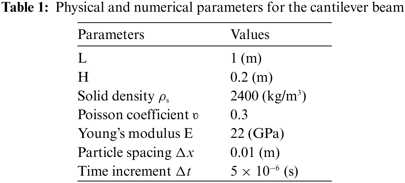
The concentrated load is represented by F, and the bending and shear stiffnesses are represented separately by EI and GA.

As shown in Fig. 6, the displacement fields calculated by the near-field dynamic model and the finite element calculation model are compared to the concentrated load of the two-dimensional cantilever beam. It can be observed that the displacement fields obtained by the two methods are consistent.

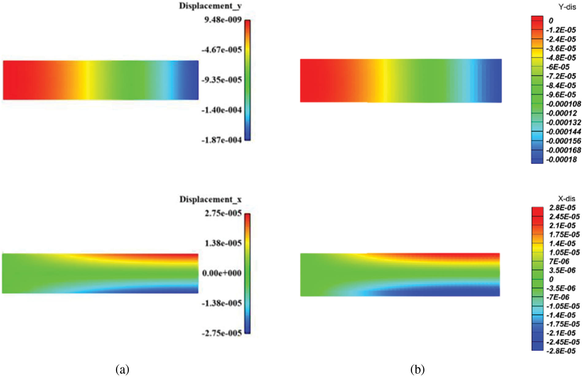
Figure 6: (a) horizontal and vertical displacements given by FEM [43], (b) the corresponding peridynamics results

It can be concluded that the NOSB-PD structure solver proposed in this study can qualitatively and quantitatively simulate the elastic solid problem. Hence, this structure solver will be used later in the fluid-structure interaction model.

4.2 Water Column Collapse Problem in a Tank

The ULPH solver is validated by simulating the famous water column collapse problem in a tank. The length and height of the water column are taken as L = H = 57 mm, while the tank’s length is 4H. The geometric model of the problem is the same as in Sun et al.'s work [44], as shown in Fig. 7. Both sides and bottom boundaries are slip-free; the relevant parameters are shown in Table 2.

Figure 7: Initial geometric configuration of the water column collapse problem in a tank

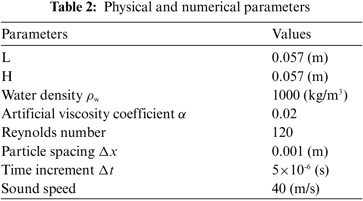
Fig. 8 shows the contour map of the pressure field every 0.1 s. At each instance, the ULPH solver accurately captures the pressure gradient distribution and the surface profile of the water before and after hitting the left solid wall boundary. The solver is also highly consistent compared to the results of SPH [44,45]. It can be seen that the pressure field and free surface profile of the current ULPH algorithm pressure simulation agree with the simulation results by Rahimi et al. [45]. A further comparison of the water flow is also given in Fig. 9. The graph in this figure shows the non-dimensional horizontal change of the waterfront toe.

Figure 8: Contour plot of the pressure field and surface evolution of the fluid by: (a) ULPH, and (b) SPH [45]

Figure 9: Comparison of the simulated and tested [45] time evolution of the waterfront

4.3 A Sloshing Tank

The ULPH single-phase flow model is utilized to investigate the tank sloshing problem in this section. The model parameters of the numerical example are set according to the experiment of Faltinsen et al. [46] The length of the rectangular tank is L = 1.73 m, the height is D = 1.15 m, and the water depth in the tank is H = 0.5 m at the initial time, as shown in Fig. 10. At the free surface, a measurement point FS1 is set at 0.05 m from the left wall of the liquid tank, which is used to record the evolution of the water surface height over time. The fluid density in the rectangular tank is ρ = 1000 kg/m3, and the gravitational acceleration is g = 9.81 m/s2. The Reynolds number is 120, the speed of sound is 30 m/s, and α is 0.1. The rectangular liquid tank is excited by a regular sinusoidal excitation in the horizontal direction (x-axis). The motion velocity of the rectangular liquid tank [47] is:

{u(t)=−2πTA0sin⁡(2πTt)v(t)=0,(60)

where A0 = 0.032 m is the amplitude and T = 1.875 s is the period. The initial particle spacing of the computational domain is Δx = 0.01 m. This example is simulated for 6 s, and the reference sound speed is set to c0 = 40 m/s.

Figure 10: Sketch of the initial setup of the sloshing tank

Fig. 11 shows the evolution of the sloshing liquid level and the distribution of the pressure field in the tank at different times under horizontal excitation. The tank moves back and forth in the horizontal direction under periodic external excitation, causing the water in the tank to move back and forth and produce large liquid surface deformation. The water pressure field in the figure is smooth, without pressure oscillation. Moreover, the distribution of particles at the liquid surface is continuous, without non-physical gaps. Therefore, the stability and accuracy of the ULPH fluid model when simulating large deformation-free surface flow problems can be confirmed.

Figure 11: The development of the free surface and pressure field distribution of the rectangular tank sloshing at different times under horizontal excitation

Fig. 12 shows the evolution of the water surface height at the measured point over time and compares it with the experimental results of Faltinsen et al. [46]. It can be seen that the ULPH measured results agree with the experimental data.

Figure 12: The change of the water surface height with time at the measurement point FS1

4.4 Breaking Dam Impacting on An Elastic Plate

Dam-break flows impacting elastic plates are modeled to demonstrate the effectiveness of the FSI framework proposed in this work for violent free-surface flows interacting with deformable structures. Dam-break plates have been extensively simulated as an appropriate benchmark to validate numerical models of FSI problems [44,45,48,49].

Fig. 13 shows the initial appearance of this model, with water of width L and height 2L initially located on the left and bottom walls. The distance between the two vertical walls is 4L. An elastic baffle is fixed at the bottom end at a distance of L from the water column; the top of the baffle is free, and the bottom is fixed. The water column collapses rapidly and rushes towards the right boundary under the force of gravity. Strong FSI occurs when the flow front collides with the baffle. In this case, baffles are considered as ideal elastomers. The material and fluid parameters of the baffle are shown in Table 3.

Figure 13: Geometric configuration of the water impact on an elastic plate

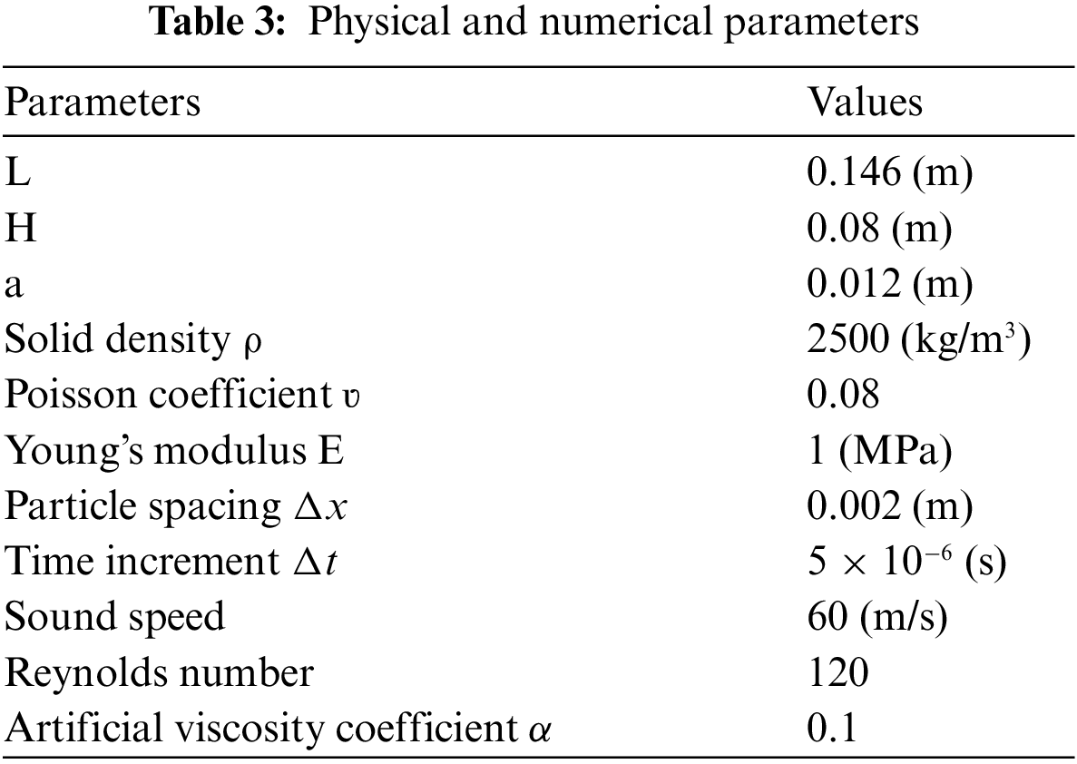
Fig. 14 shows the simulation of the dam-break flow impacting the baffles, the fluid’s pressure distribution, and the structure’s deformation obtained using other numerical models. The results show that the coupled model successfully reproduces the pressure field and structural deformation near the fluid-solid interface. Moreover, the flow state, pressure distribution, and structural deformation are consistent with the results of SPH-PD [44,45,48,49] simulation and PFEM [50] simulation.

Figure 14: Dam break flow impacting the baffle based on different numerical models

Fig. 15 shows the evolution of the horizontal displacement of the free end of the baffle, i.e., point A in Fig. 13. Once the wavefront of the burst dam reaches the elastic plate, the pressure at the lower part of the fluid-elastic plate interaction area increases rapidly, maximizing the elastic plate deflector. At this stage (0.15–0.23 s), the free end of the elastic plate undergoes high-speed deformation. As the fluid moves on the plate, its deflection decreases with the fluid pressure, followed by a rebound. The water column flowing down the baffle eventually hits the vertical wall on the right side. Here, the impact on the hard wall produces a violent splash, undergoes a regional instantaneous pressure increase, and finally gradually falls due to gravity.

Figure 15: Comparison of the predicted evolution of the horizontal displacement of point A based on different numerical models [44,45,48–50]

The Drucker-Prager model [51] was introduced into the solid solver established by NOSB-PD to simulate the impact of water flow on the geotechnical baffler and consider the damage problem of the solid in the solid constitution in the previous section with a critical bond stretch ratio of s0 = 0.069. The simulation’s other parameters were identical to [52]. The parameters in the Drucker-Prager constitutive are given in Table 4. Fig. 16 shows simulation snapshots of the dam-break flow propagation and the brittle fracturing of the baffle. The pressure distribution in the water and the displacement in the x-direction field near the baffle were obtained.

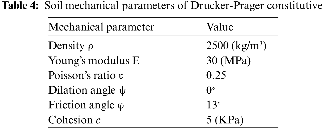
Figure 16: Snapshot of the pressure and displacement in the x-direction obtained by the proposed method

4.5 Interaction of a Dam-Break Wave with an Elastic Sluice Gate

The second FSI validation example for the ULPH-PD coupled model is the interaction between the dam-break flow and the elastic gate, first investigated experimentally and numerically by Yilmaz et al. [53]. The initial geometry of the model is shown in Fig. 17. The height of the water column is 0.2 m, and the width is 0.5 m. The water column is initially in a static state. An elastic gate is placed 0.3 m away from the water column; the length of the elastic gate is 0.125 m, and the width is 0.007 m. The material and specific fluid parameters of the elastic gate are shown in Table 5.

Figure 17: Geometric configuration of the interaction between a dam-break wave and an elastic sluice gate

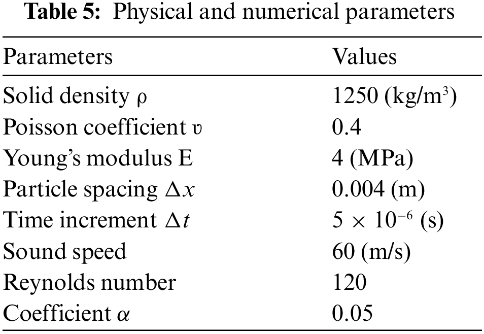
Fig. 18 compares the results of the PD-ULPH coupled model of this problem with the experimental results. The PD-ULPH model can predict the water-free surface’s position and the elastic gate’s deformation. Moreover, the pressure field and horizontal displacement field are also smooth. At t = 0 s, the solid wall on the right is released, and the water column collapses. After 0.2 s, the fluid starts to impact the elastic gate, and the outlet formed by the hydraulic pressure of the elastic gate gradually increases. The outlet gradually decreases with water pressure when it reaches the maximum value.

Figure 18: Comparison frames of the experimental [53] and numerical results at various time steps

Fig. 19 shows the horizontal displacement comparison at measurement point A. The coupled simulation results agree with the experimental measurement data [53].

Figure 19: Time histories of horizontal displacements at the measurement point A

4.6 Dam Break Flow through an Elastic Gate

A dam-break flow through an elastic gate is a classic FSI validation case. Antoci et al. [54] investigated this experimentally and numerically, including the configuration and elastic deformation of the dam-break flow. In addition, other numerical models investigated this case, such as the SPH-PD model [43,44].

Fig. 20 illustrates the initial geometry of this model. The water column is initially stationary, and an elastic plate is placed at the outlet with the top end fixed and the lower end free. The plate deforms, and the water column starts to collapse due to the hydrostatic pressure applied by the water column. Then, the water flows through the gate to the right boundary. The geometric and configuration parameters are shown in Table 6.

Figure 20: Model configuration for the dam break test through an elastic gate

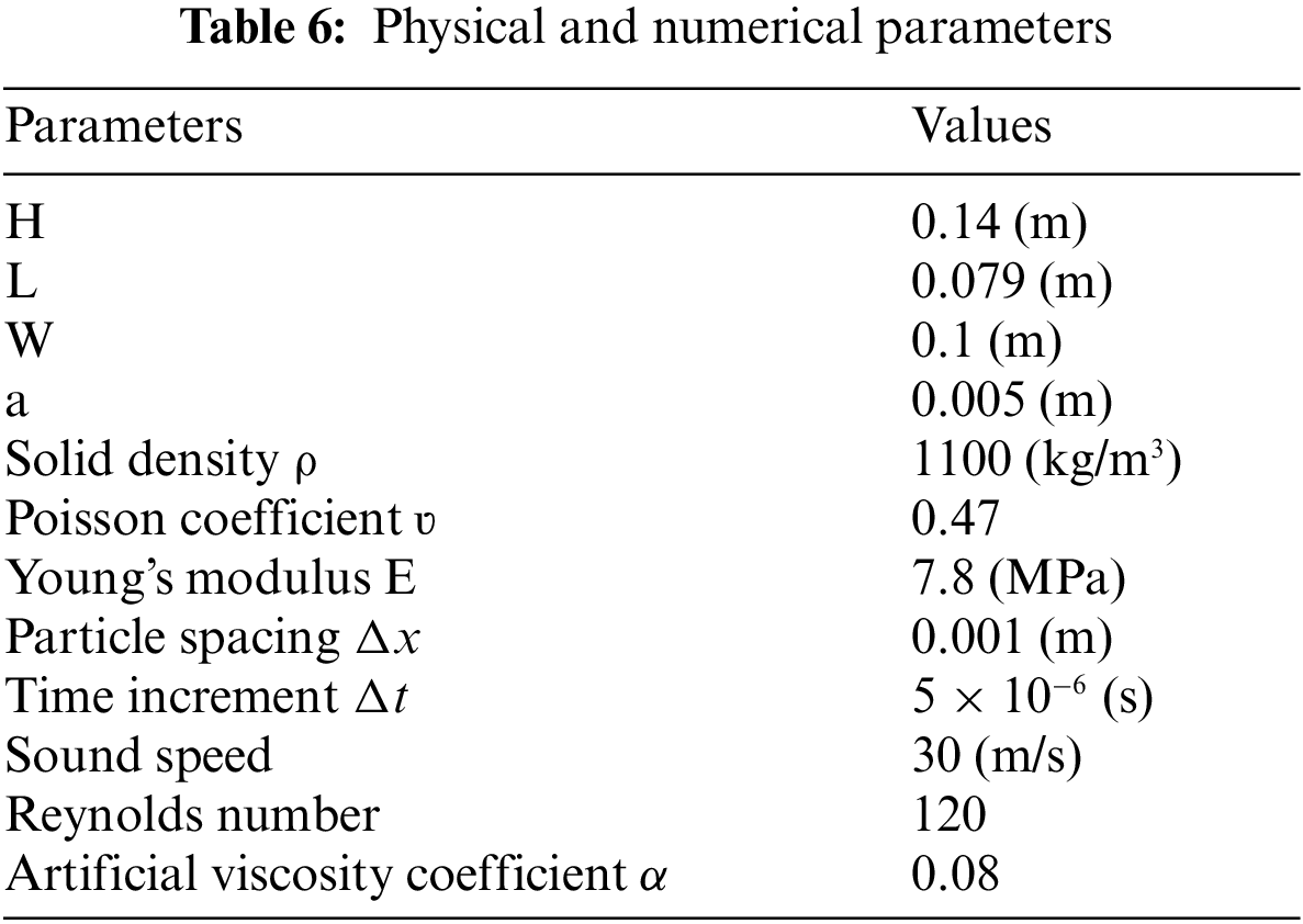
Fig. 21 compares the numerical results of the proposed ULPH-PD model with the experimental results previously published by Antoci et al. [54]. The fluid’s pressure contours and the elastic gate’s displacement field are plotted. The proposed model accurately reproduces the experimental process, including the evolution of the water level and the deformation of the elastic gate. Furthermore, the pressure and horizontal displacement fields are also smooth. In the simulation, the high-pressure point is mainly located in the lower right corner of the water tank and the narrow outlet at the bottom of the elastic plate. In addition, the water outlet formed by the elastic plate due to water pressure is also gradually reduced due to the gradual decrease of water pressure and the rebound of the elastic plate. Moreover, the horizontal and vertical displacements at the bottom of the elastic plate are presented in Fig. 22 and compared with experimental and other simulation results. Good agreement between the current results and experiments indicates better performance of the proposed ULPH-PD model in dealing with the FSI problem.

Figure 21: comparison of experimental photographs [54] with snapshots of the proposed numerical model

Figure 22: Comparison of displacements at the bottom center point of the elastic gate with different coupling approaches [43,44,54–56]: (a) horizontal displacement, and (b) vertical displacement

5  Conclusions

The FSI problem was modeled using two grid-free methods in this study–the recently developed Updated Lagrangian Particle Hydrodynamics (ULPH) method and the Non-Ordinary State-Based Peridynamics (NOSB-PD) method. The fluid and solid phases were modeled by NOSB-PD and ULPH respectively in this numerical framework. The two solvers were coupled by partition coupling, solving the interaction problem between the fluid and the deformable structure. Since ULPH was proposed based on the PD and combined with SPH, both have similarities in non-locality and form and unique advantages in fluid-structure interaction problems.

In the validation phase, the fluid solver modeled using ULPH was validated through two benchmark cases: The water column collapse problem in the tank and the liquid tank sloshing problem. A benchmark test of a cantilever subjected to a concentrated force at one end was performed to verify the accuracy of the solid solver modeled using NOSB-PD. Moreover, the model’s accuracy was verified according to the load-deflection results. Then, FSI benchmarks without failure were performed, including dam-break flow impacting the elastic plate, dam-break through an elastic gate, and dam-break flow impacting the elastic gate. The simulation results agree with other sources’ experimental and numerical results regarding structure deformation and flow pattern. In addition, the pressure and displacement fields are also quite smooth, indicating that the proposed ULPH-PD method is accurate and reliable. Finally, the Drucker-Prager constitutive model was used in the NOSB-PD model and applied to the problem of dam-break flow impacting the elastic plate. The model was used to solve and analyze the FSI problem with structural deformation and failure.

The proposed FSI solver requires further enhancement to adapt to practical engineering applications. Suitable turbulence models should be developed for fluid solvers, while solid solvers should simulate the deformation and failure of complex solid structures, so the advantages of non-ordinary state-based peridynamics should be combined with the constitutive under classical continuum mechanics for further study.

Acknowledgement: The authors are grateful to the anonymous reviewers for improving this article.

Funding Statement: The authors would like to thank the open foundation of the Hubei Key Laboratory of Theory and Application of Advanced Materials Mechanics and the Open Foundation of Hubei Key Laboratory of Engineering Structural Analysis and Safety Assessment.

Author Contributions: The authors confirm contribution to the paper as follows: study conception and design: Zhen Wang, Xin Lai; data collection: Zhen Wang, Junsong Xiong; analysis and interpretation of results: Zhen Wang; draft manuscript preparation: Zhen Wang; management and coordination: Xin Lai, Shaofan Li, Xiang Liu, Lisheng Liu. All authors reviewed the results and approved the final version of the manuscript.

Availability of Data and Materials: The data and related programs are available from the first and corresponding authors upon reasonable request.

Conflicts of Interest: The authors declare that they have no conflicts of interest to report regarding the present study.

References

1. Zhang Z, Hui L, Zhu S, Zhao F. Application of CFD in ship engineering design practice and ship hydrodynamics. J Hydrodyn Ser B. 2006;18(3):315–22. doi:10.1016/S1001-6058(06)60072-3. [Google Scholar] [CrossRef]

2. Wang JH, Wan DC. CFD simulation of ship turning motion in waves. Chin J Ship Res. 2019;14(1):1–8. [Google Scholar]

3. Zhang AM, Wang SP, Peng YX, Ming F, Liu YL. Research progress in underwater explosion and its dam-age to ship structures. Chin J Ship Res. 2019;14(3):1–13 (In Chinese). [Google Scholar]

4. Lai X, Li S. Substrate elasticity and surface tension mediate the spontaneous rotation of active chiral droplet on soft substrates. J Mech Phys Solids. 2022;161(5):104788. doi:10.1016/j.jmps.2022.104788. [Google Scholar] [CrossRef]

5. Hirt CW, Nichols BD. Volume of fluid (VOF) method for the dynamics of free boundaries. J Comput Phys. 1981;39(1):201–25. doi:10.1016/0021-9991(81)90145-5. [Google Scholar] [CrossRef]

6. Raeini AQ, Blunt MJ, Bijeljic B. Modelling two-phase flow in porous media at the pore scale using the volume-of-fluid method. J Comput Phys. 2012;17(17):5653–68. doi:10.1016/j.jcp.2012.04.011. [Google Scholar] [CrossRef]

7. Sussman M, Smereka P, Osher S. A level set approach for computing solutions to incompressible two-phase flow. J Comput Phys. 1994;114(1):146–59. doi:10.1006/jcph.1994.1155. [Google Scholar] [CrossRef]

8. Osher S, Fedkiw RP. Level set methods: an overview and some recent results. J Comput Phys. 2001;169(2):463–502. doi:10.1006/jcph.2000.6636. [Google Scholar] [CrossRef]

9. Chen S, Doolen GD. Lattice Boltzmann method for fluid flows. Annu Rev Fluid Mech. 1998;30(1):329–64. doi:10.1146/annurev.fluid.30.1.329. [Google Scholar] [CrossRef]

10. Chen GQ, Zhang AM, Huang X. On the interaction between bubbles and the free surface with high density ratio 3D lattice Boltzmann method. Theor Appl Mech Lett. 2018;8(4):252–6. doi:10.1016/j.taml.2018.04.006. [Google Scholar] [CrossRef]

11. Unverdi SO, Tryggvason G. A front-tracking method for viscous, incompressible, multi-fluid flows. J Comput Phys. 1992;100(1):25–37. doi:10.1016/0021-9991(92)90307-K. [Google Scholar] [CrossRef]

12. Tryggvason G, Bunner B, Esmaeeli A, Juric D, Al-Rawahi N. A front-tracking method for the computations of multiphase flow. J Comput Phys. 2001;169(2):708–59. doi:10.1006/jcph.2001.6726. [Google Scholar] [CrossRef]

13. Monaghan JJ. Simulating free surface flows with SPH. J Comput Phys. 1994;110(2):399–406. doi:10.1006/jcph.1994.1034. [Google Scholar] [CrossRef]

14. Liu WK, Jun S, Sihling DT, Chen YJ, Hao W. Multiresolution reproducing kernel particle method for computational fluid dynamics. Int J Numer Methods Fluids. 1997;24(12):1391–415. doi:10.1002/(SICI)1097-0363(199706)24:12<1391::AID-FLD566>3.0.CO;2-2. [Google Scholar] [CrossRef]

15. Xie F, Zhao W, Wan D. Overview of moving particle semi-implicit techniques for hydrodynamic problems in ocean engineering. J Mar Sci Appl. 2022;21(3):1–22. doi:10.1007/s11804-022-00284-9. [Google Scholar] [CrossRef]

16. Zhang DZ, Zou Q, VanderHeyden WB, Ma X. Material point method applied to multiphase flows. J Comput Phys. 2008;227(6):3159–73. doi:10.1016/j.jcp.2007.11.021. [Google Scholar] [CrossRef]

17. Tu Q, Li S. An updated Lagrangian particle hydrodynamics (ULPH) for Newtonian fluids. J Comput Phys. 2017;348:493–513. doi:10.1016/j.jcp.2017.07.031. [Google Scholar] [CrossRef]

18. Liu MB, Li S. On the modeling of viscous incompressible flows with smoothed particle hydrodynamics. J Hydrodyn. 2016;28(5):731–45. doi:10.1016/S1001-6058(16)60676-5. [Google Scholar] [CrossRef]

19. Bergel GL, Li S. The total and updated lagrangian formulations of state-based peridynamics. Comput Mech. 2016;58:351–70. doi:10.1007/s00466-016-1297-8. [Google Scholar] [CrossRef]

20. Oñate E, Carbonell JM. Updated lagrangian mixed finite element formulation for quasi and fully incompressible fluids. Comput Mech. 2014;54:1583–96. doi:10.1007/s00466-014-1078-1. [Google Scholar] [CrossRef]

21. Silling SA. Reformulation of elasticity theory for discontinuities and long-range forces. J Mech Phys Solids. 2000;48(1):175–209. doi:10.1016/S0022-5096(99)00029-0. [Google Scholar] [CrossRef]

22. Silling SA, Epton M, Weckner O, Xu J, Askari E. Peridynamic states and constitutive modeling. J Elast. 2007;88(2):151–84. doi:10.1007/s10659-007-9125-1. [Google Scholar] [CrossRef]

23. Silling SA, Lehoucq RB. Peridynamic theory of solid mechanics. Adv Appl Mech. 2010;44:73–168. doi:10.1016/S0065-2156(10)44002-8. [Google Scholar] [CrossRef]

24. Zhou XP, Wang YT, Shou YD. Hydromechanical bond-based peridynamic model for pressurized and fluid-driven fracturing processes in fissured porous rocks. Int J Rock Mech Min Sci. 2020;132(6134):104383. doi:10.1016/j.ijrmms.2020.104383. [Google Scholar] [CrossRef]

25. Liu R, Yan J, Li S. Modeling and simulation of ice-water interactions by coupling peridynamics with updated Lagrangian particle hydrodynamics. Comput Part Mech. 2019;7(2):241–55. doi:10.1007/s40571-019-00268-7. [Google Scholar] [CrossRef]

26. Yan J, Li S, Kan X, Zhang AM, Lai X. Higher-order non-local theory of updated lagrangian particle hydrodynamics (ULPH) and simulations of multiphase flows. Comput Methods Appl Mech Eng. 2020;368:113176. [Google Scholar]

27. Yan J, Li S, Zhang AM, Kan XY, Sun PN. Updated lagrangian particle hydrodynamics (ULPH) modeling and simulation of multiphase flows. J Comput Phys. 2019;393:406–37. [Google Scholar]

28. Yan J, Li S, Kan X, Lv P, Zhang AM. Updated Lagrangian particle hydrodynamics (ULPH) modeling for free-surface fluid flows. Comput Mech. 2024;73(2):297–316. [Google Scholar]

29. Colagrossi A, Souto-Iglesias A, Antuono M, Marrone S. Smoothed-particle-hydrodynamics modeling of dissipation mechanisms in gravity waves. Phys Rev E. 2013;87(2):023302. [Google Scholar]

30. Molteni D, Colagrossi A. A simple procedure to improve the pressure evaluation in hydrodynamic context using the SPH. Comput Phys Commun. 2009;180(6):861–72. [Google Scholar]

31. Yan J, Li S, Kan X, Zhang AM, Liu L. Updated Lagrangian particle hydrodynamics (ULPH) modeling of solid object water entry problems. Comput Mech. 2021;67(6):1685–703. doi:10.1007/s00466-021-02014-4. [Google Scholar] [CrossRef]

32. Colagrossi A, Landrini M. Numerical simulation of interfacial flows by smoothed particle hydrodynamics. J Comput Phys. 2003;191(2):448475. doi:10.1016/S0021-9991(03)00324-3. [Google Scholar] [CrossRef]

33. Belytschko T, Liu WK, Moran B, Elkhodary K. Nonlinear finite elements for continua and structures. Germany: JohnWiley & Sons; 2014. [Google Scholar]

34. Zhou XP, Tian DL. A novel linear elastic constitutive model for continuum-kinematics-inspired peridynamics. Comput Methods Appl Mech Eng. 2021;373(1):113479. doi:10.1016/j.cma.2020.113479. [Google Scholar] [CrossRef]

35. Lai X, Ren B, Fan H, Li S, Wu C, Liu L. Peridynamics simulations of geomaterial fragmentation by impulse loads. Int J Numer Anal Methods Geomech. 2015;39(12):1304–30. doi:10.1002/nag.2356. [Google Scholar] [CrossRef]

36. Hughes TJR, Winget J. Finite rotation effects in numerical integration of rate constitutive equations arising in large-deformation analysis. Int J Numer Methods Eng. 1980;15(12):1862–7. doi:10.1002/nme.1620151210. [Google Scholar] [CrossRef]

37. Huang D, Lu G, Wang C, Qiao P. An extended peridynamic approach for deformation and fracture analysis. Eng Fract Mech. 2015;141(8):196–211. doi:10.1016/j.engfracmech.2015.04.036. [Google Scholar] [CrossRef]

38. Lai X, Liu L, Li S, Migbar Z, Liu Q, Wang Z. A non-ordinary state-based peridynamics modeling of fractures in quasi-brittle materials. Int J Impact Eng. 2018;111(1):130–46. doi:10.1016/j.ijimpeng.2017.08.008. [Google Scholar] [CrossRef]

39. Silling SA, Askari E. A meshfree method based on the peridynamic model of solid mechanics. Comput Struct. 2005;83(17–18):1526–35. doi:10.1016/j.compstruc.2004.11.026. [Google Scholar] [CrossRef]

40. Adami S, Hu XY, Adams NA. A generalized wall boundary condition for smoothed particle hydrodynamics. J Comput Phys. 2012;231(21):7057–75. doi:10.1016/j.jcp.2012.05.005. [Google Scholar] [CrossRef]

41. Sun P, Ming F, Zhang A. Numerical simulation of interactions between free surface and rigid body using a robust SPH method. Ocean Eng. 2015;98(21):32–49. doi:10.1016/j.oceaneng.2015.01.019. [Google Scholar] [CrossRef]

42. Bouscasse B, Colagrossi A, Marrone S, Antuono M. Nonlinear water wave interaction with floating bodies in SPH. J Fluid Struct. 2013;42(8):112–29. doi:10.1016/j.jfluidstructs.2013.05.010. [Google Scholar] [CrossRef]

43. Yao X, Huang D. Coupled PD-SPH modeling for fluid-structure interaction problems with large deformation and fracturing. Comput Struct. 2022;270:106847. doi:10.1016/j.compstruc.2022.106847. [Google Scholar] [CrossRef]

44. Sun WK, Zhang LW, Liew KM. A smoothed particle hydrodynamics peridynamics coupling strategy for modeling fluid-structure interaction problems. Comput Methods Appl Mech Eng. 2020;371:113298. doi:10.1016/j.cma.2020.113298. [Google Scholar] [CrossRef]

45. Rahimi MN, Kolukisa DC, Yildiz M, Ozbulut M, Kefal A. A generalized hybrid smoothed particle hydrodynamics-peridynamics algorithm with a novel Lagrangian mapping for solution and failure analysis of fluid-structure interaction problems. Comput Methods Appl Mech Eng. 2022;389(1–3):114370. doi:10.1016/j.cma.2021.114370. [Google Scholar] [CrossRef]

46. Faltinsen OM, Rognebakke OF, Lukovsky IA, Timokha AN. Multidimensional modal analysis of nonlinear sloshing in a rectangular tank with finite water depth. J Fluid Mech. 2000;407:201–34. doi:10.1017/S0022112099007569. [Google Scholar] [CrossRef]

47. Wang PP, Meng ZF, Zhang AM, Ming FR, Sun PN. Improved particle shifting technology and optimized free-surface detection method for free-surface flows in smoothed particle hydrodynamics. Comput Methods Appl Mech Eng. 2019;357(2):112580. doi:10.1016/j.cma.2019.112580. [Google Scholar] [CrossRef]

48. Dai Z, Xie J, Jiang M. A coupled peridynamics-smoothed particle hydrodynamics model for fracture analysis of fluid-structure interactions. Ocean Eng. 2023;279(3):114582. doi:10.1016/j.oceaneng.2023.114582. [Google Scholar] [CrossRef]

49. Sun WK, Zhang LW, Liew KM. A coupled SPH-PD model for fluid-structure interaction in an irregular channel flow considering the structural failure. Comput Methods Appl Mech Eng. 2022;401:115573. doi:10.1016/j.cma.2022.115573. [Google Scholar] [CrossRef]

50. Idelsohn SR, Marti J, Limache A, Oñate E. Unified Lagrangian formulation for elastic solids and incompressible fluids: application to fluid-structure interaction problems via the PFEM. Comput Methods Appl Mech Eng. 2008;197(19–20):1762–76. doi:10.1016/j.cma.2007.06.004. [Google Scholar] [CrossRef]

51. Drucker DC, Prager W. Soil mechanics and plastic analysis or limit design. Q Appl Math. 1952;10(2):157–65. doi:10.1090/qam/48291. [Google Scholar] [CrossRef]

52. Feng K, Huang D, Wang G, Jin F, Chen Z. Physics-based large-deformation analysis of coseismic landslides: a multiscale 3D SEM-MPM framework with application to the Hongshiyan landslide. Eng Geol. 2022;297:106487. [Google Scholar]

53. Yilmaz A, Kocaman S, Demirci M. Numerical modeling of the dam-break wave impact on elastic sluice gate: a new benchmark case for hydroelasticity problems. Ocean Eng. 2021;231:108870. [Google Scholar]

54. Antoci C, Gallati M, Sibilla S. Numerical simulation of fluid-structure interaction by SPH. Comput Struct. 2007;85(11–14):879–90. [Google Scholar]

55. Khayyer A, Gotoh H, Falahaty H, Shimizu Y. An enhanced ISPH-SPH coupled method for simulation of incompressible fluid-elastic structure interactions. Comput Phys Commun. 2018;232:139–64. [Google Scholar]

56. Zhang C, Rezavand M, Hu X. A multi-resolution SPH method for fluid-structure interactions. J Comput Phys. 2021;429:110028. [Google Scholar]