Determination of the Pile Drivability Using Random Forest Optimized by Particle Swarm Optimization and Bayesian Optimizer

1  Introduction

The role of piles is often to transfer structural loads from the upper to the lower geotechnical layers through the formation media in most engineering environments. Pile driving usually involves hammering, where the impact forces can generate tensile and compressive stresses within the pile. When these stresses exceed the resistance strength of the pile materials, it may lead to fracture or damage of the pile [1,2]. Therefore, maximum tensile stress (MTS), maximum compressive stress (MCS), and blows per foot (BPF) are critical technical parameters that must be carefully considered during pile design and driving processes [3,4]. By predicting these parameters through calculations in the design phase, the design of the piles can be effectively optimized, achieving a construction that is both safe and economical.

In early engineering practices, the driving behaviour of piles was often predicted based on the point mass model from Newtonian mechanics. However, this method, which overlooks many practical factors, has limited accuracy. In 1931, Isaac [5] discovered that energy is transmitted through the propagation of impact stress waves in the hammer assembly and the pile, which fundamentally differs from Newton’s point mass model. In 1960, Smith [6] employed the theory of stress waves to propose an empirical formula for predicting pile driving characteristics. Although this formula simplifies the pile into a series of discrete mass points, it ignores the pile’s lateral vibrations and the complex nonlinear behaviour of the soil. In 1990, Nath [7] introduced the finite element analysis technique using the “continuous method” for pile driving analysis. While theoretically providing a more detailed analysis, this approach faces challenges of time consumption and parameter calibration in large-scale engineering applications. Additionally, traditional methods of pile driving analysis exhibit many uncertainties and nonlinear responses [8–10], complicating and increasing the uncertainty in problem analysis. Therefore, it is necessary to develop more accurate predictive models, such as machine learning models. Machine learning involves learning from historical data and dynamically adjusting and refining algorithms based on the encountered data patterns rather than strictly adhering to predetermined static models. This not only enhances the stability of predictions but also improves accuracy.

In recent years, many researchers have utilized artificial intelligence (AI) algorithms [11–13] such as support vector machines (SVM) [14], artificial neural networks (ANN) [15–17], and propagation neural network (BPNN) [18] as effective solutions in geotechnical problems. These research methods have important guiding significance for engineering design. For example, Das et al. [19] predicted the bearing capacity of piles through the use of the ANN model. In addition, the SVM model was proposed by Kordjazi et al. [20] to evaluate the bearing capacity of the pile under axial load conditions. Later, Zhang et al. [21] evaluated the ultimate bearing capacity of the driven piles using back BPNN regression model and multivariate adaptive regression splines and performed performance comparisons on the developed methods [22]. Although machine learning has made significant progress in addressing geotechnical engineering issues, existing models still exhibit limitations under various environmental conditions. Training an ANN is often a time-consuming process, largely because it is difficult to predict at the outset which network structure and parameter configuration will yield the best performance [23]. Additionally, while SVM demonstrates good accuracy when handling large datasets, its computational speed can be slow when dealing with complex problems. Concurrently, the random forest (RF) algorithm is renowned for its robust capability to process and interpret complex and nonlinear interactions among variables, making it particularly suitable for solving complex engineering challenges that traditional methods struggle to address [24–26].

This study proposed an optimized RF method for the forecast of the MTS, MCS, and BPF associated with the drivability of the pile. In addition to the optimized RF model and for comparison purposes, other models have been constructed, including SVM, k-nearest neighbour (KNN), extreme gradient boosting, and decision tree (DT). The arrangement of this article is as follows. Section 2 introduces RF and optimization methods in detail and briefly describes XGBoost, KNN, support vector regression (SVR), and DT. Section 3 presents the definition of data and variables. In Section 4, the training process of the models and their comparisons will be given. Finally, the last section presents conclusions and recommendations for further research.

2  Methodology

2.1 Machine Learning Models

RF enhances model generalization and predictive accuracy through the integration of multiple Decision Trees (DTs) [27,28]. Within the RF model, each tree is trained on a randomly selected subset of samples and features from the original dataset. This randomness aids the model in better adapting to diverse data distributions, thereby improving the overall stability and performance of the model [29–31]. DTs utilize the Mean Squared Error (MSE) to select the optimal splitting point during training, continuing until no additional features are available or the minimum MSE is achieved. The final prediction result of the forest is obtained by averaging the predictions from all the trees, the formula is as follows:

Y¯(x)=1K∑i=1KYi(x)(1)

where Y¯ is the RF prediction result; K is the number of trees; Yi is the prediction result of the ith decision tree.

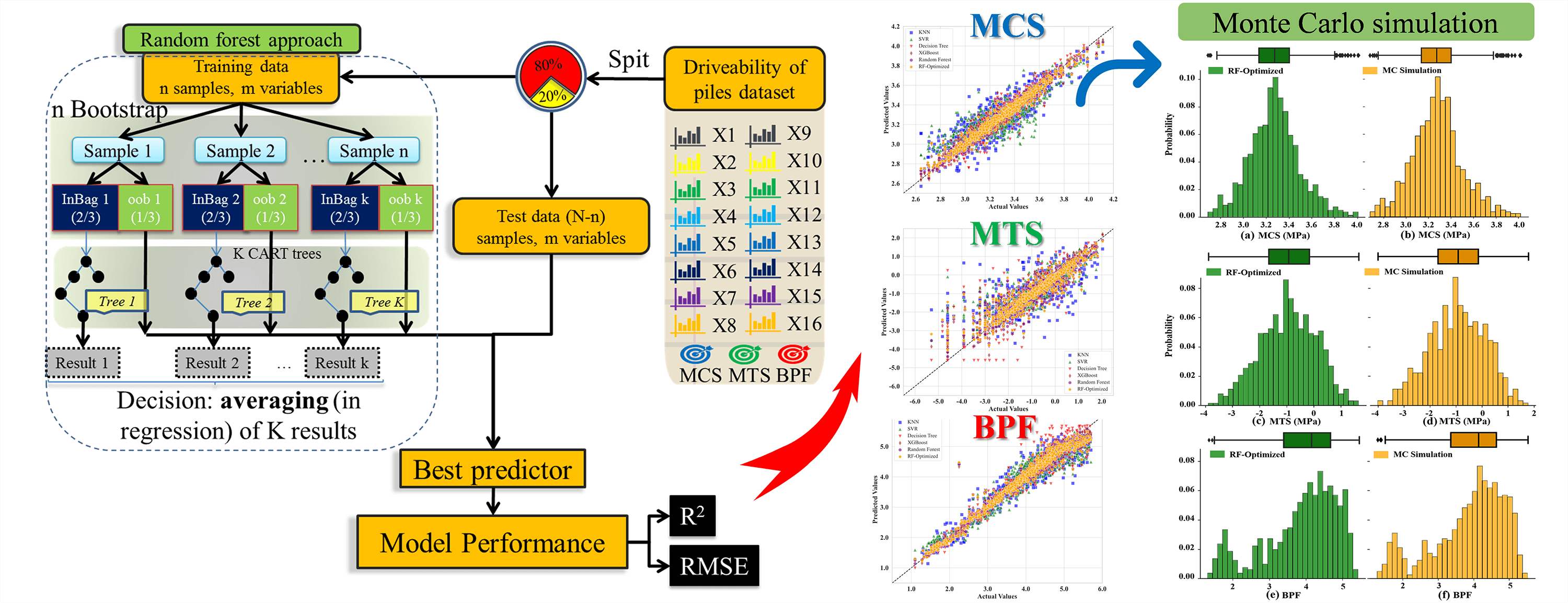
RF regression proves highly effective in analyzing nonlinear and collinear data, particularly as it does not require the assumption of a specific mathematical model form [31]. In this study, the RF model integrates multiple DTs to manage the diversity of pile drivability performance data, thus enabling the analysis and understanding of the drivability parameters of piles under various geological conditions. Fig. 1 illustrates the process of building the RF model in this study.

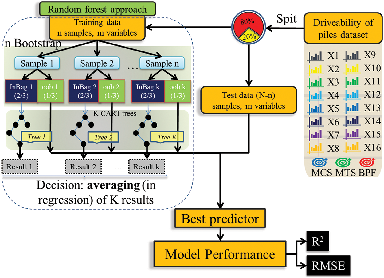
Figure 1: Flowchart of RF (RMSE: root mean square error)

In addition to the RF model, this study employs several commonly used regression methods to predict the drivability of piles, including XGBoost, DT, SVR, and KNN. For a detailed explanation of these models, readers are referred to previously published literature [32–35].

2.2 Particle Swarm Optimization

Particle Swarm Optimization (PSO), developed by Eberhart and Kennedy in 1995, is a metaheuristic optimization algorithm inspired by the foraging behaviour of birds. In PSO, each optimization problem is represented as a “particle” in the search space. Each particle possesses a fitness value determined by the objective function being optimized and a velocity dictating its direction and distance of movement. As the optimization progresses, particles adjust their movements to converge toward the current optimal solutions within the solution space. Suppose that Xi=(xi1,xi2,xi3,…,xin) represents the position vector of particle i, and Vi=(vi1,vi2,vi3,…,vin) represents the velocity vector of particle i [36,37], where n is the dimension size of the optimization problem. To have more control on the velocity, an inertia weight (W) can be described in the velocity equation [38]. Then, the speed vector iteration formula can be presented as follows [39–42]:

νi=Wνi+c1r1(Pbesti−xi)+c2r2(Gbesti−xi)(2)

xi=xi+νi(3)

In the above formulas, Pbesti and Gbesti represent the historical best position vector of particle i and the best position vector in the history of the population, the parameters c1 and c2 are called learning factors, and r1 and r2 are two random probability values distributed in [0,1], W is the inertia weight that is used to balance global and local search ability [43].

Through this mechanism, the PSO algorithm continuously learns from its own and the population’s historical information, optimizing the search process and gradually converging to the optimal solution. Additionally, the inertia weight w is an important parameter in PSO as it influences the velocity update and global search capability of the particles. In this study, the inertia weight w in the PSO algorithm was varied adaptively. Specifically, the inertia weight w decreases linearly during the iterations, starting from an initial value wmax = 0.9 and reducing to a final value wmin = 0.4. Fig. 2 illustrates the PSO optimization process.

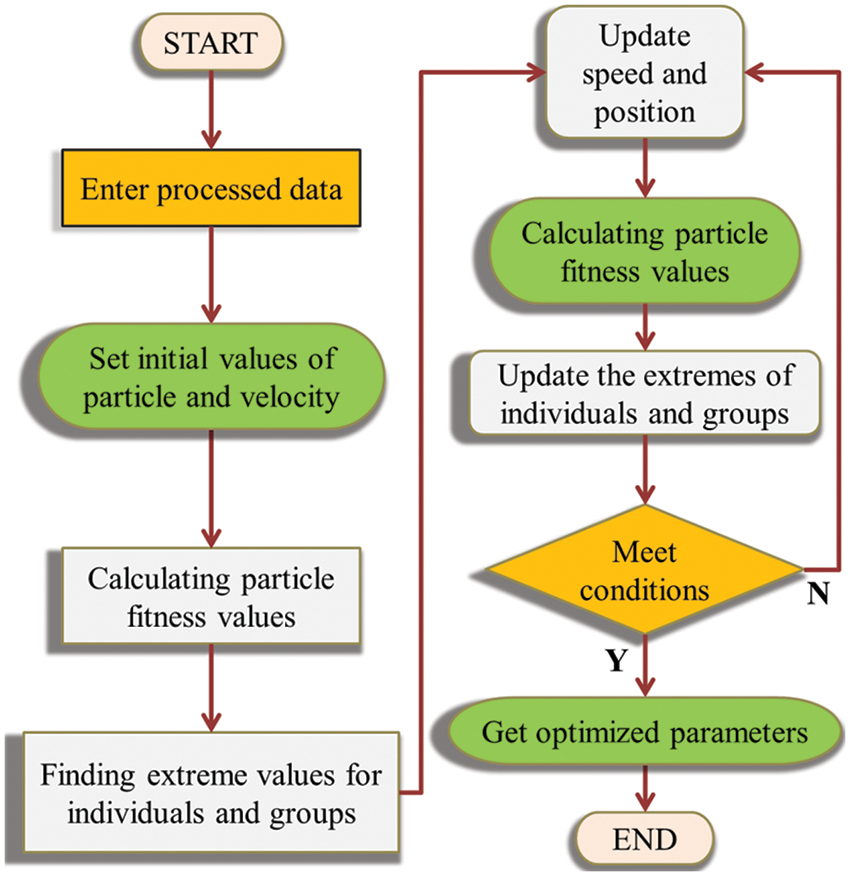
Figure 2: PSO optimization flowchart

2.3 Bayesian Optimization

Bayesian optimization (BO) differs from traditional gradient-based methods in that it uses a Gaussian process model to reveal the hidden relationships between hyper-parameters and the loss function. In the Bayesian tuning process, suppose a set of hyper-parameter combinations X=(x1,x2,…,xn) (xn represents the value of a hyper-parameter), and this set of hyper-parameters and the loss function f(x) that we need to optimize have a functional relationship [44]. When the value of x* is taken, the optimal Y=f(x∗) can be obtained. The first thing to mention is the fact that the Gaussian process is a normal distribution. It can then be assumed that this process of finding the optimal parameters is a Gaussian process [45,46]. The core steps of the BO algorithm are as follows: First, the sample point D={(Xt1,Yt2)} is used to estimate and update the Gaussian process f(x)∼GP(E(x),K(x,x,)). Then, the acquisition function EI(x) is then used to guide the new sampling.

EI(x)=(μ(x)−f(x+)−ξ)φ(Z)+σ(x)ϕ(Z)(4)

Z=μ(x)−f(x+)−ξσ(x)(5)

where φ is the cumulative distribution function of the standard normal distribution, ϕ is the probability density function of the standard normal distribution, and ξ is a non-negative parameter that controls the trade-off between exploration and exploitation.

BO, in principle, models the hidden relationship between hyperparameters and the loss function using a Gaussian process. This fitted function provides guidance on optimal parameters for the next iteration. By continuously adding sample points, the posterior distribution of the objective function is updated for a given optimized objective function [47,48]. For more comprehensive insights and discussions, other studies available in the literature can be found [49,50]. Fig. 3 illustrates the process of BO.

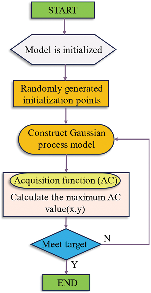
Figure 3: BO flowchart

3  Materials

3.1 Database for Modelling

This article collected a database of more than 4000 piles from the North Carolina project [51], which have been used in construction projects. The input of this database contains 17 characteristic parameters (concerning the information of hammer, hammer cushion material, pile information, and soil information), and the output is three target parameters (i.e., MCS, MTS, and BPF). The frequency distributions of the MCS, MTS, and BPF are shown in Fig. 4. It can be seen in Fig. 4 that MCS is approximately normally distributed, while MTS and BPF show skewed distributions and are skewed to the side where the data is small. The input and output parameters with their ranges are described in Table 1. Moreover, the correlation analysis between the influencing factors is also performed in Fig. 5. Fig. 5 shows the correlation coefficients between the variables. The closer the correlation coefficient is to 0, the worse the correlation between the two variables.

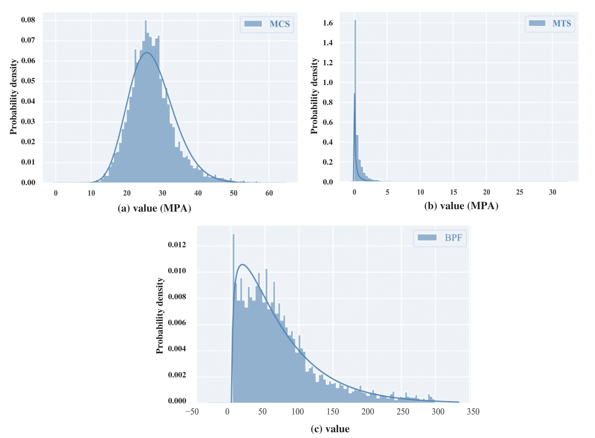
Figure 4: Frequency distribution of each output variable: (a) MCS data, (b) MTS data, and (c) BPF data

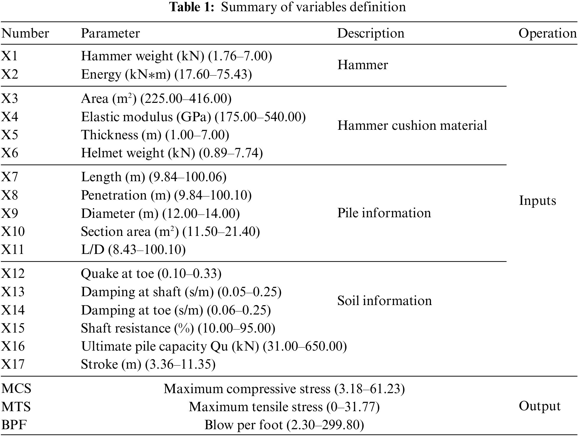
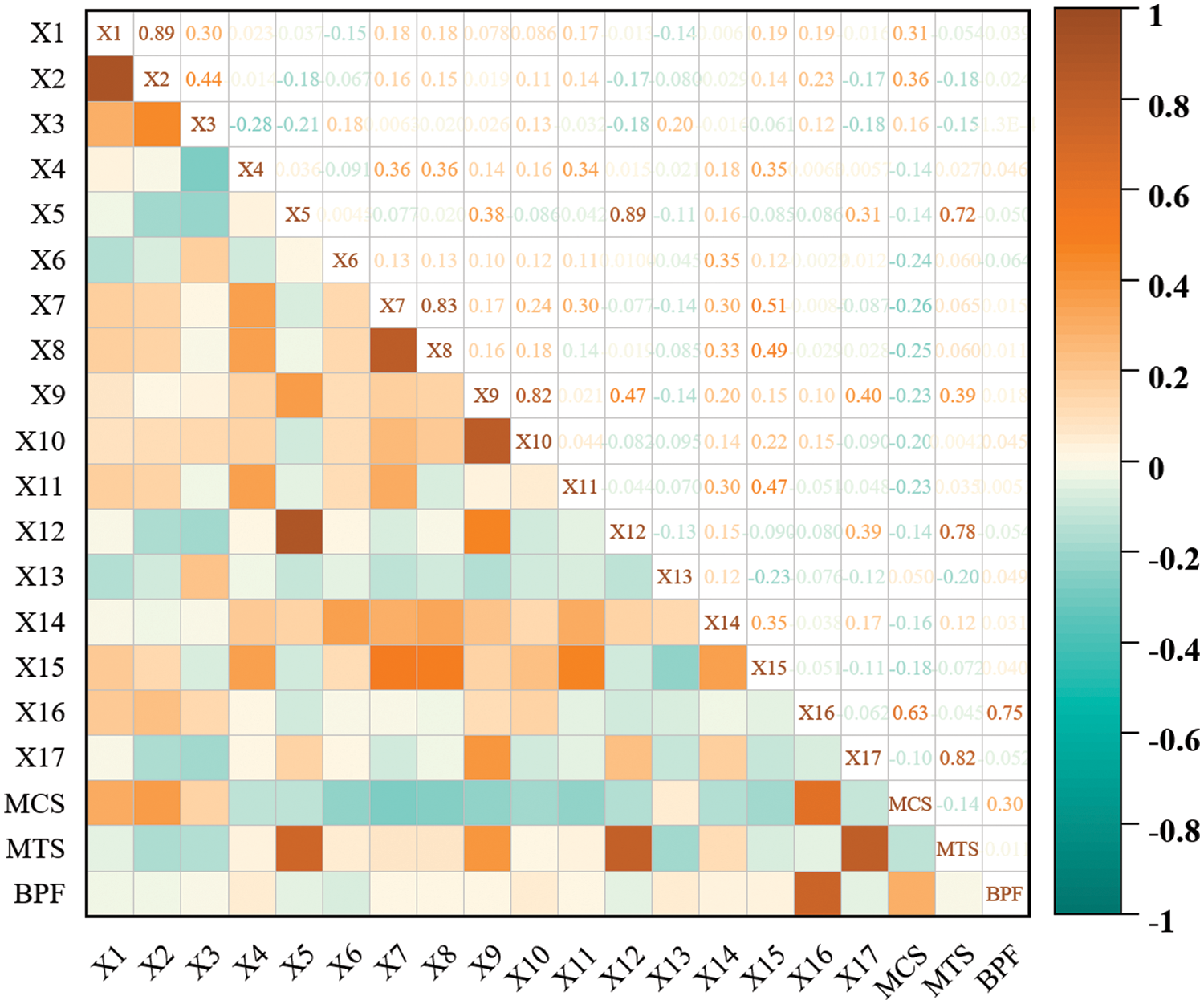
Figure 5: Correlation analysis between influencing factors

3.2 Performance Assessment

If the model’s training and test performance cannot be quantitatively evaluated, it is difficult to measure the quality of the model [52,53]. In general, the accuracy of the regression model is quantitatively evaluated by using indicators such as root mean square error (RMSE) and coefficient of determination (R2). In theory, when RMSE is equal to 0 and R2 is 1, the model is considered perfect. The RMSE is the square root of the ratio of the squared sum of deviation of the observed value to the true value and the number m of observations [54,55]. Use it to measure the deviation between predicted and true values. Therefore, the prediction ability of the model increases as the RMSE value decreases. The smaller the RMSE value, the better the prediction ability of the model. The R2 of the model is often used as a measure of the predictability of the model. The value of R2 represents the percentage of the square of the correlation between the predicted and actual values of the target variable. A model with an R2 value of 0 indicates that it is completely unpredictable for the target variable while a model with an R2 value of 1 can perfectly predict the target variable. The relevant equations of RMSE and R2 are as follows [56,57]:

RMSE=1N∑i=1N{}(yi^−yi)2(6)

R2=1−1N∑i=1N{}(yi−yi^)21N∑i=1N{}(yi−yi¯)2(7)

where yi represents the observed value, the yi^ is the predicted value of the model, yi¯ represents the average of the observed values, and N denotes the number of samples in the training or testing stages.

3.3 Models Development

In this study, various machine learning methods were employed to predict the drivability of piles. Following a performance comparison, several optimization techniques were applied to fine-tune the parameters of the RF model. The main modelling and optimization steps can be summarized as follows:

1.   Data preprocessing: Before model construction, relevant input parameters were selected through correlation assessment. For predicting different pile drivability parameters, the output variables underwent a logarithmic transformation, and missing values were removed. The constructed dataset comprised 4072 samples, with 80% allocated to the training set for model training and the remaining 20% assigned to the test set for model validation.

2.   Model construction: Initially, models were built without optimization, using default hyperparameters for RF, SVR, KNN, XGBoost, and DT. RMSE and the coefficient R² were selected as the performance evaluation metrics. Models were trained on the training set and evaluated on the test set, with performance metrics recorded for each model in their initial state.

3.   Hyperparameter optimization: BO and PSO methods were employed to optimize three hyperparameters of the RF model: the maximum number of features (max_feature), the number of estimators (n_estimators), and the minimum number of samples required to split an internal node (min_samples_split). The distribution of each hyperparameter during the optimization process was illustrated for the three prediction targets (MCS, MTS, and BPF).

4.   Model comparison: Using the optimized hyperparameter configurations, the models were retrained and tested. The optimized models were then compared with the initial models to analyze their performance, discuss their generalization capabilities, and evaluate their fit to the data.

4  Results and Discussion

In this section, the performance of the initial unoptimized models, including RF, SVR, KNN, XGBoost, and DT, is first evaluated to identify the best-performing model. Subsequently, BO and PSO are applied to fine-tune the hyperparameters of the selected optimal model. Finally, the performance of the optimized model is compared with the other models to determine the most effective model for predicting MCS, MTS, and BPF.

4.1 Predictive Performance of the Initial Model

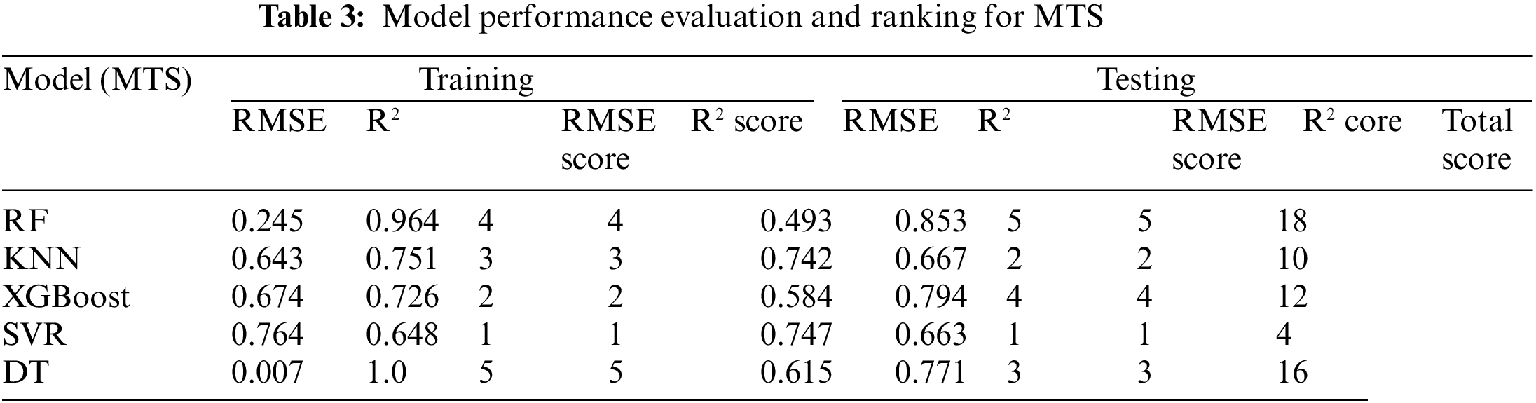
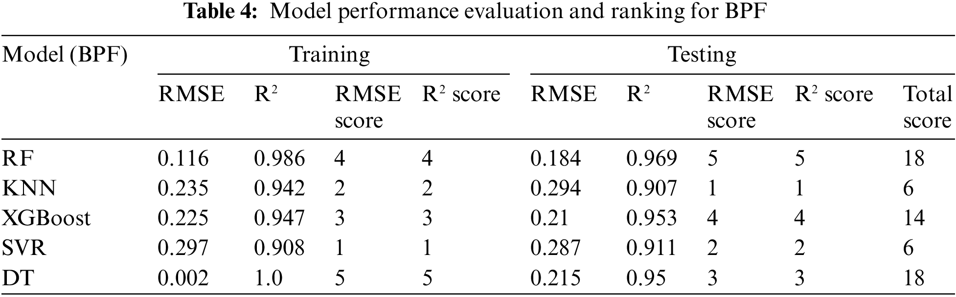
Tables 2–4 present the evaluation performance metrics, including R² and RMSE, for the constructed initial models predicting MCS, MTS, and BPF, respectively. Each model’s performance on the training and test sets was evaluated using a scoring system to identify the optimal model.

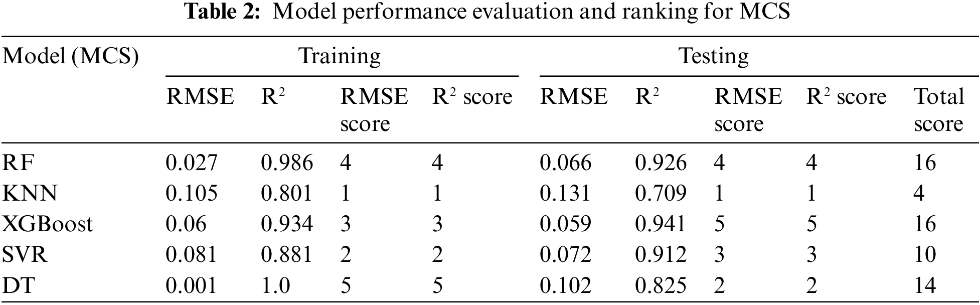
In predicting MCS, despite the DT model performing perfectly on the training set, its performance significantly declined on the test set (R² = 0.825, RMSE = 0.102), indicating a severe overfitting issue. The KNN model also showed poor performance on the test set in terms of R² and RMSE, suggesting its ineffectiveness in handling high-dimensional data. The XGBoost model achieved a relatively high R² (0.941) on the test set, but its overall score was slightly lower than that of the RF model. In contrast, the RF model exhibited an R² of 0.926 and an RMSE of 0.066 on the test set, with the highest overall score of 18 points, demonstrating outstanding performance.

In predicting MTS, the RF model again demonstrated its stability and efficiency. On the test set, the RF model achieved an R² of 0.853 and an RMSE of 0.493, with a total score of 18 points. Although the DT model showed excellent performance on the training set (R² = 1.0, RMSE = 0.007), its R² dropped to 0.771, and RMSE increased to 0.615 on the test set, indicating overfitting. Both the KNN and SVR models performed poorly on the test set, further highlighting the advantages of the RF model.

In predicting BPF, while the DT model showed the best R² and RMSE on the training set, its performance on the test set was inferior to that of the RF model. The RF model achieved an R² of 0.941 and an RMSE of 0.235 on the test set, with a total score of 14 points. The XGBoost model performed well in predicting BPF, with an R² of 0.953 and an RMSE of 0.210 on the test set, but its overall score remained lower than that of the RF model.

In summary, the RF model demonstrated the best performance in predicting MCS, MTS, and BPF. Therefore, we will focus on hyperparameter optimization of the RF model to further enhance its predictive performance.

4.2 Determination of Hyper-Parameters of Model

To have a better model development, BO, PSO, and random search methods were used to optimize the hyperparameters in the RF model. The optimization process was conducted on the training set, and the average RMSE was calculated using 5-fold cross-validation to obtain the optimal parameter combination. The optimization processes of different methods were compared using kernel density estimation.

Kernel density estimation is used in probability theory to estimate the unknown density function and belongs to one of the non-parametric test methods. The kernel density estimation method is intuitively a smoothed histogram. Through the kernel density estimation chart, the distribution characteristics of the data sample itself can be seen relatively intuitively, and the density of the data at any position can be characterised. The ordinate is an estimated value of the kernel density, which indicates the possibility of taking values near a certain value on the x-axis.

Fig. 6 shows the distribution of each hyper-parameter optimization selection process conducted in the kernel density map under the three predicted targets. Where “tpe” stands for “Tree-structured Parzen Estimator,” a BO method that guides the search for the best parameters by modelling the distributions of good and bad hyper-parameters. When the predicted label is MCS, the maximum possible value of max_feature during parameter optimization is between 0.5 and 0.75, where max_feature represents the percentage of features that RF needs to consider. Then, the maximum possible value of the parameter n_estimators is between 75 and 100, where n_estimators represent the subtree of the RF. The maximum possible value of the parameter min_samples_split is around 5, where min_samples_split is a condition that restricts the subtree from continuing to divide. If the number of samples of a node is less than this value, it will not try to select the best feature to divide. When the predicted label is MTS, the maximum possible value of max_feature is between 0.8 and 1.0. Then, the maximum possible value of n_estimators is around 100, and the maximum possible value of min_samples_split is between 0 and 5. When the predicted label is BPF, the maximum possible value of max_feature is about 0.8. The maximum possible value of n_estimators is also about 100, and the maximum possible value of min_samples_split is between 0 and 5.

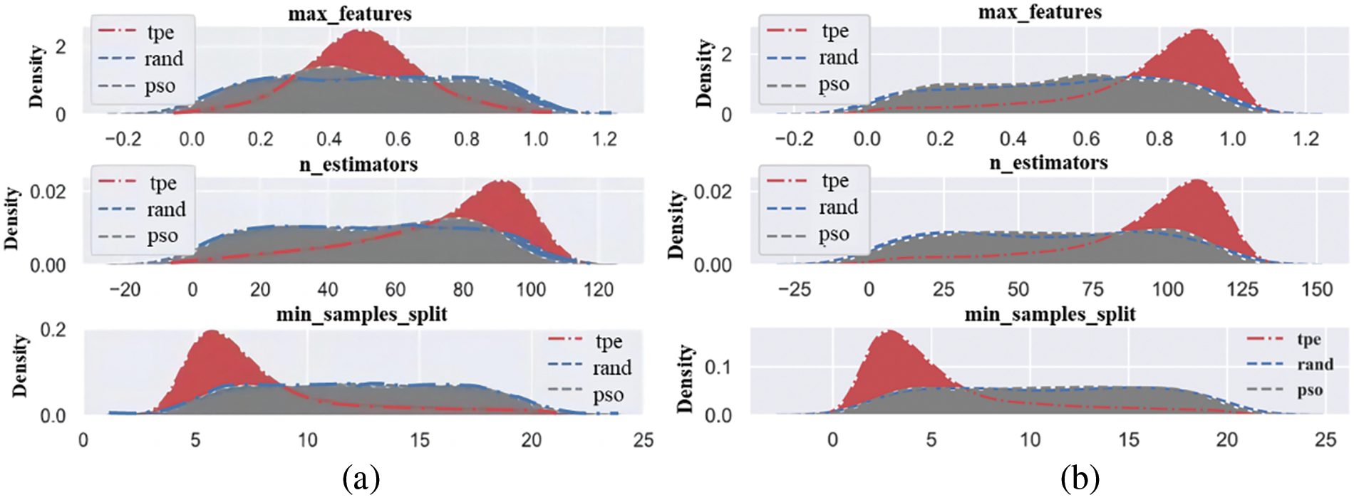
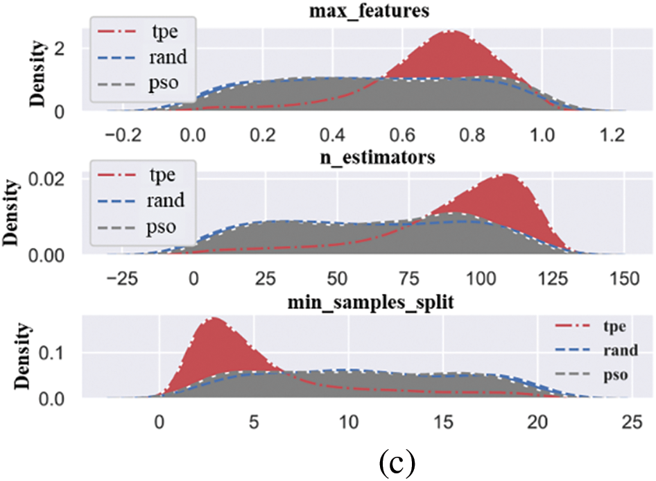
Figure 6: Hyper-parameter kernel density maps during optimization: (a) MCS data, (b) MTS data, and (c) BPF data

It can be observed that the BO method demonstrates distinct peaks in the selection of hyper-parameters, whereas the density distributions for the random search and PSO methods are more uniform. Specifically, the BO method exhibits a stronger tendency toward certain values in the three hyper-parameters, indicating its higher effectiveness in optimizing these parameters. Additionally, the average optimization times for the BO, PSO, and random search methods are 453, 211, and 319 s, respectively. Considering both optimization effectiveness and time cost, the BO and PSO methods have been chosen as the primary optimization techniques for the subsequent model refinement. The relationship between the loss value and each hyper-parameter in the iterative optimization process can be seen in Fig. 7.

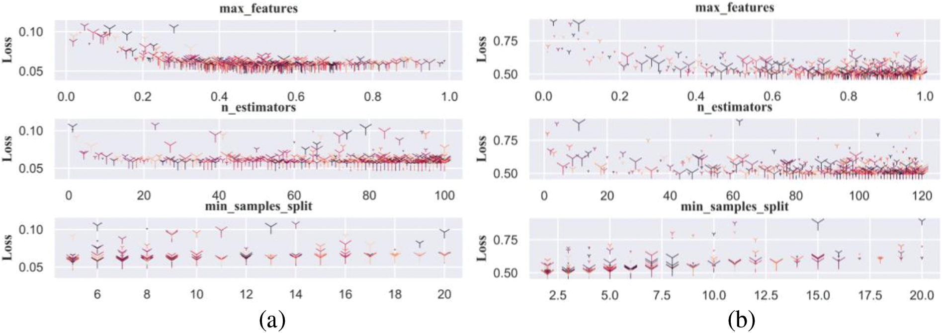
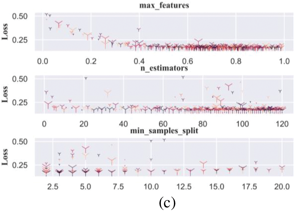
Figure 7: Relationship between parameter range and loss during optimization: (a) MCS data, (b) MTS data, and (c) BPF data

4.3 Comprehensive Analysis between Models

After optimizing the RF model using PSO and BO methods, we conducted a detailed comparative analysis of the performance of all models. Figs. 8–10 show the scatter distributions of the training and testing datasets for each regression model with MCS, MTS, and BPF as the predicted parameters, respectively. It can be seen that the optimized RF model outperforms the other models in all three prediction tasks. Whether on testing data or training data, its scatter distribution is very tight, demonstrating excellent predictive accuracy. The small performance discrepancy between the training and testing sets indicates that most models have strong generalization ability without over-fitting or under-fitting. The performance of XGBoost and SVR models is also good but slightly inferior to the optimized RF model in terms of predictive accuracy and consistency. KNN and DT models perform poorly across all three prediction tasks, with their scatter distributions being more dispersed and showing larger prediction errors.

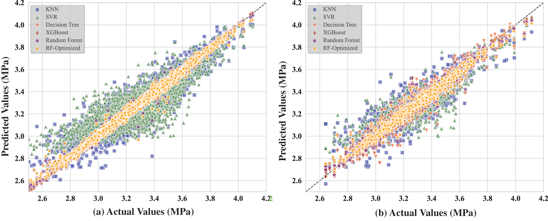
Figure 8: Comparison of predicted and measured values of each model for MCS: (a) testing data and (b) training data

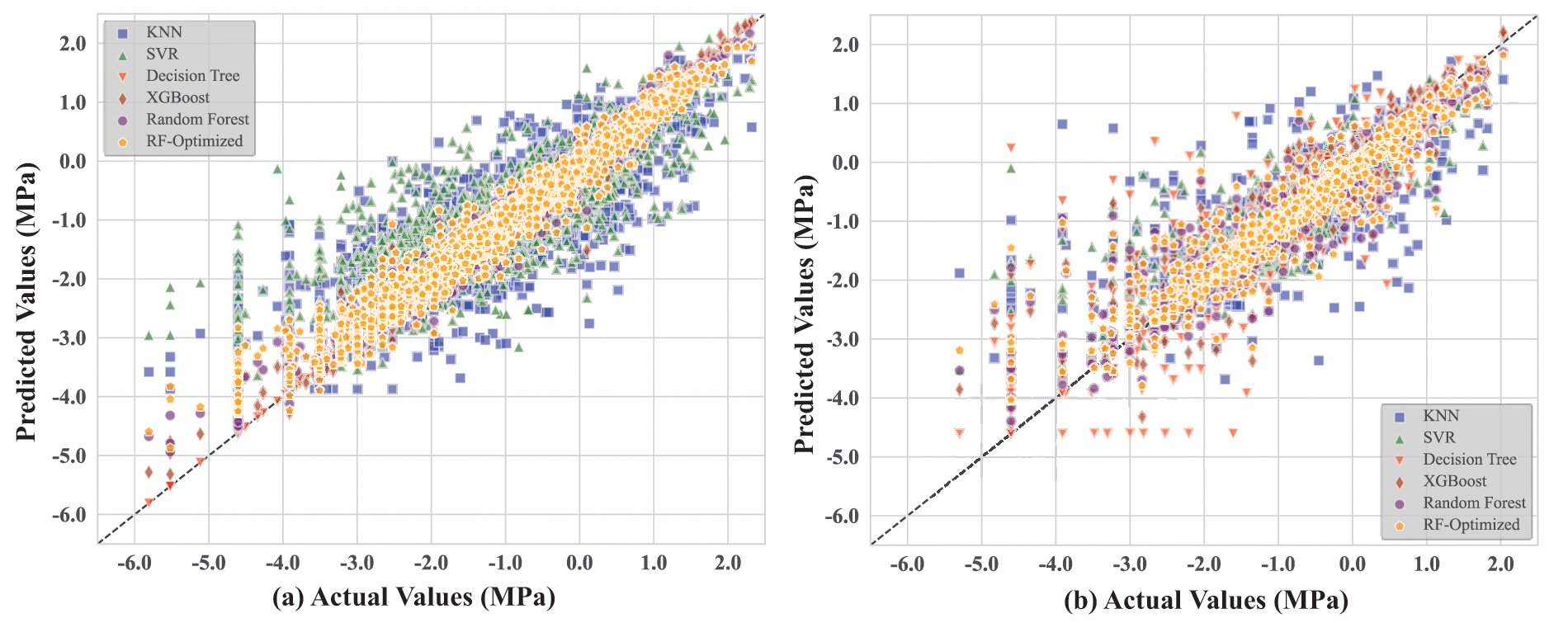
Figure 9: Comparison of predicted and measured values of each model for MTS: (a) testing data and (b) training data

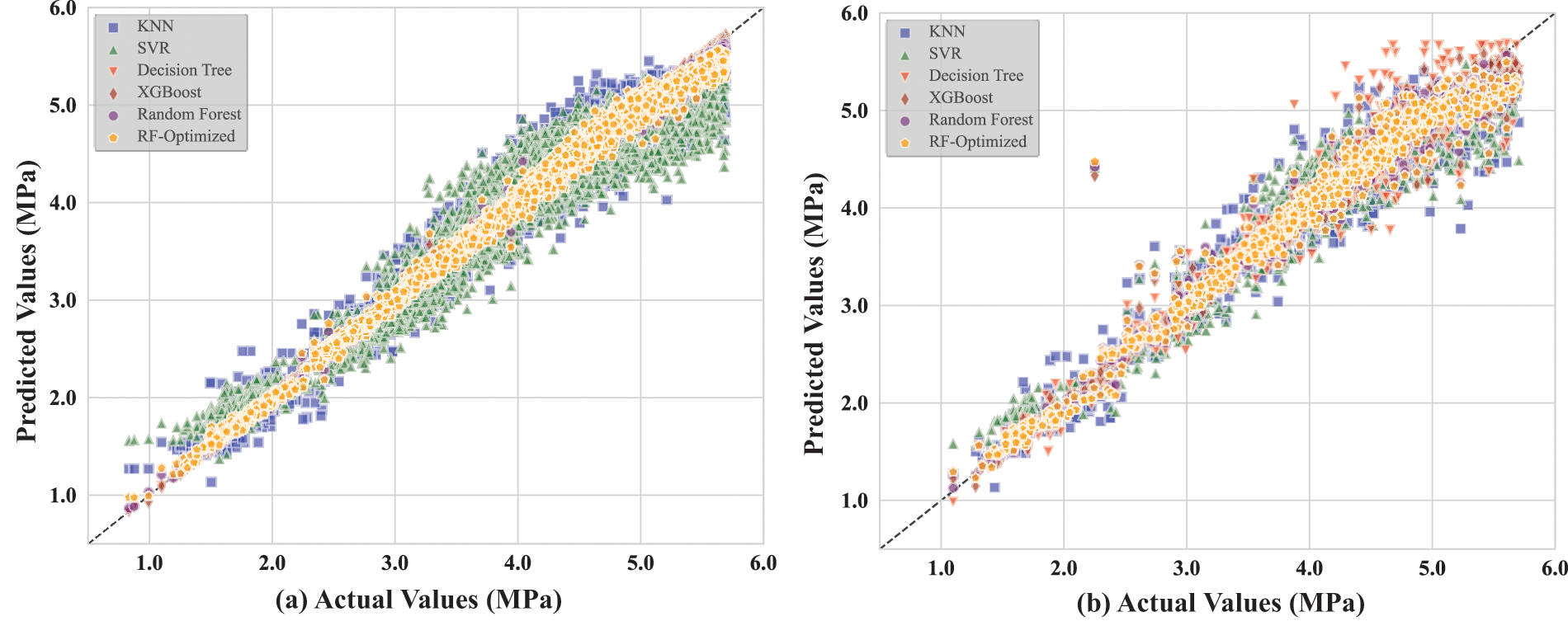
Figure 10: Comparison of predicted and measured values of each model for BPF: (a) testing data and (b) training data

Furthermore, combining the previous frequency distribution of the labels, the distribution of the model scatter should also be related to the distribution of the data itself. On account of the MCS data being roughly normally distributed, the fact is that its scatter plot data fits well. The MTS data is non-normally distributed, so its scatter distribution is not as tight as MCS. The comparison of the performance test results of each model is more intuitive and clearer in the bar chart presented in Fig. 11. Obviously, from different sub-sections of the results in Fig. 11, the optimized RF model is considered the optimal predictive technique in the predictions of MCS, MTS, and BPF.

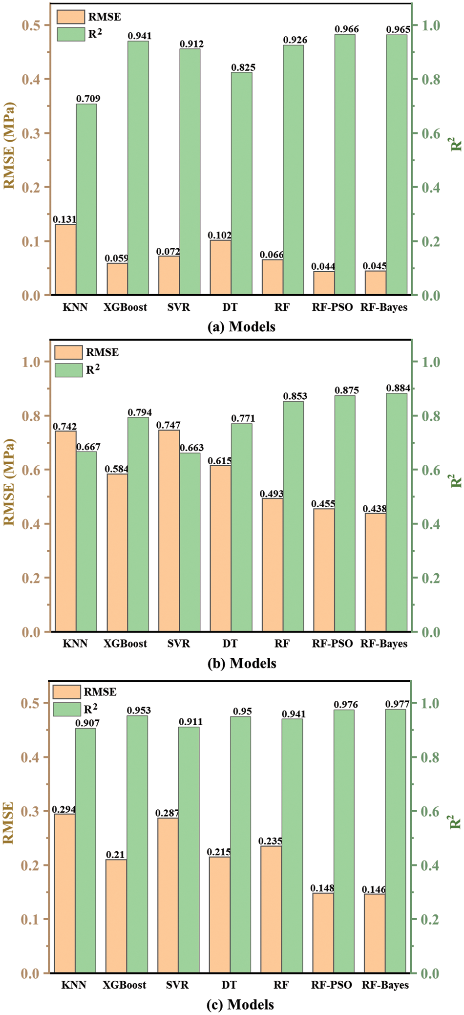
Figure 11: Evaluation indicators for each model: (a) MCS data, (b) MTS data, and (c) BPF data

4.4 Sensitivity and Uncertainty Analysis

Sobol sensitivity analysis is a global sensitivity analysis method used to quantitatively evaluate the influence of model input variables on output variables [58]. This method calculates the contribution of each input variable and its interactions with the model output by decomposing the variance of the output variable. The first-order sensitivity index measures the direct impact of a single input variable on the output variable, while the total sensitivity index measures the total contribution of an input variable to the output variable, including its interaction effects with other variables.

In this study, Sobol sensitivity analysis was used to evaluate the optimized models, and Fig. 12 shows the influence of each input variable on the prediction outputs for MCS, MTS, and BPF. In Fig. 12a, X16 and X17 exhibit significantly higher sensitivity indices, indicating that these two variables have the most substantial impact on MCS prediction. In Fig. 12b, the total sensitivity index is significantly higher than the first-order sensitivity index, indicating that MTS is influenced by the interactions between variables in the model. Among them, X13 and X17 are the most influential variables in the model. In Fig. 12c, X16, as the variable with the highest sensitivity index, is nearly close to 1, while the other variables are relatively low, indicating that X16 dominates the influence on BPF. Additionally, in the predictions of MCS, MTS, and BPF, X16 and X17, representing ultimate pile capacity and stroke, respectively, are the primary influencing variables, both direct effects and interactions with others variable.

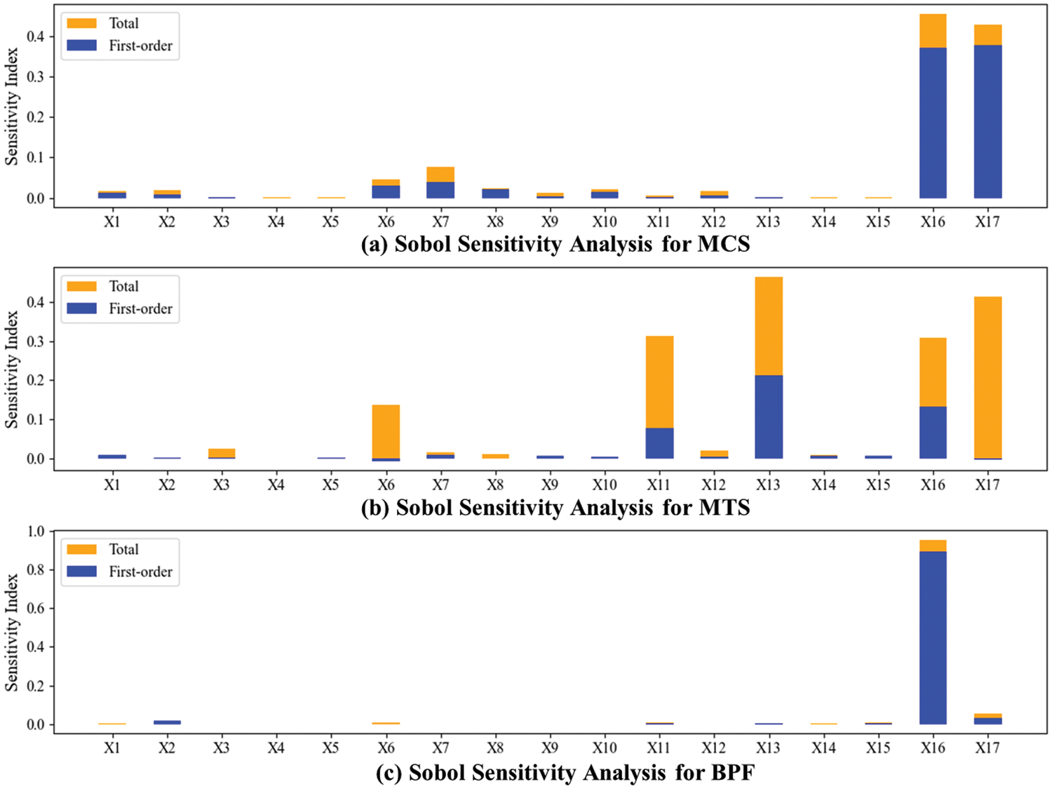
Figure 12: Sobol sensitivity analysis results for each model: (a) MCS, (b) MTS, and (c) BPF

Monte Carlo (MC) simulation is a numerical technique that uses random sampling for uncertainty analysis and risk assessment. By conducting numerous random samples and repeated experiments, MC simulation can generate distributions of variables, thereby quantifying the uncertainty in model predictions [59]. In this study, an optimized RF model was used for MC simulation to explain the model’s uncertainty. A total of 1000 simulations were conducted to ensure the robustness and reliability of the results.

Fig. 13 shows the comparison of the outputs for MCS, MTS, and BPF between the MC simulation and the optimized RF model. In the figure, the green represents the results generated by the MC simulation, and the orange represents the results produced by the optimized RF model. The distribution shapes of the optimized RF model’s predictions are very similar to those of the MC simulation results. This similarity indicates that the model’s performance under different input conditions aligns with the expected distribution, enhancing confidence in the model’s predictive reliability. Specifically, the median and interquartile range of the optimized RF model’s predictions are close to those of the MC simulation results, suggesting that both sets of predictions share similar central tendencies and degrees of dispersion. The similarity in the peak positions, widths, and shapes of the two results indicates that the model can capture the main characteristics of the input data and generate stable predictions, demonstrating good stability and reliability of the model.

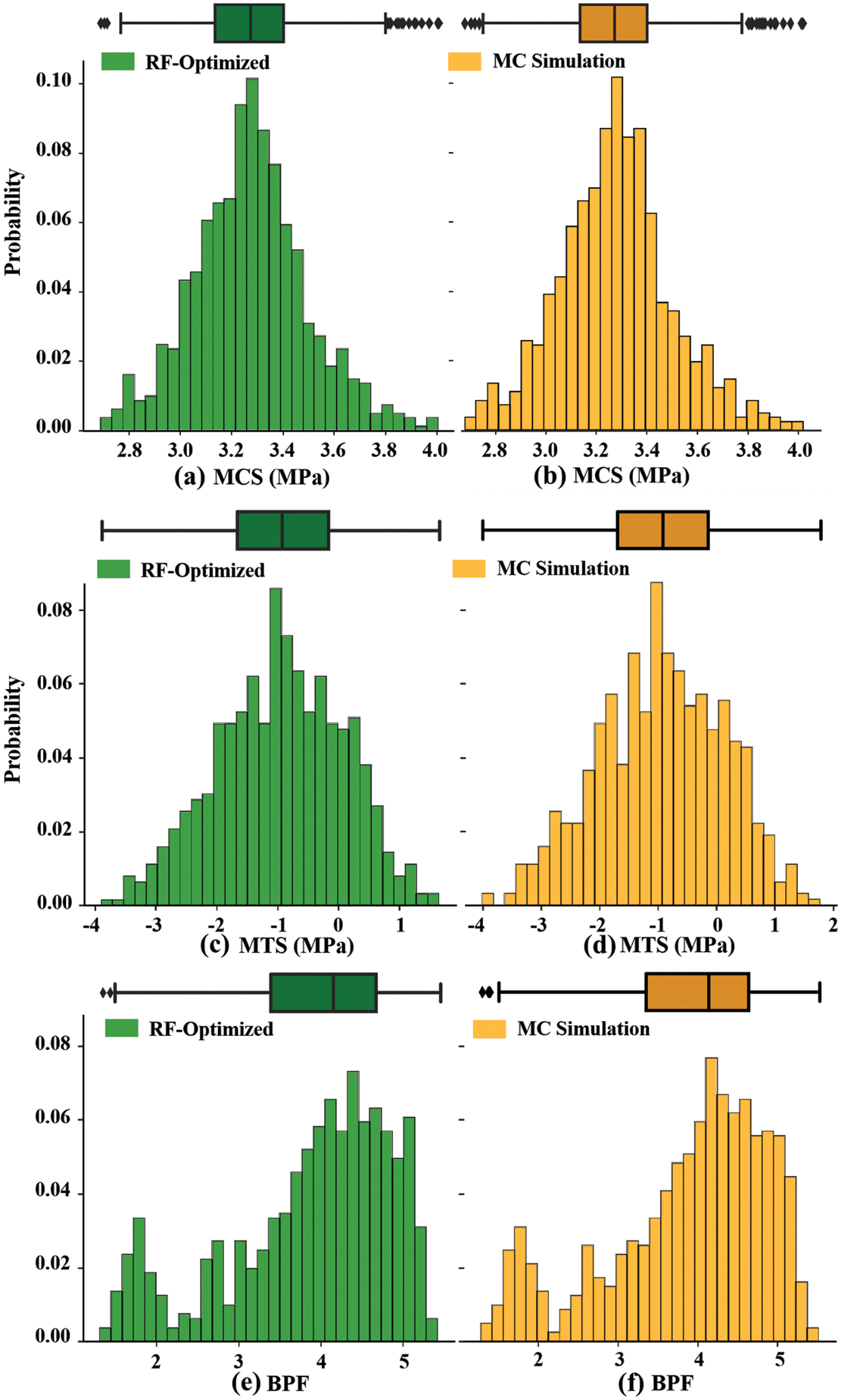
Figure 13: Distribution of prediction results before and after MC simulation, (a, c and e): training data; (b, d and f): testing data

4.5 Limitations and Future Research

Accurate prediction of pile drivability can effectively optimize pile design, achieving construction that is both safe and economical. In this study, we utilized BO and PSO to perform hyperparameter tuning on the RF model to evaluate and predict pile drivability. However, there are several limitations that need to be addressed in future research:

(1)   The optimized RF model significantly improves prediction accuracy and stability. However, as the dimensionality of the optimization search space increases, the computational complexity and resource consumption of BO increase significantly, while PSO tends to get trapped in local optima and is sensitive to parameter settings. Therefore, in practical applications, the specific characteristics of the problem should be considered comprehensively when selecting the most suitable optimization strategy, balancing the pros and cons of each method.

(2)   Future research can incorporate data from various engineering contexts, including different geological regions, soil types, and construction conditions, to provide a broader validation and prediction scope for the model. By introducing more diverse datasets, the predictive capability of the model will become more generalized, offering stronger support for pile drivability predictions under complex geological conditions.

(3)   To further enhance the performance and applicability of the model, future research can attempt to hybridize different optimization algorithms. By combining the strengths of various algorithms, the limitations of a single algorithm can be overcome. Additionally, new optimization algorithms, such as those based on deep learning or adaptive optimization, should be explored and developed to improve the model’s performance in high-dimensional spaces.

5  Conclusions

This study applied the RF machine learning model optimized by BO and PSO to predict the MCS, MTS, and BPF of the pile under various relevant factors. The established data set contains 4072 samples, of which 80% were used to train the models, and the remaining 20% were utilized to test the models. Then, the performance of the established RF was compared with the KNN, SVR, XGBoost, and DT models. In this study, RMSE and R2 were selected and calculated as two of the most popular performance indices in predictive models. It was found that the performance prediction of the optimized RF is higher than that of other implemented techniques. Meanwhile, it also proved that when the sample feature dimension is high, the RF model can still train the model effectively. It was shown that it has small generalization errors and strong generalization ability when solving such problems, and it can accurately reflect the complex relationship between piling and related parameters. In the test results, when predicting MCS, the RMSE and R2 of the optimal PF-PSO are 0.044 and 0.966, respectively. In predicting MTS, the RMSE and R2 of the optimal PF-Baye are 0.438 and 0.884, respectively. In predicting BPF, the RMSE and R2 of the optimal PF-Baye are 0.146 and 0.977, respectively. The above results showed that the RF optimization model using PSO and BO is an effective method to solve some complex engineering problems and can also provide a reference for other similar engineering problems in the future.

Acknowledgement: The authors thank the support of the National Science Foundation of China.

Funding Statement: This research was supported by the National Science Foundation of China (42107183).

Author Contributions: The authors confirm contribution to the paper as follows: study conception and design: Shengdong Cheng; data collection: Juncheng Gao; analysis and interpretation of results: Shengdong Cheng, Juncheng Gao, Hongning Qi; draft manuscript preparation: Shengdong Cheng, Hongning Qi. All authors reviewed the results and approved the final version of the manuscript.

Availability of Data and Materials: All data generated or analyzed during this study are included in this published article [51].

Conflicts of Interest: The authors declare that they have no conflicts of interest to report regarding the present study.

References

1. Xu J, Dai G, Gong W, Zhang Q, Haque A, Gamage RP. A review of research on the shaft resistance of rock-socketed piles. Acta Geotech. 2021;16(3):653–77. doi:10.1007/s11440-020-01051-2. [Google Scholar] [CrossRef]

2. Mohanty R, Suman S, Das SK. Prediction of vertical pile capacity of driven pile in cohesionless soil using artificial intelligence techniques. Int J Geotech Eng. 2018;12(2):209–16. doi:10.1080/19386362.2016.1269043. [Google Scholar] [CrossRef]

3. Suman S, Das SK, Mohanty R. Prediction of friction capacity of driven piles in clay using artificial intelligence techniques. Int J Geotech Eng. 2016;10(5):469–75. doi:10.1080/19386362.2016.1169009. [Google Scholar] [CrossRef]

4. Harandizadeh H, Jahed Armaghani D, Khari M. A new development of ANFIS-GMDH optimized by PSO to predict pile bearing capacity based on experimental datasets. Eng Comput. 2021;37(1):685–700. doi:10.1007/s00366-019-00849-3. [Google Scholar] [CrossRef]

5. Isaacs DV. Reinforced concrete pile formulae. J Instit Eng Australia. 1931;3(9):305–23. [Google Scholar]

6. Smith EAL. Pile-driving analysis by the wave equation. J Soil Mech Found Div. 1960;86(4):35–61. [Google Scholar]

7. Nath B. A continuum method of pile driving analysis: comparison with the wave equation method. Comput Geotech. 1990;10(4):265–85. [Google Scholar]

8. Zhang W, Goh AT. Multivariate adaptive regression splines and neural network models for prediction of pile drivability. Geosci Front. 2016;7(1):45–52. [Google Scholar]

9. Zhang W, Wu C, Li Y, Wang L, Samui P. Assessment of pile drivability using random forest regression and multivariate adaptive regression splines. Georisk: Asses Manag Risk for Eng Syst Geohazards. 2019;15(1):27–40. [Google Scholar]

10. Heidarie Golafzani S, Eslami A, Jamshidi Chenari R. Probabilistic assessment of model uncertainty for prediction of pile foundation bearing capacity; static analysis, SPT and CPT-based methods. Geotech Geol Eng. 2020;38(5):5023–41. [Google Scholar]

11. Chen Y, Yong W, Li C, Zhou J. Predicting the thickness of an excavation damaged zone around the roadway using the DA-RF hybrid model. Comput Model Eng & Sci. 2023;136(3):2507–26. doi:10.32604/cmes.2023.025714. [Google Scholar] [CrossRef]

12. Zhang W, Gu X, Hong L, Han L, Wang L. Comprehensive review of machine learning in geotechnical reliability analysis: algorithms, applications and further challenges. Appl Soft Comput. 2023;136(1):110066. [Google Scholar]

13. Qiu Y, Zhou J. Short-term rockburst prediction in underground project: insights from an explainable and interpretable ensemble learning model. Acta Geotech. 2023;18(12):6655–85. [Google Scholar]

14. Goh AT, Goh SH. Support vector machines: their use in geotechnical engineering as illustrated using seismic liquefaction data. Comput Geotech. 2007;34(5):410–21. [Google Scholar]

15. Asteris PG, Plevris V. Anisotropic masonry failure criterion using artificial neural networks. Neural Comput Appl. 2017;28(8):2207–29. [Google Scholar]

16. Asteris PG, Kolovos KG, Douvika MG, Roinos K. Prediction of self-compacting concrete strength using artificial neural networks. Eur J Environ Civil Eng. 2016;20(sup1):s102–22. doi:10.1080/19648189.2016.1246693. [Google Scholar] [CrossRef]

17. Asteris PG, Nikoo M. Artificial bee colony-based neural network for the prediction of the fundamental period of infilled frame structures. Neural Comput Appl. 2019;31(9):4837–47. doi:10.1007/s00521-018-03965-1. [Google Scholar] [CrossRef]

18. Luo J, Ren R, Guo K. The deformation monitoring of foundation pit by back propagation neural network and genetic algorithm and its application in geotechnical engineering. PLoS One. 2020;15(7):e0233398. doi:10.1371/journal.pone.0233398. [Google Scholar] [PubMed] [CrossRef]

19. Das SK, Basudhar PK. Undrained lateral load capacity of piles in clay using artificial neural network. Comput Geotech. 2006;33(8):454–9. doi:10.1016/j.compgeo.2006.08.006. [Google Scholar] [CrossRef]

20. Kordjazi A, Nejad FP, Jaksa MB. Prediction of ultimate axial load-carrying capacity of piles using a support vector machine based on CPT data. Comput Geotech. 2014;55(1):91–102. doi:10.1016/j.compgeo.2013.08.001. [Google Scholar] [CrossRef]

21. Zhang W, Goh AT, Zhang Y. Multivariate adaptive regression splines application for multivariate geotechnical problems with big data. Geotech Geol Eng. 2016;34(1):193–204. doi:10.1007/s10706-015-9938-9. [Google Scholar] [CrossRef]

22. Liu Q, Cao Y, Wang C. Prediction of ultimate axial load-carrying capacity for driven piles using machine learning methods. In: Proceedings of the 2019 IEEE 3rd Information Technology, Networking, Electronic and Automation Control Conference (ITNEC); 2019; Chengdu, China: IEEE. p. 334–340. [Google Scholar]

23. Huang L, Asteris PG, Koopialipoor M, Armaghani DJ, Tahir MM. Invasive weed optimization technique-based ANN to the prediction of rock tensile strength. Appl Sci. 2019;9(24):5372. doi:10.3390/app9245372. [Google Scholar] [CrossRef]

24. Qiu Y, Zhou J. Short-term rockburst damage assessment in burst-prone mines: an explainable XGBOOST hybrid model with SCSO algorithm. Rock Mech Rock Eng. 2023;56(12):8745–70. doi:10.1007/s00603-023-03522-w. [Google Scholar] [CrossRef]

25. Hajihassani M, Abdullah SS, Asteris PG, Armaghani DJ. A gene expression programming model for predicting tunnel convergence. Appl Sci. 2019;9(21):4650. doi:10.3390/app9214650. [Google Scholar] [CrossRef]

26. Zhang YL, Qin YG, Armaghsni DJ, Monjezi Ma, Zhou J. Enhancing rock fragmentation prediction in mining operations: A Hybrid GWO-RF model with SHAP interpretability. J Cent South Univ. 2024;31(6):1–14. doi:10.1007/s11771-024-5699-z. [Google Scholar] [CrossRef]

27. Breiman L. Bagging predictors. Mach Learn. 1996;24(2):123–40. [Google Scholar]

28. Breiman L. Random forests. Mach Learn. 2001;45(1):5–32. [Google Scholar]

29. Kuhn M, Johnson K. Applied predictive modeling. New York: Springer; 2013; vol. 26. [Google Scholar]

30. Rodriguez-Galiano V, Sanchez-Castillo M, Chica-Olmo M, Chica-Rivas MJOGR. Machine learning predictive models for mineral prospectivity: an evaluation of neural networks, random forest, regression trees and support vector machines. Ore Geol Rev. 2015;71(1):804–18. [Google Scholar]

31. Gislason PO, Benediktsson JA, Sveinsson JR. Random forests for land cover classification. Pattern Recognit Lett. 2006;27(4):294–300. [Google Scholar]

32. Dehghanbanadaki A, Khari M, Amiri ST, Armaghani DJ. Estimation of ultimate bearing capacity of driven piles in c-φ soil using MLP-GWO and ANFIS-GWO models: a comparative study. Soft Comput. 2021;25(5):4103–19. [Google Scholar]

33. Jong SC, Ong DEL, Oh E. State-of-the-art review of geotechnical-driven artificial intelligence techniques in underground soil-structure interaction. Tunnelling Undergr Space Technol. 2021;113(1):103946. doi:10.1016/j.tust.2021.103946. [Google Scholar] [CrossRef]

34. Kardani N, Zhou A, Nazem M, Shen SL. Estimation of bearing capacity of piles in cohesionless soil using optimised machine learning approaches. Geotech Geol Eng. 2020;38(2):2271–91. doi:10.1007/s10706-019-01085-8. [Google Scholar] [CrossRef]

35. Zhou J, Qiu Y, Khandelwal M, Zhu S, Zhang X. Developing a hybrid model of Jaya algorithm-based extreme gradient boosting machine to estimate blast-induced ground vibrations. Int J Rock Mech Min Sci. 2021;145(1):104856. doi:10.1016/j.ijrmms.2021.104856. [Google Scholar] [CrossRef]

36. Shi Y, Eberhart RC. Parameter selection in particle swarm optimization. In: Evolutionary Programming VII: Proceedings of the 7th International Conference; 1998 Mar 25–27; San Diego, CA, USA. Berlin: Springer. p. 591–600. [Google Scholar]

37. Li X, Yin M. A particle swarm inspired cuckoo search algorithm for real parameter optimization. Soft Comput. 2016;20(4):1389–1413. doi:10.1007/s00500-015-1594-8. [Google Scholar] [CrossRef]

38. Poli R, Kennedy J, Blackwell T. Particle swarm optimization an overview. Swarm Intell. 2007;1(1):33–57. doi:10.1007/s11721-007-0002-0. [Google Scholar] [CrossRef]

39. Jahed Armaghani D, Kumar D, Samui P, Hasanipanah M, Roy B. A novel approach for forecasting of ground vibrations resulting from blasting: modified particle swarm optimization coupled extreme learning machine. Eng Comput. 2021;37(4):3221–35. doi:10.1007/s00366-020-00997-x. [Google Scholar] [CrossRef]

40. Kennedy J, Eberhart R. Particle swarm optimization. In: IEEE International Conference on Neural Networks; 1995; Perth, Australia. p. 1942–8. [Google Scholar]

41. Zhou J, Qiu Y, Zhu S, Armaghani DJ, Li C, Nguyen H, Yagiz S. Optimization of support vector machine through the use of metaheuristic algorithms in forecasting TBM advance rate. Eng Appl Artif Intell. 2021;97(1):104015. doi:10.1016/j.engappai.2020.104015. [Google Scholar] [CrossRef]

42. Brits R, Engelbrecht AP, van den Bergh F. Locating multiple optima using particle swarm optimization. Appl Math Comput. 2007;189(2):1859–83. doi:10.1016/j.amc.2006.12.066. [Google Scholar] [CrossRef]

43. Zheng YL, Ma LH, Zhang LY, Qian JX. On the convergence analysis and parameter selection in particle swarm optimization. In: Proceedings of the 2003 International Conference on Machine Learning and Cybernetics (IEEE Cat. No. 03EX693); 2003 Nov; Xi’an, China: IEEE. p. 1802–7. [Google Scholar]

44. Mockus J, Tiesis V, Zilinskas A. The application of Bayesian methods for seeking the extremum. Towards Global Optim. 1978;2(117–129):2. [Google Scholar]

45. Garrido-Merchán EC, Hernández-Lobato D. Dealing with categorical and integer-valued variables in bayesian optimization with gaussian processes. Neurocomputing. 2020;380(4):20–35. doi:10.1016/j.neucom.2019.11.004. [Google Scholar] [CrossRef]

46. Han H, Jahed Armaghani D, Tarinejad R, Zhou J, Tahir MM. Random forest and bayesian network techniques for probabilistic prediction of flyrock induced by blasting in quarry sites. Nat Resour Res. 2020;29(2):655–67. doi:10.1007/s11053-019-09611-4. [Google Scholar] [CrossRef]

47. Qiu Y, Huang S, Armaghani DJ, Pradhan B, Zhou A, Zhou J. An optimized system of random forest model by global harmony search with generalized opposition-based learning for forecasting TBM advance rate. Comput Model Eng & Sci. 2024;138(3):2873–97. doi:10.32604/cmes.2023.029938. [Google Scholar] [PubMed] [CrossRef]

48. Qiu Y, Li C, Huang S, Ma D, Zhou J. An ensemble model of explainable soft computing for failure mode identification in reinforced concrete shear walls. J Build Eng. 2024;82(1):108386. doi:10.1016/j.jobe.2023.108386. [Google Scholar] [CrossRef]

49. Lizotte D. Practical bayesian optimization (Ph.D. Thesis). University of Alberta: Edmonton, Alberta; 2008. [Google Scholar]

50. Osborne MA, Garnett R, Roberts SJ. Gaussian processes for global optimization. In: 3rd International Conference on Learning and Intelligent Optimization (LION3); 2009; p. 1–15. [Google Scholar]

51. Jeon JK, Rahman MS. Fuzzy neural network models for geotechnical problems. In: Research project FHWA/NC/2006-52. Raleigh, NC, USA: North Carolina State University; 2008. [Google Scholar]

52. Zhang H, Zhou J, Armaghani DJ, Tahir MM, Pham BT, Huynh VV. A combination of feature selection and random forest techniques to solve a problem related to blast-induced ground vibration. Appl Sci. 2020;10(3):869. doi:10.3390/app10030869. [Google Scholar] [CrossRef]

53. Zhou J, Li E, Wei H, Li C, Qiao Q, Armaghani DJ. Random forests and cubist algorithms for predicting shear strengths of rockfill materials. Appl Sci. 2019;9(8):1621. doi:10.3390/app9081621. [Google Scholar] [CrossRef]

54. Zhou J, Qiu Y, Armaghani DJ, Zhang W, Li C, Zhu S, et al. Predicting TBM penetration rate in hard rock condition: a comparative study among six XGB-based metaheuristic techniques. Geosci Front. 2021;12(3):101091. [Google Scholar]

55. Zhou Y, Li S, Zhou C, Luo H. Intelligent approach based on random forest for safety risk prediction of deep foundation pit in subway stations. J Comput Civ Eng. 2019;33(1):05018004. [Google Scholar]

56. Amjad M, Ahmad I, Ahmad M, Wróblewski P, Kamiński P, Amjad U. Prediction of pile bearing capacity using XGBoost algorithm: modeling and performance evaluation. Appl Sci. 2022;12(4):2126. [Google Scholar]

57. Sun G, Hasanipanah M, Amnieh HB, Foong LK. Feasibility of indirect measurement of bearing capacity of driven piles based on a computational intelligence technique. Measurement. 2020;156:107577. [Google Scholar]

58. Zhang P. A novel feature selection method based on global sensitivity analysis with application in machine learning-based prediction model. Appl Soft Comput. 2019;85(1):105859. [Google Scholar]

59. Fang Y, Ma L, Yao Z, Li W, You S. Process optimization of biomass gasification with a Monte Carlo approach and random forest algorithm. Energy Convers Manag. 2022;264(1):115734. doi:10.1016/j.enconman.2022.115734. [Google Scholar] [CrossRef]