Incorporating Lasso Regression to Physics-Informed Neural Network for Inverse PDE Problem

1  Introduction

Dynamic systems are ubiquitous, and Partial Differential Equations (PDE) are the primary tools utilized to describe them. Examples include the Navier-Stokes equation for the motion of fluids, the Burgers’ equation for the propagation of waves, and the Schrödinger equation for the motion of microscopic particles [1–4]. Common PDE problems can be categorized into forward and inverse problems [5]. The forward problem refers to solving the PDE to obtain analytical or numerical solutions, allowing for a comprehensive system exploration. Traditionally, these problems are solved by numerical methods such as finite difference and finite element methods, which often entail heavy computational burdens [6]. However, the inverse problem aims to extract several governing PDEs to accurately describe a complex dynamic system based on abundant real experimental or operational data. Existing methods typically accomplish this by deriving from known physical principles like conservation laws or minimum energy principles, which often require substantial human resources and are hard to achieve [7].

Due to the rapid development of computer science and deep learning, Physics Informed Neural Networks (PINNs) have become widely applied in solving forward and inverse PDE problems [8,9]. Deep Neural Networks (DNN) are recognized for their powerful universal approximation capabilities and high expressivity, making them popular for solving PDE-related problems [10,11]. However, dealing with high-dimensional complex systems can not be exempt from the curse of dimensionality [7]. PINN integrates mathematical models, such as commonly known PDEs or boundary conditions, directly into the network architecture to address this issue. This is achieved by reinforcing the loss function with a residual term derived from the governing equation, which acts as a penalizing term, restricting the space of acceptable solutions and avoiding fitting DNN solely through the available data [12,13].

1.1 Related Work

The inverse PDE problems addressed in this work mainly focus on scenarios where abundant measure data is available for a specific dynamic system governed by some PDEs [14]. Without loss of generality, the PDE description can be formulated as follows:

ut=F[1,u,u2,⋯,∇u,∇2u,u⋅∇u⋯;λ](1)

where u=u(x,t) is the latent solution of the PDE; ut is the time derivate term; ∇ standards for gradient operation; F[⋅] is a complex nonlinear function composed of u and its derivate term and λ implies all known parameters.

The primary objective in inverse PDE problems can be regarded as to find the F[⋅] that optimally fits both the collected data and the physics laws [8,9]. An earlier idea on data-driven inverse PDE problem was to compare the experimental data’s numerical differentiations with analytic derivatives of candidate functions and apply the symbolic regression and the evolutionary algorithm to determine the nonlinear dynamical system [15,16]. Recently, Rudy et al. [17–19] shifted their focus towards sparse regression techniques. They used sparsity-promoting techniques by constructing an overcomplete dictionary comprising several simple functions and their derivatives, constituting the governing PDEs’ components. Thus, they proposed sequential threshold ridge regression (STRidge) to select candidates that most accurately represent the data.

However, these tasks still involve manually designing the differentiation operator and treating the whole process as conventional convex or nonconvex optimization, leading to representation errors. Raissi et al. [8] pioneered the concept of PINN, which embeds known physics law into deep neural networks to express PDEs. PINN can be seen as a universal nonlinear function approximator and excels in searching for nonlinear functions that satisfy the constraint conditions in the modeling process of PDEs by utilizing physics laws to constrain the training process and convergence of neural networks.

However, PINN still lags in accuracy and speed and struggles to handle the curse of dimensionality. In order to overcome these challenges, abundant works based on PINN have been undertaken [5,20–23]. Chen et al. [24] proposed a method for physics-informed learning of governing equations from limited data. It leverages pre-trained DNN with an Alternating Direction Optimization (ADO) algorithm. In this approach, DNN works as a surrogate model, while STRidge acts as the sparse selection algorithm. Long et al. [25,26] combined numerical approximation of differential operators by convolutions with a symbolic multi-layer neural network for model recovery to learn the underlying PDE model’s differential operators and the nonlinear response function. They also proved the feasibility of using convolutional neural networks as alternative models [25–28]. Rao et al. [29] proposed the Physics encoded Recurrent Convolutional Neural Network (PeRCNN), which performs convolutional operations on slices of collected data. They introduced the Pi-block for cascading convolution and recursive operations. In addition, they employed STRidge to implement PDE modeling and extended its application to various tasks. Huang et al. [30,31] treated data as robust principal components and outliers, optimizing the distribution of each part by convex optimization derivation and using STRidge as the sparse dictionary matching algorithm. Numerous methods nowadays continue to adopt the paradigm of combining PINN with sparse regression, particularly STRidge [32–36].

1.2 Our Method

STRidge plays a vital role in existing methods based on sparse dictionary regression. As proposed by Rudy et al. [17], STRidge combined the threshold least squares (STLS) and Ridge regression sequentially. STRidge can deal with the challenge of correlation in the data to some extent by substituting ridge regression for least squares in STLS. However, Ridge regression tends to retain the influence of all features rather than selecting some of them, especially when confronted with multiple related features. Hence, it still exhibits some shortcomings in dealing with high-dimensional multi-collinearity issues.

This study proposes Physics Informed Neural Network-Sequentially Threshold Least Squares-Lasso (PINN-STLasso), where Lasso Regression is incorporated into STLS. This new sparse regression module, STLasso, is integrated into the PINN framework to handle highly correlated data effectively. Using STLasso and PINN separately for sparse coefficients and DNN parameters, the governing equation of a dynamic system can be accurately determined by only a few observation data. The main contributions of the study are as follows:

(1) A novel module, STLasso, is proposed for sparse regression. The sparse coefficients, crucial for representing the discovered PDE, are computed through STLasso.

(2) A framework of PINN-STLasso is constructed. The sparse regression and DNN parameters are trained separately within the framework, improving the interpretability of the overall process.

(3) Experiments on canonical inverse PDE problems are conducted. The obtained results demonstrate that the proposed PINN-STLasso is superior to several recent relevant methods in terms of accuracy and efficiency.

The rest of this paper is organized as follows. Section 2 introduces the proposed STLasso and PINN-STLasso. Experiments on canonical inverse PDE problems are presented in Section 3 to demonstrate their performance. Finally, conclusions are drawn in Section 4.

2  The Proposed PINN-STLasso

2.1 STLasso

As described in Section 1, an effective solution to the inverse PDE problem often involves utilizing a well-constructed sparse dictionary Θ=[1,u,u2,⋯,∇u,∇2u,u⋅∇u⋯]. This study attempts to find a sparse coefficient Λ, such that

Residual:ut−ΘΛ→0(2)

With the help of the Universal Approximation theorem, a DNN can be employed to represent the latent solution u(θ) of PDEs, whose derivative is ut(θ). θ is adjustable parameters of the network. The constructed u(θ) and ut(θ) are required to simultaneously satisfy the results of collected measurements and adhere to known spares rules based on the thought of PINN. Thus, the loss function of the whole network is

Lloss=Lmeasurement+αLsparse+β‖Λ‖0(3)

where commonly

Lmeasurement=1Nm‖u(θ)−um‖22Lsaprse=1Ns‖ut(θ)−ΘΛ‖22(4)

α,β are weights of different loss, ‖⋅‖i(i=0,1,2) refers to li norm. Nm and Ns is the number of used data in each process.

Two kinds of parameters exist to be adjusted in this process: DNN parameters θ and sparse coefficient Λ. Generally, the optimization will be done individually, which means fixing one while training another. Common methods, such as ADO, recurrently adjust θ and Λ, resulting in a delay in training speed. On the other hand, noticing that norm is applied to ensure the sparsity of Λ, l0, but directly solving l0 norm is Non-deterministic Polynomial-hard (NP-hard) and unfixable. Generally, it uses convex relaxation-based techniques to transform the l0 norm minimization problem into an l1 norm minimization problem, such as l1 regularization. Then, the loss function of the sparse regression part will be

minΛ‖ut−ΘΛ‖22+‖Λ‖1(5)

It fits the traditional paradigm of Least Absolute Shrinkage and Selection Operator (Lasso) regression. Accordingly, this study proposes the STLasso module. The STLasso module is incorporated into the training process of DNN, using sparse regression without the need of recurrent optimization by integrating Lasso regression into STLS and forming a module. The detailed process of STLasso is depicted in Algorithm 1 and Algorithm 2.

2.2 PINN-STLasso

Inspired by literature [24], this study proposes the PINN-STLasso by integrating previously demonstrated STLasso into PINN. Fig. 1 depicts the schematic architecture of the entire network to solve an inverse PDE problem. In addition, unlike common methods that recurrently optimize θ and Λ, the proposed method can directly train two parameters separately. Specifically, our method focuses directly on reducing the loss (6).

L=1Nm‖u(θ)−um‖22+1Ns(‖ut(θ)−ΘΛ‖22+‖Λ‖1)(6)

Figure 1: Schematic architecture of the network

Fig. 2 illustrates the training process of the proposed PINN-STLasso. Treating STLasso as an independent module can be inserted into networks more flexibly. An additional Lasso regression operation Λ^:=lasso(Θ,ut;Λ^) is introduced between pretraining and formal training, which can accelerate the convergence of the DNN during formal training. Different colored blocks are utilized to denote their roles respectively, where brown ones operate on sparse coefficients Λ and those yellow corresponding to adjustments on the surrogate DNN model’s parameters θ. This network architecture provides a more precise visualization of the overall decision-making process, thereby improving the interpretability of the overall process.

Figure 2: Illustration of training process of PINN-STLasso

3  Experiments

This study conducted experiments on two canonical PDEs’ inverse problems, the Burgers equation and the Navier-Stocks equation, using scarce data. In addition, it applied the proposed method to experimental conditions to illustrate its effectiveness.

3.1 Burgers Equation

The Burgers equation is a nonlinear partial differential equation that simulates the propagation and reflection of shock waves, commonly found in simplified fluid mechanics, nonlinear acoustics, and gas dynamics, whose general form can be expressed as follows (7):

ut=−uux+νuxx(7)

where u is flow velocity; x and t corresponding to spatial and temporal dimension; ν is the diffusion coefficient, which is 0.1 in this experiment. In this experiment, the data is extracted from the open dataset of the literature [17], which u is discretized into 256 spatial grid points for 101-time steps with a Gaussian initial condition, forming a data size of R256×101. Specifically, 10 points are randomly selected to simulate ten randomly placed sensors. They are used for DNN training, and 50,000 collection points are generated by Latin hypercube sampling for sparse regression, which is only 3.19% of the data used in the literature [17]. Based on the aforementioned experimental requirements, 16 candidate functions Θ∈R16×1 are utilized to reconstruct the PDE, consisting of polynomial terms, derivatives, and their multiplication. Thus, the constructed sparse dictionary will be Θ={1,u,u2,u3,ux,uux,u2ux,u3ux,⋯,u3uxxx}. The setting of the sparse dictionary can be very flexible, to some extent, depending on prior knowledge and experience. 10% random noise is added to the data to simulate actual measurement errors. During the training process, the network went through 10,000 times Limited-memory Broyden–Fletcher–Goldfarb–Shanno (L-BFGS-B) Pretraining. In formal training, the ADO process takes ten iterations for sparse regression and 1000 times optimization with Adam in each epoch.

Table 1 presents a comparison of the proposed PINN-STLasso with several recent methods for inverse PDE problems in terms of reconstruction error, including Physics Informed Neural Network-Sparse Regression (PINN-SR) [24], Partial Differential Equation-Find (PDE-Find) [17]. As the proposed method can handle sparse data, whereas other methods can fail under similar conditions, the error values are directly extracted from corresponding studies. Nonetheless, the proposed PINN-STLasso outperforms other methods, even with less data. All errors are computed by Eq. (8).

η=‖Λ^−Λ‖2‖Λ‖2(8)

where Λ^ and Λ stands for detected value and ground truth. Fig. 3 compares the reconstructed Burgers equation with the ground truth.

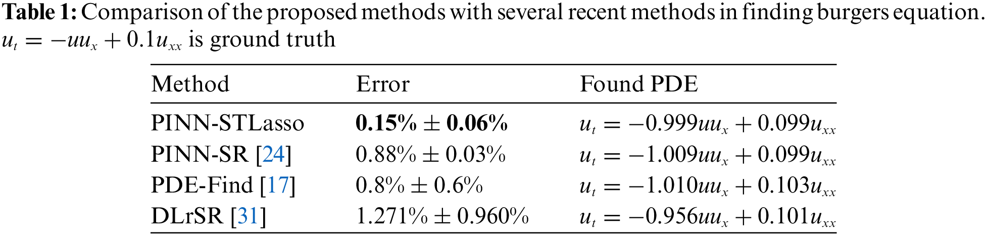
Figure 3: Comparison of predicted burgers equation with ground truth

3.2 Navier-Stocks Equation

Navier-Stokes (NS) equations are commonly employed to describe the motion equation of momentum conservation in viscous incompressible fluids. The NS equation can determine the fluid flow with certain initial and boundary conditions. In this study, the NS equation is utilized to model a 2D fluid flow passing a circular cylinder with the local rotation dynamics, as shown in Fig. 4, where partial data used in the modeling process is highlighted by a red box, whose general form is

wt=−(u⋅∇)w+v∇2w(9)

where w is the spatiotemporally variant vorticity; u={ux,uy} is the velocity of the fluid in two dimensions; ν is the kinematic viscosity, which is 0.01 in this experiment. Similar to Burgers’ equation, 500 points, consisting of {ux,uy,w} and 60 times steps’ records, are randomly selected to simulate randomly placed sensors. They are used for DNN training with 60,000 collection points generated by Latin hypercube sampling for sparse regression, which is only 10% of data used in [17]. The size of the protentional sparse library is Θ∈R60×1, in the form of Θ={1,ωx,ωy,ωxx,ωyy,uωx,vωx,ωωx,⋯,u2ωx,v2ωx,ω2ωx}, consisting of polynomial terms, derivatives, and their multiplication. 10% random noise is also added. During the training process, the network has gone through 5000 times pretraining with Adam optimizer and 10,000 times L-BFGS-B Pretraining. In formal training, the ADO process takes ten iterations for sparse regression and 1000 times optimization with Adam in each epoch. 20,000 Adam optimizations were used in the post-training phase.

Figure 4: Dynamic model used in this work

Table 2 shows a comparison of several methods in NS equation reconstruction problems. PDE-Find fails to get a result in the 10% noise condition. Therefore, the presented result is in 1% noise condition. Despite using less data, the proposed PINN-STLasso still outperforms other methods in complex problems. Fig. 5 compares the predicted Navier-Stokes equation with the ground truth at a specific time.

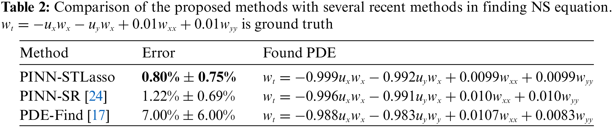
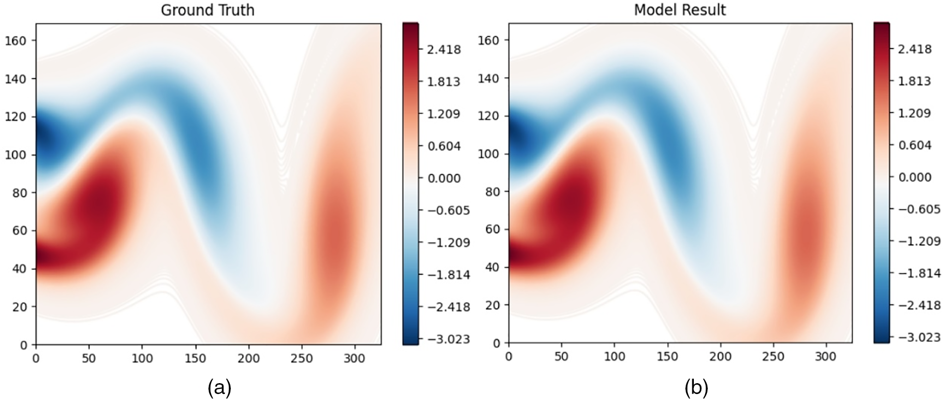
Figure 5: Comparison of predicted Navier-Stokes equation with ground truth in a specific time: (a) Ground truth of Navier-Stokes equation (b) Model prediction result of Navier-Stokes equation

3.3 Experimental Reaction-Diffusion Equation

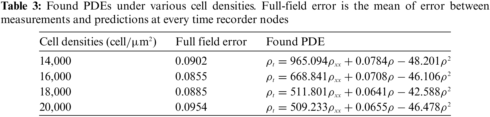
This study conducts an experiment to discover the governing equation of a cell migration and proliferation process to demonstrate the performance of the proposed STLasso on complicated systems and actual experimental situations. The data used in the experiment is collected from vitro cell migration (scratch) assays, which remain sparse and noisy. With cells distributed in wells as uniformly as possible, results for initial cell densities of 14,000, 16,000, 18,000, and 20,000 cells per well are collected. After seeding, cells are grown overnight for attachment and some growth. To quantify the cell density profile, in each record node, images captured by high-precision cameras are uniformly divided with a width of 50 μm, from which manual cell counting is employed to estimate the cell density at positions x=25,75,125,⋯,1925 µm∈R1x38. After seeding, cells are grown overnight for attachment and some growth. Images of the collective cell spreading are recorded every two hours for 48 h. This research will use cell density distributions at different time instants, specifically, 12, 24, 36, and 48 h after seeding. Three identically prepared experiments are replicated for each cell density, and their mean is considered the final result. The specified description of the experimental data can be found in the literature [37].

This study aims to discover PDEs that can describe the changes in cell concentration under different cell densities. Based on known prior knowledge, the process of cell migration and proliferation can be viewed as a typical Reaction-Diffusion process with migration as cell reaction and proliferation as growing diffusion. Thus, we assume that the PDEs describing this process hold the general form of Eq. (10).

ρt=γρxx+F(ρ)(10)

where ρ is cell density; γ is aiming diffusion coefficient to be found; F(ρ) is underlying nonlinear reaction function.

Similar to the previous experimental design, a sparse dictionary with nine candidate function terms {1,ρ,ρ2,ρ3,ρx,ρxx,ρρx,ρ2ρx,ρ3ρxx} is established to perform coefficient regression. Table 3 lists the results of all cell densities that were discovered. These results follow the Reaction-Diffusion (RD) equation form ρt=γρxx+αρ+βρ2, which conforms to the Fisher-Kolmogorov model preset [37].

The measurements and prediction in different time nodes (12, 24, 36, and 48 h) are depicted as shown in Fig. 6a–d to more intuitively demonstrate the relationship between the discovered equations and measured values. Prediction is derived for each found PDE considering the measurement at0 h initial and ρx(x=0,t)=ρx(x=1900,t)=0 a boundary condition. In each individual experiment, only 38 pieces of measurement were used, which is extremely scarce and can fail for most other methods. Experimental results showed that the proposed PINN-STLasso can successfully discover equations and demonstrate relatively high accuracy.

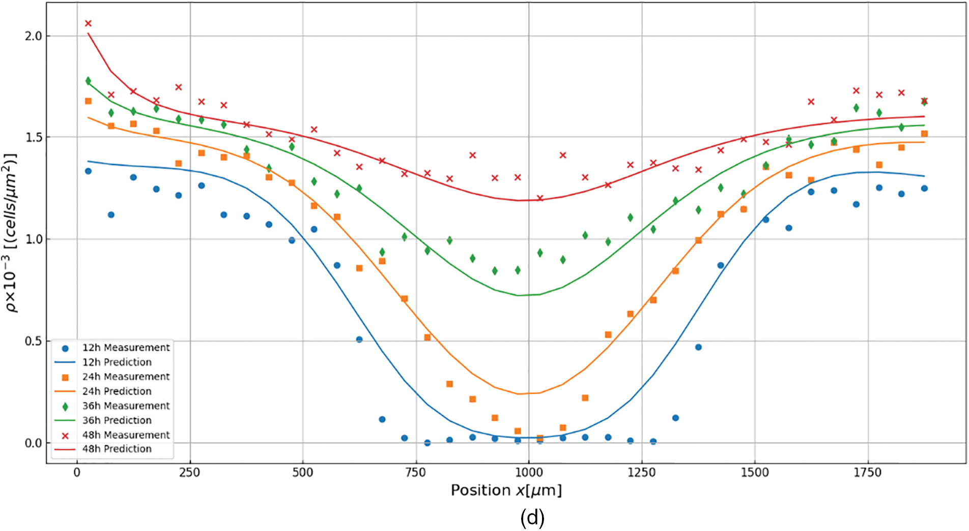
Figure 6: Discovery results for cell migration and proliferation under different cell densities, (a) 14,000 cells per well; (b) 16,000 cells per well; (c) 18,000 cells per well; (d) 20,000 cells per well. In all figures, dots represent measurement, and lines depict prediction

3.4 Discussion

This study conducts experiments on several canonical inverse PDE problems and real experimental conditions. Results and comparison indicated that the proposed PINN-STLasso outperforms existing methods in the following aspects:

1) Based on the idea of calculating equation coefficients through the sparse regression method STLasso, which introduces known physical prior knowledge into the computational process. Specifically, in PINN-STLasso, the training of surrogate models and the formation of the sparse dictionaries are guided by physical priors, significantly reducing the demand for training data and enhancing the robustness of data noise in this method.

2) The sparse regression and DNN parameters are trained by different network parts, improving the overall process’s interpretability. Unlike most common methods based solely on deep networks, PINN-STLasso takes DNN, specifically, Multi-layer Perceptron, as a surrogate model. With the help of the universal approximate rule, the role of surrogate DNN can be interpreted as a nonlinear approximation of the original solution. In contrast, Lasso sparse computing is a clear iterative solution process with a completely transparent calculation principle and process. Accordingly, the proposed PINN-STLasso is very superior in terms of interpretability.

4  Conclusion

This research proposes PINN-STLasso, a method incorporating Lasso Regression into Physics-Informed Neural Networks for solving Inverse PDE problems. A sparse regression module, STLasso, is established for optimizing sparse parameters by combining Lasso and STLS. STLasso is then inserted into PINN to identify PDE expressions from observations. Experiments conducted on canonical PDE systems demonstrate that the proposed PINN-STLasso outperforms several recent methods regarding prediction accuracy.

However, there still exist several challenges in this research to be further explored: Lasso regression cannot address problems in complex domains, such as the Schrödinger equation, requiring the development of specialized methods; for highly complicated problems, such as the Reaction-Diffusion process, the DNN-based method still performs poorly, necessitating further exploration of related issues.

Acknowledgement: The authors acknowledge the support from the National Key Lab of Aerospace Power System and Plasma Technology of Xi’an Jiaotong University, China. We are also thankful for the insightful comments from anonymous reviewers, which have greatly improved this manuscript.

Funding Statement: The authors received no specific funding for this study.

Author Contributions: Study conception and design: Meng Ma, Liu Fu; data collection: Meng Ma, Liu Fu; analysis and interpretation of results: Meng Ma, Liu Fu, Xu Guo, Zhi Zhai; draft manuscript preparation: Meng Ma, Liu Fu, Xu Guo. All authors reviewed the results and approved the final version of the manuscript.

Availability of Data and Materials: Data will be made available on request.

Ethics Approval: Not applicable.

Conflicts of Interest: The authors declare that they have no conflicts of interest to report regarding the present study.

References

1. Bleecker D. Basic partial differential equations. Boca Raton, FL, USA: Chapman and Hall/CRC; 2018. [Google Scholar]

2. Renardy M, Rogers RC. An introduction to partial differential equations. Midtown Manhattan, New York City, USA: Springer Science & Business Media; 2006. [Google Scholar]

3. Evans LC. Partial differential equations. Providence, Rhode Island, USA: American Mathematical Society; 2022. [Google Scholar]

4. Wandel N, Weinmann M, Klein R. Learning incompressible fluid dynamics from scratch—towards fast, differentiable fluid models that generalize. arxiv Preprint arxiv:2006.08762. 2020. [Google Scholar]

5. Yuan L, Ni Y, Deng X, Hao S. A-PINN: auxiliary physics informed neural networks for forward and inverse problems of nonlinear integro-differential equations. J Comput Phys. 2022;462:111260. doi:10.1016/j.jcp.2022.111260. [Google Scholar] [CrossRef]

6. Ames WF. Numerical methods for partial differential equations. Cambridge, MA, USA: Academic press; 2014. [Google Scholar]

7. Cuomo S, Di Cola VS, Giampaolo F, Rozza G, Raissi M, Piccialli F. Scientific machine learning through physics–informed neural networks: where we are and what’s next. J Sci Comput. 2022;92(3):88. doi:10.1007/s10915-022-01939-z. [Google Scholar] [CrossRef]

8. Raissi M, Perdikaris P, Karniadakis GE. Physics-informed neural networks: a deep learning framework for solving forward and inverse problems involving nonlinear partial differential equations. J Comput Phys. 2019;378:686–707. doi:10.1016/j.jcp.2018.10.045. [Google Scholar] [CrossRef]

9. Cai S, Mao Z, Wang Z, Yin M, Karniadakis GE. Physics-informed neural networks (PINNs) for fluid mechanics: a review. Acta Mech Sin. 2021;37(12):1727–38. doi:10.1007/s10409-021-01148-1. [Google Scholar] [CrossRef]

10. Jiang X, Wang X, Wen Z, Li E, Wang H. Practical uncertainty quantification for space-dependent inverse heat conduction problem via ensemble physics-informed neural networks. Int Commun Heat Mass Transf. 2023;147(2):106940. doi:10.1016/j.icheatmasstransfer.2023.106940. [Google Scholar] [CrossRef]

11. Wen Z, Li Y, Wang H, Peng Y. Data-driven spatiotemporal modeling for structural dynamics on irregular domains by stochastic dependency neural estimation. Comput Methods Appl Mech Eng. 2023;404:115831. doi:10.1016/j.cma.2022.115831. [Google Scholar] [CrossRef]

12. Zhang Z, Cai S, Zhang H. A symmetry group based supervised learning method for solving partial differential equations. Comput Methods Appl Mech Eng. 2023;414(5):116181. doi:10.1016/j.cma.2023.116181. [Google Scholar] [CrossRef]

13. Zhang Z, Zhang H, Zhang L, Guo L. Enforcing continuous symmetries in physics-informed neural network for solving forward and inverse problems of partial differential equations. J Comput Phys. 2023;492(153):112415. doi:10.1016/j.jcp.2023.112415. [Google Scholar] [CrossRef]

14. Isakov V. Inverse problems for partial differential equations. Midtown Manhattan, New York, NY, USA: Springer; 2006. [Google Scholar]

15. Bongard J, Lipson H. Automated reverse engineering of nonlinear dynamical systems. Proc Nat Acad Sci. 2007;104(24):9943–48. doi:10.1073/pnas.0609476104. [Google Scholar] [PubMed] [CrossRef]

16. Schmidt M, Lipson H. Distilling free-form natural laws from experimental data. Science. 2009;324(5923):81–5. doi:10.1126/science.1165893. [Google Scholar] [PubMed] [CrossRef]

17. Rudy SH, Brunton SL, Proctor JL, Kutz JN. Data-driven discovery of partial differential equations. Sci Adv. 2017;3(4):e1602614. doi:10.1126/sciadv.1602614. [Google Scholar] [PubMed] [CrossRef]

18. Schaeffer H. Learning partial differential equations via data discovery and sparse optimization. Proc Royal Soc A: Math, Phy Eng Sci. 2017;473(2197):20160446. doi:10.1098/rspa.2016.0446. [Google Scholar] [PubMed] [CrossRef]

19. Brunton SL, Proctor JL, Kutz JN. Discovering governing equations from data by sparse identification of nonlinear dynamical systems. Proc Nat Acad Sci. 2016;113(15):3932–37. doi:10.1073/pnas.1517384113. [Google Scholar] [PubMed] [CrossRef]

20. Zheng J, Yang Y. M-WDRNNs: mixed-weighted deep residual neural networks for forward and inverse PDE problems. Axioms. 2023;12(8):750. doi:10.3390/axioms12080750. [Google Scholar] [CrossRef]

21. Lemhadri I, Ruan F, Tibshirani R. LassoNet: neural networks with feature sparsity. In: Proceedings of The 24th International Conference on Artificial Intelligence and Statistics, 2021; PMLR; vol. 130, p. 10–8. [Google Scholar]

22. Lu L, Meng X, Mao Z, Karniadakis GE. DeepXDE: a deep learning library for solving differential equations. Siam Rev Soc Ind Appl Math. 2021;63(1):208–28. doi:10.1137/19M1274067 2021/01/01. [Google Scholar] [CrossRef]

23. Yang M, Foster JT. Multi-output physics-informed neural networks for forward and inverse PDE problems with uncertainties. Comput Methods Appl Mech Eng. 2022;402(1):115041. doi:10.1016/j.cma.2022.115041. [Google Scholar] [CrossRef]

24. Chen Z, Liu Y, Sun H. Physics-informed learning of governing equations from scarce data. Nat Commun. 2021;12(1):6136. doi:10.1038/s41467-021-26434-1. [Google Scholar] [PubMed] [CrossRef]

25. Long Z, Lu Y, Ma X, Dong B. PDE-Net: learning PDEs from data. In: Proceedings of the 35th International Conference on Machine Learning, 2018; PMLR; vol. 80, p. 3208–16. [Google Scholar]

26. Long Z, Lu Y, Dong B. PDE-Net 2.0: learning pdes from data with a numeric-symbolic hybrid deep network. J Comput Phys. 2019;399(24):108925. doi:10.1016/j.jcp.2019.108925. [Google Scholar] [CrossRef]

27. Dong B, Jiang Q, Shen Z. Image restoration: wavelet frame shrinkage, nonlinear evolution PDEs, and beyond. Multiscale Model Simul. 2017;15(1):606–60. doi:10.1137/15M1037457. [Google Scholar] [CrossRef]

28. Cai J, Dong B, Osher S, Shen Z. Image restoration: total variation, wavelet frames, and beyond. J Am Math Soc. 2012;25(4):1033–89. doi:10.1090/S0894-0347-2012-00740-1. [Google Scholar] [CrossRef]

29. Rao C, Ren P, Wang Q, Buyukozturk O, Sun H, Liu Y. Encoding physics to learn reaction-diffusion processes. Nat Mach Intell. 2023;5(7):765–79. doi:10.1038/s42256-023-00685-7. [Google Scholar] [CrossRef]

30. Huang K, Tao S, Wu D, Yang C, Gui W. Physical informed sparse learning for robust modeling of distributed parameter system and its industrial applications. IEEE Trans Autom Sci Eng. 2023. doi:10.1109/TASE.2023.3298806. [Google Scholar] [CrossRef]

31. Li J, Sun G, Zhao G, Lehman LWH, editors. Robust low-rank discovery of data-driven partial differential equations. Proc AAAI Conf Artif Intell. 2020;34(1):767–74. doi:10.1609/aaai.v34i01.5420. [Google Scholar] [CrossRef]

32. Yu J, Lu L, Meng X, Karniadakis GE. Gradient-enhanced physics-informed neural networks for forward and inverse PDE problems. Comput Methods Appl Mech Eng. 2022;393(6):114823. doi:10.1016/j.cma.2022.114823. [Google Scholar] [CrossRef]

33. Yang L, Meng X, Karniadakis GE. B-PINNs: bayesian physics-informed neural networks for forward and inverse PDE problems with noisy data. J Comput Phys. 2021;425:109913. doi:10.1016/j.jcp.2020.109913. [Google Scholar] [CrossRef]

34. Pakravan S, Mistani PA, Aragon-Calvo MA, Gibou F. Solving inverse-PDE problems with physics-aware neural networks. J Comput Phys. 2021;440(4):110414. doi:10.1016/j.jcp.2021.110414. [Google Scholar] [CrossRef]

35. Smets BMN, Portegies J, Bekkers EJ, Duits R. PDE-based group equivariant convolutional neural networks. J Math Imaging Vis. 2023;65(1):209–39. doi:10.1007/s10851-022-01114-x. [Google Scholar] [CrossRef]

36. Hess P, Drüke M, Petri S, Strnad FM, Boers N. Physically constrained generative adversarial networks for improving precipitation fields from earth system models. Nat Mach Intell. 2022;4(10):828–39. doi:10.1038/s42256-022-00540-1. [Google Scholar] [CrossRef]

37. Jin W, Shah ET, Penington CJ, McCue SW, Chopin LK, Simpson MJ. Reproducibility of scratch assays is affected by the initial degree of confluence: experiments, modelling and model selection. J Theor Biol. 2016;390:136–45. doi:10.1016/j.jtbi.2015.10.040. [Google Scholar] [PubMed] [CrossRef]