A Pooling Method Developed for Use in Convolutional Neural Networks

1  Introduction

Artificial intelligence has brought many different applications and innovations to today’s technology field [1–3]. Artificial intelligence is seen as an area open to development as it has great potential in many different areas [4–6]. Therefore, new applications and algorithms are constantly being developed with artificial intelligence [7–9]. Artificial intelligence covers a wide range of disciplines and includes different capabilities and application areas. These disciplines enable algorithms to analyze data to recognize data and predict future events [10,11], to identify and represent complex patterns using multilayer artificial neural networks [12,13], and to enable computers to process and understand visual data [14,15].

In recent years, artificial intelligence-based deep learning algorithms consisting of multi-layered model structures have been developed to learn complex data efficiently [16,17]. These algorithms are used in many areas such as object classification, object recognition, and object detection. Many different neural network architectures are used in deep learning for different types of data and applications [18–20]. Convolutional neural networks, one of these neural network architectures and the most preferred in deep learning methods are very effective in tasks such as analysis, recognition, and classification of images [21–24]. Convolutional neural networks (CNNs) are specifically optimized for detecting and representing objects in images [21]. CNN are deep learning architectures widely used on pre-processed data types. These networks are designed to recognize local structures of input data, unlike traditional artificial neural networks. CNNs consist of convolution layers, pooling layers, activation functions, and fully connected layers [25–29].

Pooling layers, one of the important components of CNN, are layers that are usually added between layers and enable the neural network to run faster by reducing the data size, number of parameters, and amount of memory of the neural network. Pooling layers are used to reduce the feature map of the previous layer. Thus, increasing the scalability of the network and reducing the computational cost [30–32]. While pooling layers help prevent the loss of local features during the learning process of the network, they can also increase the network’s resilience to translation and scale changes to a certain extent. This enables CNNs to be effective in many application areas, such as visual recognition. Therefore, pooling layers are considered an important component that improves the efficiency of convolutional neural networks. Pooling is usually done using different techniques such as maximum pooling, average pooling, or minimum pooling [33–37].

Maximum pooling works by taking the maximum value of pixels within a given image size. In convolutional neural networks, it helps preserve the most salient features while reducing the size of the feature map. It is also considered an important component in improving performance in CNNs and the overall efficiency of the network by reducing the computational cost of the network and the risk of overfitting [32,38]. However, maximum pooling has many disadvantages, such as the fact that it selects only the most prominent feature from each region, causing other important features to be lost and causing information loss, finer details being neglected while emphasizing salient features in the feature map, and a certain amount of information loss occurring when pooling layers are used sequentially [37,39–42].

Average pooling works by taking the average value of pixels within a given image size. Salient features of the feature map, such as maximum pooling, are only effective in reducing noise in images and providing smoother transitions, without emphasis. Therefore, it is preferred in certain application areas. However, since average pooling takes the average of pixel values from each region, it has many disadvantages, such as reducing the contrast in the feature map by including finer details in the average instead of more prominent features and causing low activation signals because prominent features are not highlighted [39–42].

Minimum pooling works by taking the minimum value of pixels within a given image size. It preserves important features while reducing the size of the feature map, such as maximum pooling. It may generally be less useful in applications such as image processing and visual recognition. However, minimum pooling has many disadvantages, such as losing important features, reducing the contrast in the feature map, and causing low activation signals because the lowest pixel value is selected from each region [32,37,43,44].

Considering the advantages and disadvantages of maximum pooling, average pooling, and minimum pooling techniques it is understood that undesirable results may occur in application scenarios. Therefore, when selecting the pooling process, the requirements and application scenario of a particular task should be considered. Therefore, the selection of appropriate pooling layer techniques in CNNs depends on the characteristics of the dataset, the requirements of a particular task, and the architecture of the network. Therefore, it is difficult to determine the most appropriate pooling layer because the scenario of each application is different.

In this study, a new pooling technique, which we call Maximum Average Minimum (MAM) pooling, has been proposed by applying a new alternative method to pooling techniques, which are used in many application areas and are an important layer in convolutional neural networks with deep learning architecture. To determine the success of the proposed MAM pooling method, the LeNet-5 deep learning model in the literature was trained using CIFAR-10, CIFAR-100, and MNIST datasets. The success accuracy of the proposed MAM pooling method was compared with the success accuracies obtained from maximum pooling, average pooling, and minimum pooling techniques. The importance, most important contributions, and innovations of this study are highlighted as follows:

1.    Instead of the maximum and average value, a choice is made between the maximum and average, which varies depending on the data.

2.    Overfitting is reduced, allowing the model to generalize better.

3.    By determining the finest details of the feature map, important features are determined, and information loss is minimized.

4.    A more effective dimension reduction is achieved by minimizing information loss.

5.    Model performance is improved by better capturing different types of information.

6.    It makes it easier to determine the location of objects.

7.    Low contrast in the feature map is avoided in highlighting the salience of the network’s features in the feature map.

8.    Low activation signals are prevented from occurring.

9.    More effective and successful results are achieved than traditional techniques.

Additionally, the limitations of this study and some assumptions that may limit its practical application are summarized as follows:

1.    The use of 3 datasets is limited, the use of different datasets may increase the practical applicability of the proposed method.

2.    The data used is clean and has a certain distribution. Real-world data may not be this clean and may not fit this distribution.

3.    If the proposed method is not compatible with other software and hardware infrastructures, incompatibility problems may occur in practical applications.

4.    The proposed method may not increase model success in very complex model structures and different pool sizes.

The remaining part of the study is as follows. In Chapter 2, studies involving different pooling techniques were examined. In Chapter 3, materials and methods related to the study, in Chapter 4, experimental results and discussion, in Chapter 5, expansion experiments, and Chapter 6, the results of the study and planned future studies are included.

2  Related Works

In this chapter, studies on pooling layer techniques used in different application areas in convolutional neural networks in recent years have been comprehensively examined.

In Özdemir’s study, a new pooling method called Avg-TopK was proposed to overcome the shortcomings of maximum pooling and average pooling methods. In the proposed method, the average of the pixels with the highest interaction as determined as the K number was taken and compared with various pooling methods. As a result of the comparison, it was seen that the proposed pooling model was more successful than conventional pooling methods [42]. In Doğan’s study, a new pooling method called Concat, which is a combined version of maximum pooling and average pooling, was proposed. Successful results were obtained by testing the proposed pooling method on Cifar10, Cifar100, and Street View House Numbers (SVHN) datasets with LeNet-5 and ResNet-9 model structures [45]. Hyun et al., in their study, proposed a new pooling method for convolutional neural networks called Universal pooling. The proposed method was applied to ResNet-18 and VGG16 networks and tested on CIFAR10 and CIFAR100 and showed better performance than generally used pooling methods [46]. Sun et al. proposed a pooling method learned by end-to-end training to overcome training errors, called Learning Pooling. Improved classification performance was achieved by testing on CIFAR10, CIFAR100, and ImageNet20 datasets [47]. In their study, Jie et al. proposed a dynamic pooling method called RunPool to eliminate the disadvantages of maximum pooling and average pooling and achieved successful results [48].

Lokman et al., in their study, proposed two pooling methods named Qmax and Qavg to increase the performance of convolutional neural networks and achieved successful results by performing various tests on Cifar10, Cifar100, TinyImageNet, and SVHN datasets [49]. In a different study, using the method called Mixed-Pooling-Dropout showed better performance than traditional pooling methods used in convolutional neural networks [50]. Boxue et al., in their study, proposed a pooling method called AlphaMEX to be used in convolutional neural networks. The proposed method was tested on CIFAR-10, CIFAR100, SVHN, and ImageNet datasets and it was seen that the classification success accuracy was better [51]. Singh et al. proposed a method called Expansion Downsampling learnable-Scaling (EDS) layer and showed better performance than traditionally used pooling methods such as MaxPool, AvgPool, and StridePool. In addition, the proposed method was tested on VGG, ResNet, WideResNet, MobileNet, and Faster Region-Based Convolutional Neural Network (R-CNN) model structures and it was seen that it improved their performance [52].

3  Materials and Methods

After convolution operations in neural networks, pooling methods are used to reduce the processing cost of large data and thus reduce it to the desired data size. In the neural network, certain filtering is used in certain steps to reduce the data size to a certain value. By shifting these filters over the desired data, the data size is reduced. Traditionally, pooling is done by taking maximum, average, and minimum values in pooling methods.

3.1 Pooling Methods

3.1.1 Average Pooling Method

The average pooling method produces an output value by taking the average value of the pixel values in the part to be obtained by using a certain filter in a certain image. Due to this situation, the average pooling method smoother the image, and sharp features may not be identified. Average pooling is defined in Eq. (1).

Sj=1n∑iϵRjnhi(1)

where ℎ is some pixel in the subregion Rj in the feature map and n is the number of features in the subregion where subsampling is required.

3.1.2 Maximum Pooling Method

A new feature map containing the dominant features of the feature map is created by selecting the largest value of the pixel values in the part to be obtained by using a certain filter in a certain image. In this case, the maximum pooling method generally provides good performance in classification operations. Maximum pooling is defined in Eq. (2).

Si=maxiϵRjhi(2)

3.1.3 Minimum Pooling Method

It works oppositely to the maximum pooling method. In other words, by using a certain filter in a certain image, the smallest value of the pixel values in the section to be obtained is selected. Minimum pooling is defined in Eq. (3).

Si=miniϵRjhi(3)

3.1.4 Proposed MAM Pooling Method

If the difference between the largest and smallest values of the pixel values in the part to be obtained by using a certain filter in a certain image is greater than the average value, the output value is produced by taking the difference between the largest and smallest values, and if it is less than or equal to the average value, the output value is produced by taking the average of the largest and average values (Fig. 1). MAM pooling is defined in Eq. (4). The MAM pooling method, whose flow scheme is shown in Fig. 1, can be easily defined as a new function according to the rules given in Eq. (4). In this way, it can be easily integrated into the CNN by calling this function in the pooling layer of a CNN architecture.

fMAM(x)={maxiϵRjhi−miniϵRjhi,Max−Min>AvgmaxiϵRjhi+1n∑iϵRjnhi2,Max−Min≤Avg}(4)

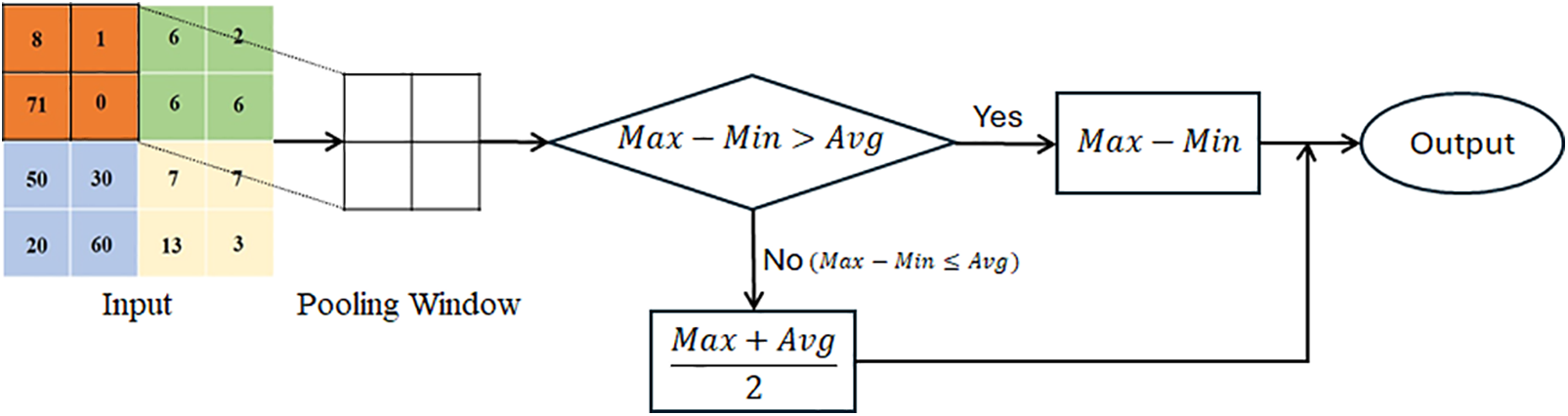
Figure 1: MAM pooling flow scheme

According to Eq. (4), by selecting a value between the average and maximum (Eq. (5)) from the pixel values in the part to be obtained by using a certain filter in a certain image, a new feature map is created containing more prominent features of the feature map.

Avg<MAM≤Max(5)

By producing values greater than the average value in all cases and equal to the maximum value in some cases, an optimal output value between the average and maximum is obtained. According to Eq. (4):

•   Max-Min > Avg (in cases where the difference between the maximum and minimum pixel values in the pooling region is greater than the average): The output value converges to the maximum at pixel values where maximum and minimum values are distant from each other, and to the average at pixel values where they are closer to each other. The larger the difference between the maximum and minimum, the closer to the maximum an output value is obtained, and the smaller it is, the closer to the average an output value is obtained. As the difference between the maximum and minimum increases, it converges more to the maximum, and in some cases, the maximum value is produced. As the difference between the maximum and minimum decreases, it converges to a value between the maximum and average, and in some cases, values closer to the average are produced.

•   Max-Min ≤ Avg (in cases where the difference between the maximum and minimum pixel values in the pooling region is less than or equal to the average): An output value is always produced as the average of the maximum and average values.

In the maximum pooling method, a certain amount of information loss occurs because only the most prominent features from each region are emphasized, and finer details are neglected. In the average pooling method, low activation signals occur because finer details from each region are included in the average, and prominent features are neglected. In the proposed MAM pooling method, a feature map between the maximum and average is created to prevent information loss due to the maximum pooling method neglecting fine details and the formation of low activation signals due to the average pooling method ignoring prominent features. In this way, these disadvantages in the maximum and average pooling methods have become important advantages of the proposed MAM pooling method.

However, the proposed MAM pooling method offers many new contributions to this field. Instead of the maximum and average value, it chooses between the maximum and average, which is not constant but varies according to the data. In this way, it helps the model to generalize better by reducing overfitting, to reduce the dimension more effectively by minimizing information loss, and to increase the performance of the model by better capturing different types of information. Producing an output value locally between the maximum and average expands the information coverage area by ensuring that the information in the feature map is covered in a wider area. It also makes the model more robust against small displacements, reducing performance drops caused by displacements of objects in the images. Therefore, while creating the output value in this pooling method, more prominent (most important, finely detailed, smoother transition) pixel features of the feature map are determined compared to other traditional pooling methods, thus minimizing information loss. However, in this pooling method, determining the location of objects is facilitated without any loss in the contrast feature of the objects in object recognition and the formation of low activation signals is prevented.

Fig. 2 shows an example of Max, Avg, Min, and Proposed MAM pooling applied to an input image. By applying a 2 × 2 pool size and 2 × 2 stride to the feature map with 4 × 4 pixel values coming from the convolution layer, a new feature map with 2 × 2 matrix dimensions was created. When this feature map is examined, it is seen that an output value between the maximum and average is always obtained in the MAM pooling method. For example, in the region where the pixel values “8, 1, 71, 0” are located, the maximum value is 71, the average value is 20, and the minimum value is 0. The maximum and minimum difference is 71 − 0 = 71. Since this value is greater than the average value (71 > 20), the value of 71 (exactly the maximum) was obtained by taking the maximum and minimum difference with MAM pooling. In the region where the pixel values “7, 7, 13, 3” are located, the maximum value is 13, the average value is 7.5, and the minimum value is 3. The maximum and minimum difference is 13 − 3 = 10. Since this value is greater than the average value (10 > 7.5), the value of 10 (closer to the average) was obtained by taking the maximum and minimum difference with MAM pooling. Therefore, in the pooling region, there was convergence to the maximum in pixel values where the maximum and minimum values were distant from each other, and to the average in pixel values where they were closer, as in these two examples. In the region where the pixel values “6, 2, 6, 6” are located, the maximum value is 6, the average value is 5, and the minimum value is 2. The maximum and minimum difference is 6 − 2 = 4. Since this value is less than or equal to the average value (4 ≤ 5), the value of 5.5 was obtained by averaging the maximum and average values with MAM pooling. Likewise, in the region where the pixel values “50, 30, 20, 60” are located, the maximum value is 60, the average value is 40, and the minimum value is 20. The maximum and minimum difference is 60 − 20 = 40. Since this value is less than or equal to the average value (40 ≤ 40), the value of 50 was obtained by averaging the maximum and average values with MAM pooling. Therefore, in the pooling region, an output value was always obtained exactly in the middle of the maximum and average, as in these two examples. Thus, the proposed MAM pooling method produces a more prominent (more important, finely detailed, smoother transition) feature map between the average and maximum.

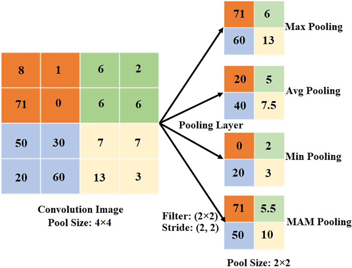
Figure 2: Illustration of Max/Avg/Min/MAM pooling with a pooling area of size 2 × 2

3.2 Dataset

In this study, publicly available CIFAR-10/CIFAR-100 [53] and MNIST [54] datasets were used to determine the success of the proposed MAM pooling and other traditional pooling methods.

CIFAR-10 dataset: It consists of 10 different classes with dimensions of 32 × 32 × 3 pixels. There are 60,000 images in total, 6000 in each class. 50,000 are reserved for training and 10,000 are reserved for testing of the images in the dataset.

CIFAR-100 dataset: It consists of 100 different classes with dimensions of 32 × 32 × 3 pixels. There are 60,000 images in total, 600 in each class. 50,000 are reserved for training and 10,000 are reserved for testing of the images in the dataset.

MNIST dataset: It consists of 10 different classes with dimensions of 28 × 28 × 1 pixels. There are a total of 70,000 images consisting of different numbers of images in each class. 60,000 are reserved for training and 10,000 are reserved for testing of the images in the dataset.

Sample images of these datasets are given in Fig. 3.

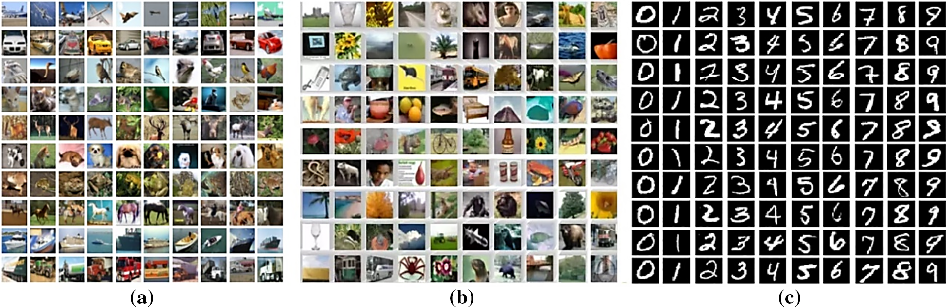
Figure 3: Dataset sample images (a) CIFAR-10 (b) CIFAR-100 (c) MNIST

3.3 Training Parameters

To determine the success of the MAM pooling method proposed in this study, experiments were conducted using the same environment and the same training parameters. Pixel values of the images in the dataset were used at scale values of 0–255. The mini batch size was selected as 128 and the optimization algorithm was selected as Stochastic Gradient Descent (SGD), and the models were trained for 50 epochs. Additionally, the parameter values of all other network layers are set by default.

3.4 Metrics

In this study, the values taken into consideration to determine the classification success of pooling methods are as follows: true positive (tp), false positive (fp), true negative (tn) and false negative (fn). Mathematical expressions given in Eq. (6) through (9) were used to determine model accuracy, precision, recall, and F1-score.

Accuracy=tp+tntp+fp+fn+tn(6)

Precision=tptp+fp(7)

Recall=tptp+fn(8)

F1−score=2∗Precision∗RecallPrecision+Recall(9)

4  Results and Discussion

In this study, the LeNet-5 [54] model was trained and tested on CIFAR-10, CIFAR-100, and MNIST datasets to determine the success of pooling methods. In these training and testing processes, maximum, average, minimum, and recommended MAM pooling methods were applied separately after each convolution layer in the LeNet-5 model. To determine the success accuracy of the pooling method, the experimental results were repeated 5 times for each pooling method and their average was taken.

According to the experimental results obtained, the test success accuracies obtained because of training the LeNet-5 model 5 times on the CIFAR-10 dataset with all pooling methods discussed in the study are shown in Table 1, and the average accuracy success graphs are shown in Fig. 4.

Figure 4: Average accuracy success graph of pooling methods on CIFAR-10 dataset

When Table 1 and Fig. 4 are examined, using the CIFAR-10 dataset in the LeNet-5 model, each pooling method was subjected to training and testing 5 times with pool sizes of 2 × 2, 3 × 3, 4 × 4, and 5 × 5, and comparisons were made according to the average success accuracies of these 5 tests. has been made. When the results obtained are examined, the proposed MAM pooling method is in the success accuracy of the LeNet-5 model on the CIFAR-10 dataset:

•   Compared to the maximum pooling method, the following rates improved:

2 × 2 pool size is also 1.18%,

3 × 3 pool size is also 3.96%,

4 × 4 pool size is also 3.51%,

5 × 5 pool size is also 2.36%.

Compared to the average pooling method, the following rates improved:

-   2 × 2 pool size is also 6.93%,

-   3 × 3 pool size is also 11.41%,

-   4 × 4 pool size is also 12.33%,

-   5 × 5 pool size is also 15.9%.

Compared to the minimum pooling method, the following rates improved:

-   2 × 2 pool size is also 1.63%,

-   3 × 3 pool size is also 3.7%,

-   4 × 4 pool size is also 3.26%,

-   5 × 5 pool size is also 3.15%.

According to these results, the proposed MAM pooling method showed better performance than other traditional pooling methods considered in the study on the CIFAR-10 dataset. In the training conducted on the CIFAR-10 dataset in the LeNet-5 model, the proposed MAM pooling method was successful not only in one pool size but also in other pool sizes.

The test success accuracies obtained because of training the LeNet-5 model 5 times on the CIFAR-100 dataset with all pooling methods discussed in the study are shown in Table 2, and the average accuracy success graphs are shown in Fig. 5.

Figure 5: Average accuracy success graph of pooling methods on CIFAR-100 dataset

When Table 2 and Fig. 5 are examined, using the CIFAR-100 dataset in the LeNet-5 model, each pooling method was subjected to training and testing 5 times with pool sizes of 2 × 2, 3 × 3, 4 × 4, and 5 × 5, and comparisons were made according to the average success accuracies of these 5 tests. has been made. When the results obtained are examined, the proposed MAM pooling method is in the success accuracy of the LeNet-5 model on the CIFAR-100 dataset:

•   Compared to the maximum pooling method, the following rates improved:

2 × 2 pool size is also 2.27%,

3 × 3 pool size is also 2.83%,

4 × 4 pool size is also 3.13%,

5 × 5 pool size is also 3.03%.

Compared to the average pooling method, the following rates improved:

-   2 × 2 pool size is also 6.19%,

-   3 × 3 pool size is also 8.06%,

-   4 × 4 pool size is also 8.24%,

-   5 × 5 pool size is also 9.49%.

Compared to the minimum pooling method, the following rates improved:

-   2 × 2 pool size is also 2.02%,

-   3 × 3 pool size is also 3.13%,

-   4 × 4 pool size is also 2.91%,

-   5 × 5 pool size is also 3.27%.

According to these results, the proposed MAM pooling method showed better performance than other traditional pooling methods considered in the study on the CIFAR-100 dataset. In the training conducted on the CIFAR-100 dataset in the LeNet-5 model, the proposed MAM pooling method was successful not only in one pool size but also in other pool sizes. However, the proposed MAM pooling method performed better than other traditional methods on the CIFAR-100 dataset compared to the CIFAR-10 dataset.

The test success accuracies obtained because of training the LeNet-5 model 5 times on the MNIST dataset with all pooling methods discussed in the study are shown in Table 3, and the average accuracy success graphs are shown in Fig. 6.

Figure 6: Average accuracy success graph of pooling methods on MNIST dataset

When Table 3 and Fig. 6 are examined, using the MNIST dataset in the LeNet-5 model, each pooling method was subjected to training and testing 5 times with pool sizes of 2 × 2, 3 × 3, 4 × 4, and 5 × 5, and comparisons were made according to the average success accuracies of these 5 tests. has been made. When the results obtained are examined, the proposed MAM pooling method is in the success accuracy of the LeNet-5 model on the MNIST dataset:

•   Compared to the maximum pooling method, the following rates improved:

2 × 2 pool size is also 0.12%,

3 × 3 pool size is also 0.16%,

4 × 4 pool size is also 0.45%,

5 × 5 pool size is also 0.44%.

Compared to the average pooling method, the following rates improved:

-   2 × 2 pool size is also 0.54%,

-   3 × 3 pool size is also 1.05%,

-   4 × 4 pool size is also 2.59%,

-   5 × 5 pool size is also 3.96%.

Compared to the minimum pooling method, the following rates improved:

-   2 × 2 pool size is also 0.05%,

-   3 × 3 pool size is also 0.32%,

-   4 × 4 pool size is also 0.56%,

-   5 × 5 pool size is also 0.46%.

According to these results, the proposed MAM pooling method showed better performance than other traditional pooling methods considered in the study on the MNIST dataset. In the training conducted on the MNIST dataset in the LeNet-5 model, the proposed MAM pooling method was successful not only in one pool size but also in other pool sizes.

In all pooling methods discussed in this study, a decrease in performance was observed as the pool size increased. Although it was determined that there was a decrease in success accuracy in the proposed method, like other traditional methods, due to the increase in pool size, it was determined that the proposed method was more successful. When all experimental results were examined, the proposed MAM pooling method showed better performance by producing more appropriate feature maps than other traditional pooling methods on different datasets and at different pool size values.

In addition, some recent studies using the models and datasets used in our study were examined and the results are presented comparatively in Table 4.

When Table 4 is examined, it is seen that the most successful accuracy is obtained with the proposed method when the pool size is 2, regardless of the dataset. As the pool size value increases, the success rate of the proposed method decreases, and its accuracy is lower than other methods. The use of different activation functions other than the methods used in the studies may be a reason affecting this situation. In addition, apart from the successful results obtained with 2 pool sizes, the proposed method was also more successful than other methods with 3 pool sizes on the CIFAR-10 dataset. In 3 pool sizes, Doğan [45] achieved the most successful accuracy in the CIFAR-100 dataset, while Zhao et al. [55] achieved the most successful accuracy in the MNIST dataset. It was observed that the proposed method achieved an accuracy close to the most successful result on the MNIST dataset in 3 pool sizes. In 4 pool sizes, Zhao and Zhang achieved the most successful results, while in 5 pool sizes, Doğan achieved the most successful results. Although the accuracy rates are slightly lower in large pool sizes, results close to other methods were obtained with the proposed method. This reveals that the proposed method is superior to other methods in certain pool sizes and can compete with them in certain pool sizes.

5  Expansion Experiment

Experiments were also carried out on a different model to investigate the effectiveness and validity of the MAM pooling method. To carry out these experiments, studies were carried out on the VGG16 [56] model. There is a minimum input size for the VGG16 model to work and this input size should not be less than 32. Since the MNIST dataset is 28 × 28 in size, the MNIST dataset could not be used in the VGG16 model. In addition, when the pool size is larger than 2, the model does not work because the shape problem occurs in the last layers of the VGG16 model. For this reason, the pool size is set to only 2. CIFAR-10 and CIFAR-100 datasets were used in the expansion experiments, and the proposed MAM pooling method and traditional pooling methods were applied to the pooling layer of the VGG16 model. Experiments performed using the same training parameters specified in the previous sections of the study were repeated 5 times for each pooling method. As a result of the experiments, it was observed that the VGG16 model did not learn from the CIFAR-100 dataset. Therefore, only the experimental results performed with the CIFAR-10 dataset are included. The numerical results obtained as a result of the experiments are given in Table 5, and the average success graphs are given in Fig. 7.

Figure 7: Average success graph of pooling methods in the VGG16 model

When Table 5 and Fig. 7 are examined, it is seen that the proposed MAM pooling method is more successful than other traditional methods in the VGG16 model. While an average accuracy of 72.6% was achieved with the proposed method, an average accuracy of 67.2% was achieved with its closest follower, maximum pooling. It was observed that the proposed method was slower than other methods in terms of computation time. While the fastest computation time was obtained with the average pooling method (24.36 s), the slowest computation time was achieved with the proposed method (27.57 s). However, a very low success rate was achieved with the average pooling method compared to the proposed method. Therefore, the performance increase of the proposed method outweighs the potential increase in computation time. The proposed method performed better than other traditional methods in all metrics except computation time.

6  Conclusion

In this study, a new approach called MAM pooling was developed as an alternative to traditional pooling (maximum, average, and minimum) methods used in convolutional neural networks. To test the success of the developed approach, many experiments were conducted on the LeNet-5 model using three different datasets (CIFAR-10, CIFAR-100, and MNIST). According to experimental results, the proposed MAM pooling method showed superior performance than other traditional methods considered in the study in 2 × 2, 3 × 3, 4 × 4, and 5 × 5 pool sizes.

It has been revealed that the developed MAM pooling method is more interactive than the traditional maximum pooling, average pooling, and minimum pooling methods used in convolutional neural networks and reduces data loss by calculating more appropriate pixel values. In addition, the proposed MAM pooling method highlights the most important, finely detailed, and smoother transition features in the feature maps compared to traditional pooling methods, enabling the location of objects to be determined better, preventing low activation signals, and minimizing information loss. The developed MAM pooling method is planned to be applied to many different model structures and datasets and compared with different pooling methods in the future.

Acknowledgement: None.

Funding Statement: The author received no specific funding for this study.

Availability of Data and Materials: All data generated or analysed during this study are included in this published article.

Conflicts of Interest: The author declares that he has no conflicts of interest to report regarding the present study.

References

1. Mariani MM, Machado I, Magrelli V, Dwivedi YK. Artificial intelligence in innovation research: a systematic review, conceptual framework, and future research directions. Technovation. 2023;122:102623. doi:10.1016/j.technovation.2022.102623. [Google Scholar] [CrossRef]

2. Zahlan A, Ranjan RP, Hayes D. Artificial intelligence innovation in healthcare: literature review, exploratory analysis, and future research. Technol Soc. 2023;74:102321. doi:10.1016/j.techsoc.2023.102321. [Google Scholar] [CrossRef]

3. Mariani MM, Machado I, Nambisan S. Types of innovation and artificial intelligence: a systematic quantitative literature review and research agenda. J Bus Res. 2023;155:113364. doi:10.1016/j.jbusres.2022.113364. [Google Scholar] [CrossRef]

4. Katzman BD, van der Pol CB, Soyer P, Patlas MN. Artificial intelligence in emergency radiology: a review of applications and possibilities. Diagn Interv Imag. 2023;104(1):6–10. doi:10.1016/j.diii.2022.07.005. [Google Scholar] [PubMed] [CrossRef]

5. Dorr DA, Adams L, Embí P. Harnessing the promise of artificial intelligence responsibly. JAMA. 2023;329(16):1347–8. doi:10.1001/jama.2023.2771. [Google Scholar] [PubMed] [CrossRef]

6. Taye MM. Understanding of machine learning with deep learning: architectures, workflow, applications and future directions. Computers. 2023;12(5):91. doi:10.3390/computers12050091. [Google Scholar] [CrossRef]

7. Kaveh M, Mesgari MS. Application of meta-heuristic algorithms for training neural networks and deep learning architectures: a comprehensive review. Neural Process Lett. 2023;55(4):4519–622. doi:10.1007/s11063-022-11055-6. [Google Scholar] [PubMed] [CrossRef]

8. Kaya V. Classification of waste materials with a smart garbage system for sustainable development: a novel model. Front Environ Sci. 2023;11:1–6. [Google Scholar]

9. Giudici P, Centurelli M, Turchetta S. Artificial intelligence risk measurement. Expert Syst Appl. 2024;235:121220. doi:10.1016/j.eswa.2023.121220. [Google Scholar] [CrossRef]

10. Sarker IH. Machine learning for intelligent data analysis and automation in cybersecurity: current and future prospects. Ann Data Sci. 2023;10(6):1473–98. doi:10.1007/s40745-022-00444-2. [Google Scholar] [CrossRef]

11. Zhang Y, Zhao M. Cloud-based in-situ battery life prediction and classification using machine learning. Energy Storage Mater. 2023;57:346–59. doi:10.1016/j.ensm.2023.02.035. [Google Scholar] [CrossRef]

12. Alrayes FS, Asiri MM, Maashi MS, Nour MK, Rizwanullah M, Osman AE, et al. Waste classification using vision transformer based on multilayer hybrid convolution neural network. Urban Clim. 2023;49:101483. doi:10.1016/j.uclim.2023.101483. [Google Scholar] [CrossRef]

13. Ejegwa PA, Ahemen S. Enhanced intuitionistic fuzzy similarity operators with applications in emergency management and pattern recognition. Granul Comput. 2023;8(2):361–72. doi:10.1007/s41066-022-00334-1. [Google Scholar] [CrossRef]

14. Mirbod M, Shoar M. Intelligent concrete surface cracks detection using computer vision, pattern recognition, and artificial neural networks. Procedia Comput Sci. 2023;217:52–61. doi:10.1016/j.procs.2022.12.201. [Google Scholar] [CrossRef]

15. Dang M, Wang H, Li Y, Nguyen TH, Tightiz L, Xuan-Mung N, et al. Computer vision for plant disease recognition: a comprehensive review. The Bot Rev. 2024;90:1–61. [Google Scholar]

16. Ahmed SF, Alam MSB, Hassan M, Rozbu MR, Ishtiak T, Rafa N, et al. Deep learning modelling techniques: current progress, applications, advantages, and challenges. Artif Intell Rev. 2023;56(1113521–617. doi:10.1007/s10462-023-10466-8. [Google Scholar] [CrossRef]

17. Li N, Ma L, Yu G, Xue B, Zhang M, Jin Y. Survey on evolutionary deep learning: principles, algorithms, applications, and open issues. ACM Comput Surv. 2023;56(2):1–34. [Google Scholar]

18. Narayan V, Awasthi S, Fatima N, Faiz M, Srivastava S. Deep learning approaches for human gait recognition: a review. In: 2023 International Conference on Artificial Intelligence and Smart Communication (AISC); 2023 Jan 27–29; Greater Noida, India: IEEE. p. 763–8. [Google Scholar]

19. Malhotra R, Singh P. Recent advances in deep learning models: a systematic literature review. Multimed Tools Appl. 2023;82(29):44977–5060. doi:10.1007/s11042-023-15295-z. [Google Scholar] [CrossRef]

20. Sathio AA, Rind MM, Lakhan A. Deep learning algorithms: clustering and classifications for multimedia data. In: Deep learning for multimedia processing applications. 1st edition, Boca Raton: CRC Press; 2024. p. 114–45. [Google Scholar]

21. Taye MM. Theoretical understanding of convolutional neural network: concepts, architectures, applications, future directions. Computation. 2023;11(3):52. doi:10.3390/computation11030052. [Google Scholar] [CrossRef]

22. Kshatri SS, Singh D. Convolutional neural network in medical image analysis: a review. Arch Comput Methods Eng. 2023;30(4):2793–810. doi:10.1007/s11831-023-09898-w. [Google Scholar] [CrossRef]

23. Bhatti UA, Tang H, Wu G, Marjan S, Hussain A. Deep learning with graph convolutional networks: an overview and latest applications in computational intelligence. Int J Intell Syst. 2023;2023(1):8342104. [Google Scholar]

24. Bharadiya J. Convolutional neural networks for image classification. Int J Innov Sci Res Technol. 2023;8(5):673–7. [Google Scholar]

25. O’shea K, Nash R. An introduction to convolutional neural networks. arXiv preprint arXiv:1511.08458. 2015. [Google Scholar]

26. Habibi Aghdam H, Jahani Heravi E. Convolutional neural networks. In: Guide to convolutional neural networks. Cham: Springer; 2017. p. 85–130. [Google Scholar]

27. Albawi S, Mohammed TA, Al-Zawi S. Understanding of a convolutional neural network. In: 2017 International Conference on Engineering and Technology (ICET); 2017 Aug 21–23; Antalya, Turkey: IEEE. p. 1–6. [Google Scholar]

28. Gu J, Wang Z, Kuen J, Ma L, Shahroudy A, Shuai B, et al. Recent advances in convolutional neural networks. Pattern Recognit. 2018;77:354–77. doi:10.1016/j.patcog.2017.10.013. [Google Scholar] [CrossRef]

29. Vakalopoulou M, Christodoulidis S, Burgos N, Colliot O, Lepetit V. Deep learning: basics and convolutional neural networks (CNNs). In: Colliot O, editor. Machine learning for brain disorders. New York: Humana; 2023. p. 77–115. [Google Scholar]

30. Aloysius N, Geetha M. A review on deep convolutional neural networks. In: International Conference on Communication and Signal Processing (ICCSP); 2017 Apr 06–08; Chennai, India: IEEE. p. 588–92. [Google Scholar]

31. Gholamalinezhad H, Khosravi H. Pooling methods in deep neural networks, a review. arXiv preprint arXiv:2009.07485. 2009. [Google Scholar]

32. Zafar A, Aamir M, Mohd Nawi N, Arshad A, Riaz S, Alruban A, et al. A comparison of pooling methods for convolutional neural networks. Appl Sci. 2022;12(17):8643. doi:10.3390/app12178643. [Google Scholar] [CrossRef]

33. LeCun Y, Bengio Y, Hinton G. Deep learning. Nature. 2015;521(7553):436–44. doi:10.1038/nature14539. [Google Scholar] [PubMed] [CrossRef]

34. Guo Y, Liu Y, Oerlemans A, Lao S, Wu S, Lew MS. Deep learning for visual understanding: a review. Neurocomputing. 2016;187:27–48. doi:10.1016/j.neucom.2015.09.116. [Google Scholar] [CrossRef]

35. Kim P. Convolutional neural network. In: Kim P, editor. MATLAB deep learning: with machinelearning, neural networks and artificial intelligence. New York: Apress; 2017. p. 121–47. [Google Scholar]

36. Shi Z, Ye Y, Wu Y. Rank-based pooling for deep convolutional neural networks. Neural Netw. 2016;83: 21–31. doi:10.1016/j.neunet.2016.07.003. [Google Scholar] [PubMed] [CrossRef]

37. Galanis NI, Vafiadis P, Mirzaev KG, Papakostas GA. Convolutional neural networks: a roundup and benchmark of their pooling layer variants. Algorithms. 2022;15(11):391. doi:10.3390/a15110391. [Google Scholar] [CrossRef]

38. Satti P, Sharma N, Garg B. Min-max average pooling based filter for impulse noise removal. IEEE Signal Process Lett. 2020;27:1475–9. doi:10.1109/LSP.2020.3016868. [Google Scholar] [CrossRef]

39. Song Z, Liu Y, Song R, Chen Z, Yang J, Zhang C, et al. A sparsity-based stochastic pooling mechanism for deep convolutional neural networks. Neural Netw. 2018;105:340–5. doi:10.1016/j.neunet.2018.05.015. [Google Scholar] [PubMed] [CrossRef]

40. Devi N, Borah B. Cascaded pooling for convolutional neural networks. In: 2018 Fourteenth International Conference on Information Processing (ICINPRO); 2018 Dec 21–23; Bangalore, India: IEEE. p. 1–5. [Google Scholar]

41. Nirthika R, Manivannan S, Ramanan A, Wang R. Pooling in convolutional neural networks for medical image analysis: a survey and an empirical study. Neural Comput Appl. 2022;34(7):5321–47. doi:10.1007/s00521-022-06953-8. [Google Scholar] [PubMed] [CrossRef]

42. Özdemir C. Avg-topk: a new pooling method for convolutional neural networks. Expert Syst Appl. 2023;223:119892. doi:10.1016/j.eswa.2023.119892. [Google Scholar] [CrossRef]

43. Park J, Kim JY, Huh JH, Lee HS, Jung SH, Sim CB. A novel on conditional min pooling and restructured convolutional neural network. Electronics. 2021;10(19):2407. doi:10.3390/electronics10192407. [Google Scholar] [CrossRef]

44. Yildirim M. Analog circuit architecture for max and min pooling methods on image. Analog Integr Circuits Signal Process. 2021;108(1):119–24. doi:10.1007/s10470-021-01842-x. [Google Scholar] [CrossRef]

45. Doğan Y. Which pooling method is better: max, avg, or concat (Max, Avg). Commun Fac Sci Univ Ank A2–A3 Phys Sci Eng. 2023;66(1):95–117. doi:10.33769/aupse.1356138. [Google Scholar] [CrossRef]

46. Hyun J, Seong H, Kim E. Universal pooling–a new pooling method for convolutional neural networks. Expert Syst Appl. 2021;180:115084. doi:10.1016/j.eswa.2021.115084. [Google Scholar] [CrossRef]

47. Sun M, Song Z, Jiang X, Pan J, Pang Y. Learning pooling for convolutional neural network. Neurocomputing. 2017;224:96–104. doi:10.1016/j.neucom.2016.10.049. [Google Scholar] [CrossRef]

48. Jie HJ, Wanda P. RunPool: a dynamic pooling layer for convolution neural network. Int J Comput Intell Syst. 2020;13(1):66–76. doi:10.2991/ijcis.d.200120.002. [Google Scholar] [CrossRef]

49. Lukman A, Saputro WT, Seniwati E. Improving performance convolutional neural networks using modified pooling function. MATRIK: J Manaj Tech Inform Rekayasa Comput. 2024;23(2):343–52. doi:10.30812/matrik.v23i2. [Google Scholar] [CrossRef]

50. Skourt BA, El Hassani A, Majda A. Mixed-pooling-dropout for convolutional neural network regularization. J King Saud Univ-Comput Inf Sci. 2022;34(8):4756–62. [Google Scholar]

51. Boxue Z, Qi Z, Wenquan F, Shuchang L. AlphaMEX: a smarter global pooling method for convolutional neural networks. Neurocomputing. 2018;321:36–48. doi:10.1016/j.neucom.2018.07.079. [Google Scholar] [CrossRef]

52. Singh P, Raj P, Namboodiri VP. EDS pooling layer. Image Vis Comput. 2020;98:103923. doi:10.1016/j.imavis.2020.103923. [Google Scholar] [CrossRef]

53. Krizhevsky A. Learning multiple layers of features from tiny images (Master’s Thesis). Toronto University: Canada; 2009. [Google Scholar]

54. LeCun Y, Bottou L, Bengio Y, Haffner P. Gradient-based learning applied to document recognition. Proc IEEE. 1998;86(11):2278–324. doi:10.1109/5.726791. [Google Scholar] [CrossRef]

55. Zhao L, Zhang Z. A improved pooling method for convolutional neural networks. Sci Rep. 2024;14(1):1589. doi:10.1038/s41598-024-51258-6. [Google Scholar] [PubMed] [CrossRef]

56. Simonyan K, Zisserman A. Very deep convolutional networks for large-scale image recognition. arXiv preprint arXiv:1409.1556. 2014. [Google Scholar]