
 Submit a Paper
 Propose a Special lssue
 Open Access
ARTICLE

Numerical Analysis of Bacterial Meningitis Stochastic Delayed Epidemic Model through Computational Methods
1 Department of Mathematics, National College of Business Administration and Economics, Lahore, 54660, Pakistan
2 Department of Mathematics, Applied College, Mahayl Assir, King Khalid University, Abha, 62529, Saudi Arabia
3 Department of Physical Sciences, The University of Chenab, Gujrat, 50700, Pakistan
4 Department of Mathematics & Statistics, College of Science, King Faisal University, P.O. Box 400, Al-Ahsa, 31982, Saudi Arabia
5 Department of Computer Science and Mathematics, Lebanese American University, Beirut, 1102-2801, Lebanon
6 Department of Mathematics, Faculty of Science and Technology, University of Central Punjab, Lahore, 54000, Pakistan
7 Department of Mathematics and Statistics, University of Lahore, Lahore, 54000, Pakistan
* Corresponding Authors: Umar Shafique. Email: ; Emad Fadhal. Email:
(This article belongs to the Special Issue: Mathematical Aspects of Computational Biology and Bioinformatics-II)
Computer Modeling in Engineering & Sciences 2024, 141(1), 311-329. https://doi.org/10.32604/cmes.2024.052383
Received 31 March 2024; Accepted 28 June 2024; Issue published 20 August 2024
 View Full Text
 Download PDF
Abstract
Based on the World Health Organization (WHO), Meningitis is a severe infection of the meninges, the membranes covering the brain and spinal cord. It is a devastating disease and remains a significant public health challenge. This study investigates a bacterial meningitis model through deterministic and stochastic versions. Four-compartment population dynamics explain the concept, particularly the susceptible population, carrier, infected, and recovered. The model predicts the nonnegative equilibrium points and reproduction number, i.e., the Meningitis-Free Equilibrium (MFE), and Meningitis-Existing Equilibrium (MEE). For the stochastic version of the existing deterministic model, the two methodologies studied are transition probabilities and non-parametric perturbations. Also, positivity, boundedness, extinction, and disease persistence are studied rigorously with the help of well-known theorems. Standard and nonstandard techniques such as Euler Maruyama, stochastic Euler, stochastic Runge Kutta, and stochastic nonstandard finite difference in the sense of delay have been presented for computational analysis of the stochastic model. Unfortunately, standard methods fail to restore the biological properties of the model, so the stochastic nonstandard finite difference approximation is offered as an efficient, low-cost, and independent of time step size. In addition, the convergence, local, and global stability around the equilibria of the nonstandard computational method is studied by assuming the perturbation effect is zero. The simulations and comparison of the methods are presented to support the theoretical results and for the best visualization of results.Keywords
Meningitis caused by bacteria results in inflammation of the membranes surrounding the brain and spinal cord. The most common bacteria that cause meningitis are Streptococcus pneumoniae, Neisseria meningitidis, and Haemophilus influenzae type b. The signs and symptoms of bacterial meningitis include a sharply rising temperature, headache, stiff neck, and light sensitivity. Serious complications such as brain damage or death are caused by bacterial meningitis, so swift medical attention is crucial. Specific bacterial strains that cause meningitis can be controlled by effective vaccination [1]. Medical officers usually prescribe medicines such as ceftriaxone or cefotaxime to target invading bacteria and cure bacterial meningitis. Corticosteroids such as dexamethasone may be dispensed to decrease inflammation. Shin et al. [2] studied a mathematical model incorporating hospitalization and treatment factors. Madaki et al. [3] designed a mathematical model of meningococcal meningitis in Nigeria. In [4,5], the study was based on acute bacterial meningitis in adults. In [6,7], the study was designed on reviewed reports from the WHO and a model that describes a bacterial disease. Mohanty et al. [8] explained the different types of vaccines and preventive measures to control bacterial meningitis in Sweden. Van et al. [9] investigated in great detail all the stages of bacterial meningitis, from its initiation to its outbreak, and formulated various preventive measures to control it. Rauti et al. [10] developed a mathematical model for preventing bacterial meningitis in animals that can be employed to prevent infections of this deadly disease. Hou et al. [11] presented a dynamic model for preventing bacterial meningitis in young children using metagenomic sequencing, in which this approach can largely control the disease. Signing et al. [12] created a mathematical model that can visualize the changes caused by bacterial meningitis disease and their effect and can be treated accordingly to control the disease. Afridi et al. [13] identified different preventive measures and vaccines while reviewing bacterial meningitis cases brought to a civil hospital in Pakistan. Buonomo et al. [14] reported that the meningitis outbreak in Nigeria is analyzed using a behavior-focused vaccination model. This strategy considers behavioral elements while evaluating immunization strategies. It contributes to developing more effective preventative methods tailored to Nigeria’s socioeconomic environment and sheds light on the dynamics of meningitis transmission. Babatunde et al. [15] employed an online tool using logistic regression to predict cerebrospinal meningitis incidence is currently being developed. The goal of this initiative is to enhance illness management and early diagnosis. The initiative uses statistical modeling to evaluate relevant data, which can give useful information to policymakers and healthcare practitioners. Bradley et al. [16] reviewed the English medical literature and introduced a method that can be utilized to control bacterial meningitis. Choi et al. [17] created a mathematical model using AI to control bacterial meningitis in the future. Chen et al. [18] stated that it is essential to identify clinical and laboratory parameters to control bacterial meningitis disease. Olu et al. [19] created a mathematical model that can be very useful to control the growing epidemic of bacterial meningitis in the population. In [20], the authors studied a new analyzing technique for nonlinear time fractional Cauchy reaction-diffusion model equations. The stochastic epidemic models with delays are constructed given the need to incorporate the proper transmission process of the epidemic in any populace. These models make use of such lags and lags to mimic the period within which a person gets exposed and becomes infectious and lags in the uptake and efficacy of the implemented interventions. These models help to explain why so many epidemics exhibit cyclic behavior, this is in terms of the waves and seasonality that characterize many epidemics, and delay, noise, and heterogeneity are shown to play crucial roles. Also, the stochastic with delay effect results close to the actual statistics of the problem. So, in the present study, we extend the deterministic model in the sense of stochastic with delay. Then our new system was based on stochastic delay differential equations (SDDEs), due to complexity, we used standard and nonstandard methods to understand the dynamics of bacterial meningitis.
The structure of the paper is as follows: a brief overview and thorough analysis of bacterial meningitis-like disorders found in the literature are provided in Section 1. Establishing the delayed model and the ensuing mathematical analysis are the focus of Section 2. Section 3 presents the stochastic formulation of the model and the extinction and persistence of the model. The nonstandard computational method with delay and stochastic is introduced in Section 4, along with its global and local stability assessment. Numerical simulations and the presentation of the results are the explicit focus of Section 5. The final opinions provide a comprehensive conclusion of the work in Section 6.
The dynamics of population theory is a foundation for the model’s development. The classes susceptible S(t), carrier C(t), infected I(t), and recovered R(t) add up to the population N(t), and they use the law of mass action to represent the condition of bacterial meningitis (Fig. 1).
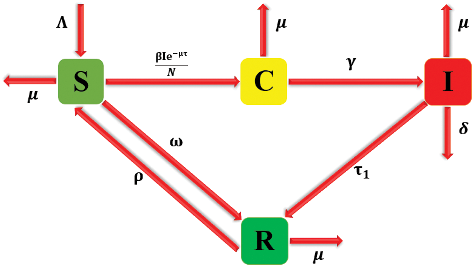
Figure 1: Flow of bacterial meningitis [3]
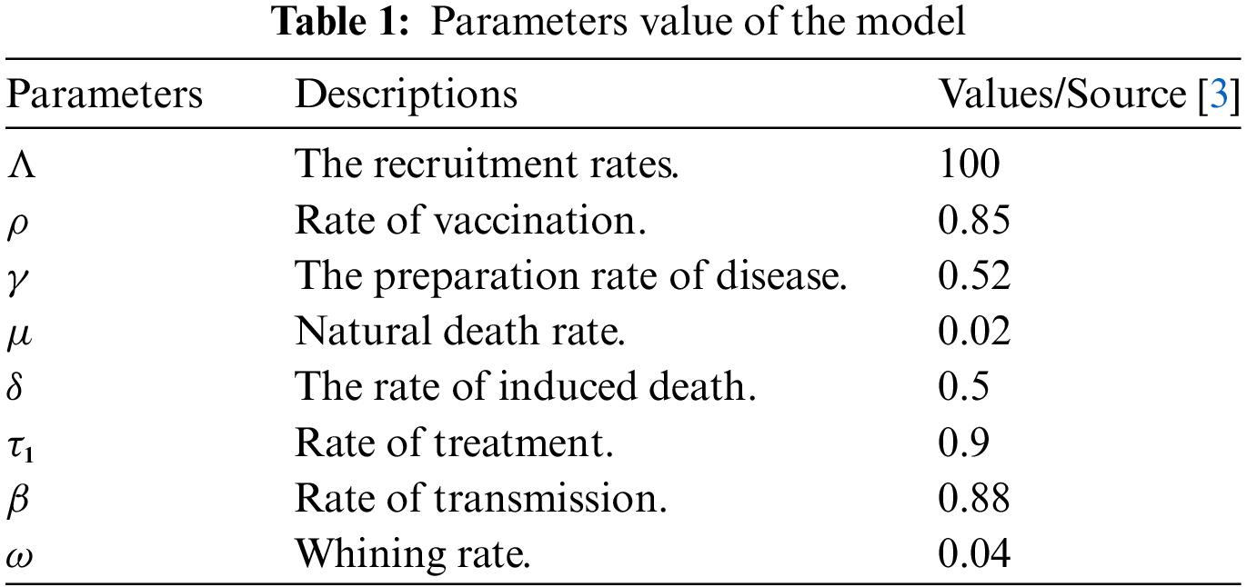
The parameter values of the constants are shown as follows in Table 1.
The law of mass action specifies the continuous model based on the presumptions. The transmission flow of bacterial meningitis-type disease is determined using the nonlinear delayed differential equations (DDEs) as follows:
with the initial assumptions
For the critical analysis of the model to continue, all of the variables
This section presents a concise analysis of the equilibria in the delayed model for bacterial meningitis, i.e., Meningitis-Free Equilibrium (
The systems (1)–(4) incorporate the advanced matrix approach to compute the threshold number
The spectral radius of
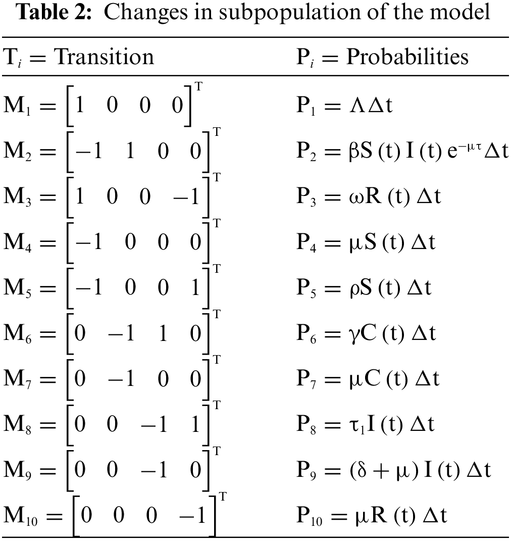
3 Transition Probabilities of the Delayed Model
Let us examine the vector
Here,
drift
Eq. (6) is the stochastic differential equation, where
This section discusses a conventional numerical technique for approximating a stochastic delayed model’s result of (6). In this regard,
for each n ∈
The mean of each ∆
The system of stochastic delayed differential equations (SDDEs) is a mathematical model that describes the evolution of a set of variables over time, where the equations involve both deterministic time delays and stochastic (random) components. Where the stochastic term
Subject to non-negative initial conditions
3.2.1 Positivity and Boundedness
Let us examine a probability space represented as
The norm
This study analyzes the collection of all non-negative functions V (U, t) defined on
As,
If Q acts on a function
where
Theorem 1. For a given model (7)–(10) and initial values
Proof: Based on Ito’s formula, the model (7)–(10) has a unique local positive solution in the interval
Next, this study demonstrates that the provided model (7)–(10) possesses a solution in the global sense, specifically when
Assume that
where this study sets
Thereafter, the limit
If this condition is not met, then there are positive values T and ε, where T is more than zero, and ε is between 0 and 1, such that
there is an integer
Define a
The following can be calculated using Ito’s formula:
For simplification, this study assumes
Assume
where
Set
Hence,
Thereafter, the following can be obtained:
The indicator function is represented by
as desired.
3.2.2 Extinction and Persistence
Definition: Consider
If
Let us introduce
Theorem 2. If
Proof: Given the initial data
Let,
Notice that,
4 Nonstandard Computational Method
The proposed non-parametric perturbation model’s first Eq. (10) can be stated using an unconventional computing technique; specifically, Eqs. (10)–(13) could be solved using a stochastic nonstandard finite difference technique.
For the stochastic NSFD approach, the structure of the equation is as follows:
The system (10)–(13) can be broken down using the stochastic NSFD process, and the complete system can then be written as follows:
where
Theorem 3. There is only one positive solution
Proof: The proof is easily verifiable due to the non-negative nature of the restriction of biological problems.
Theorem 4. For the region
Proof: The system (25) to (28) can be deconstructed as follows:
After adding the above system of equations, the following can be obtained:
4.2 Local Stability Analysis of Nonstandard Computational Method
Consider the right-hand side of the Eqs. (25)–(28) functions F, G, H, and P and
It is commonly understood that a system of the forms (25)–(28) converges to the model’s optimal state if and only if the Jacobian’s spectral radius, J,
Theorem 5. The meningitis-free equilibrium (
Proof: The Jacobian matrix (29) at
Using the definition of
Theorem 6. The meningitis existing equilibrium (
Proof: The Jacobian matrix (29) at
Lemma 1. For the quadratic equation
(i)
(ii)
(iii)
Proof: The proof is straightforward.
4.3 Global Stability Analysis of Nonstandard Computational Method
Theorem 7. The meningitis-free equilibrium (
Proof: Let us consider the Lyapunov function as follows:
where
Using Entasu et al. [21] criterion
Definitely,
Theorem 8. The meningitis existing equilibrium (
Proof: In order to analyze the sufficient condition for global stability, the Lyapunov functions are defined as follows:
where
Hence,
This section compares known numerical approaches to a stochastic nonstandard computational method with existing methods such as Euler Maruyama, stochastic Euler, and stochastic Runge Kutta in the literature for the particular real-world problem.
Fig. 2a,b compares the infected class of the nonstandard computational method in the sense of delay with stochastic and the Euler Maruyama method. At ℎ = 0.01, both methods demonstrate convergence in Fig. 2a. When the step size increases to ℎ = 0.5, the Euler Maruyama method exhibits divergence, whereas the nonstandard computational method in the sense of delay with stochastic maintains convergence, as illustrated in Fig. 2b. Similarly, Fig. 2c,d compares the infected class of the nonstandard computational method in the sense of delay with stochastic and stochastic Euler methods. At ℎ = 0.01, both methods converge in Fig. 2c; however, with an increment in step size to ℎ = 0.7, the stochastic Euler method diverges, while the nonstandard computational method in the sense of delay with stochastic method-maintained convergence, as depicted in Fig. 2d. Figs. 2e,f compares the infected class of the nonstandard computational method in the sense of delay with stochastic and stochastic Runge Kutta methods. At ℎ = 0.1, convergence is a numerical analysis of the stochastic delayed bacterial meningitis epidemic model observed in both methods in Fig. 2e; however, with an increase in step size to ℎ = 1.0, the stochastic Runge Kutta method diverges. In contrast, the nonstandard computational method in the sense of delay with the stochastic method continues to converge, as indicated in Fig. 2f. Fig. 3a depicts the impact of delay on the susceptible class of the model at various values 𝜏 = 0.1, 0.2, 0.3, 0.4, 0.5. Fig. 3b shows the effect of delay on the infected class of the model at different values 𝜏 = 0.1, 0.2, 0.3, 0.4, 0.5, illustrating a gradual decrease in the disease from the infected class over time. Fig. 4 shows a comparison of the double delay effect with the reproduction number. The increase in delay value may decrease the value of the reproduction number and vice versa. The decrease in reproduction number shows that the disease has been controlled in the population.
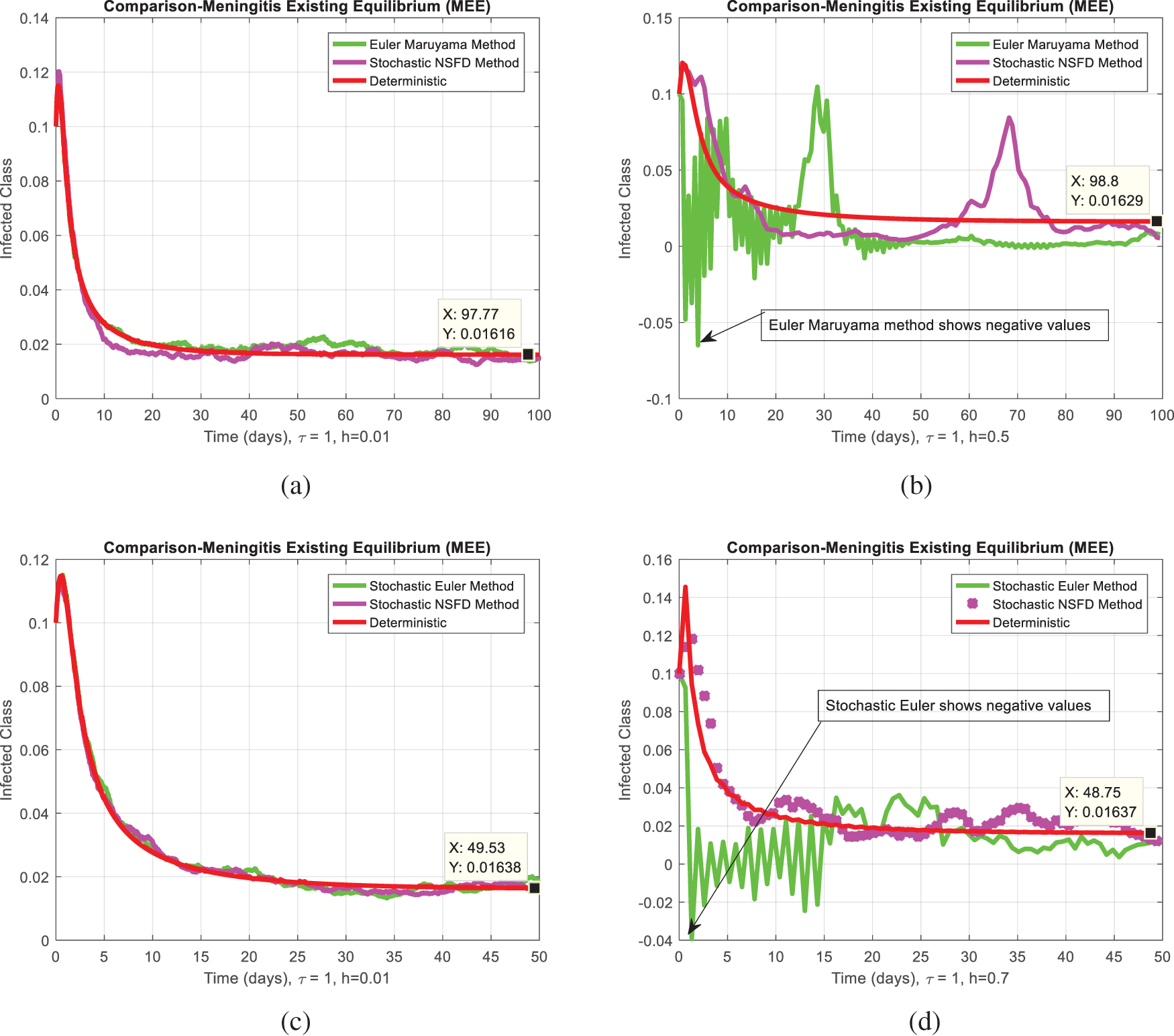
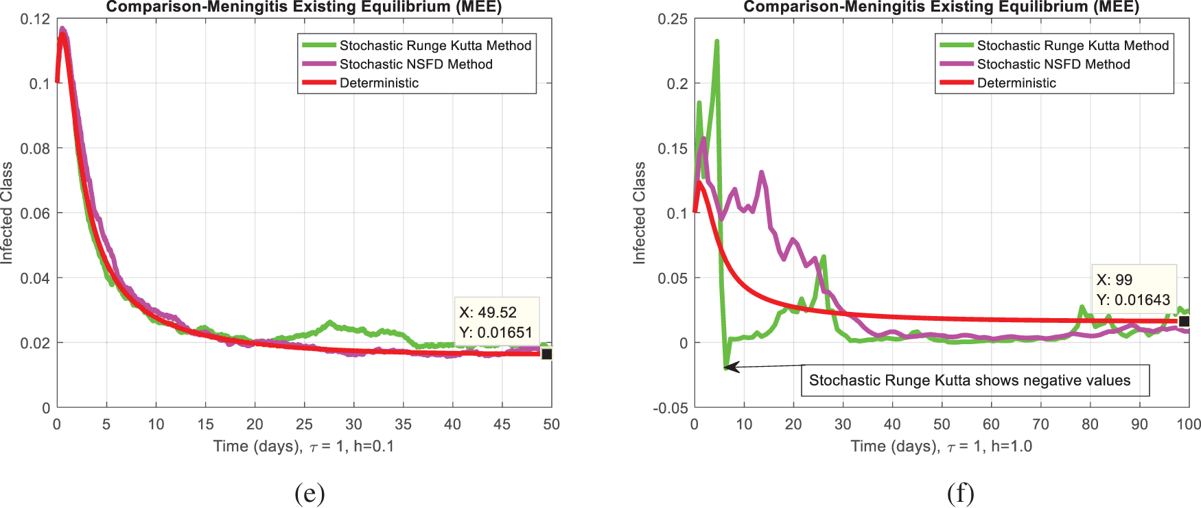
Figure 2: (a) The comparison behavior of Euler Maruyama and stochastic NSFD for a particular infected class at
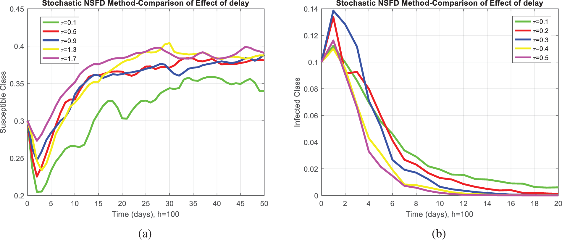
Figure 3: Delay effects plots: (a) The effect of delay of different values on the susceptible class at
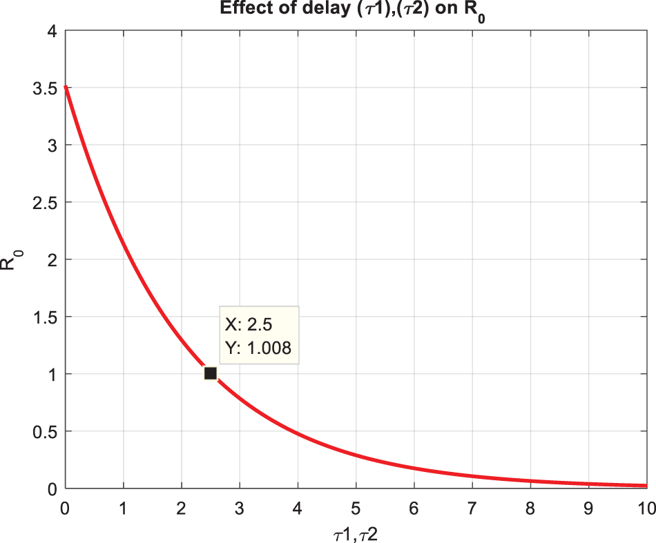
Figure 4: Time plot of the effect of time delay
The study thoroughly evaluates the mathematical analysis of delayed epidemic models for meningitis using reliable delay approaches. Subpopulations are divided by the model into four categories: susceptible, carrier, infected, and recovered. The model’s equilibria, feasible region, and reproduction number are investigated rigorously. After that, two techniques, transition probabilities, and non-parametric perturbation, are implemented successfully on the existing deterministic model of meningitis bacterial disease in the sense of delay effect. The critical points of the newly stochastic version of the model, such as positivity, boundedness, extinction (means on which condition disease will become extinct from the population), and persistence (means on which condition disease will persist in the population), are studied in support of theorems. The Euler Maruyama, stochastic Euler, and stochastic Runge Kutta methods are successfully implemented on both stochastic versions of the model. Unfortunately, as observed in a comparison section, these methods have many discrepancies, such as negative, unbounded, and inconsistent results, and even work for a short period. The nonstandard computation method is implemented on the non-parametric version of the deterministic model to overcome these discrepancies. In this study, the proposed method ensures the biological properties of real-world problems. The most effective, efficient, and precise technique is the nonstandard computational method with stochastic in the sense of delay. In addition, the local and global stabilities of nonstandard computational methods are studied rigorously around the equilibria of the model using the Lyapunov theory after assuming the perturbation is zero. Accordingly, the nonstandard computation method with delay and stochastic is a good agreement for studying such complex models, and their results are close to nature by fulfilling the biological properties of the model.
Acknowledgement: All authors are grateful for the valuable comments of anonymous reviewers. Furthermore, all authors reviewed the results and approved the final version of the manuscript. The authors extend their appreciation to the Deanship of Research and Graduate Studies at King Khalid University for funding this work through Large Research Project under Grant Number RGP2 /302/45. Also, this work was supported by the Deanship of Scientific Research, Vice Presidency for Graduate Studies and Scientific Research, King Faisal University, Saudi Arabia (Grant Number A426).
Funding Statement: The authors extend their appreciation to the Deanship of Research and Graduate Studies at King Khalid University for funding this work through large Research Project under Grant Number RGP2 /302/45. Also, this work was supported by the Deanship of Scientific Research, Vice Presidency for Graduate Studies and Scientific Research, King Faisal University, Saudi Arabia (Grant Number A426).
Author Contributions: Ali Raza: Conceptualization, Investigation, Data curation, Writing—original draft. Mohamed Mahyoub Al-Shamiri: Project administration, Conceptualization, Investigation, Funding acquisition. Emad Fadhal: Data curation, Resources, Investigation, Funding acquisition. Muhammad Rafiq and Nauman Ahmed: Resources, Supervision, Project administration. Umar Shafique: Software, Writing—original draft & review & editing. All authors reviewed the results and approved the final version of the manuscript.
Availability of Data and Materials: All the data used and analyzed is available in the manuscript.
Ethics Approval: Not applicable.
Conflicts of Interest: The authors declare that they have no conflicts of interest to report regarding the present study.
References
1. Kim KS. Acute bacterial meningitis in infants and children. Lancet Infect Dis. 2010;10(1):32–42. doi:10.1016/S1473-3099(09)70306-8. [Google Scholar] [PubMed] [CrossRef]
2. Shin SH, Kim KS. Treatment of bacterial meningitis: an update. Expert Opin Pharmacother. 2012;13(15):2189–206. doi:10.1517/14656566.2012.724399. [Google Scholar] [PubMed] [CrossRef]
3. Madaki UY, Shuaibu A, Umar MI. A mathematical model for the dynamics of bacterial meningitis (Meningococcal meningitisa case study of Yobe State Specialist Hospital, Damaturu, Nigeria. Gadau J Pure Appl Sci. 2023;2(2):113–29. doi:10.54117/gjpas.v2i2.19. [Google Scholar] [CrossRef]
4. Klein M, Abdel-Hadi C, Bühler R, Grabein B, Linn J, Nau R, et al. German guidelines on community-acquired acute bacterial meningitis in adults. Neurol Res Pract. 2023;5(1):01–11. doi:10.1186/s42466-023-00264-6. [Google Scholar] [PubMed] [CrossRef]
5. Chazuka Z, Madubueze CE, Chukwu CW, Chikuni SM. Stability analysis of a bacterial meningitis model with saturated incidence and treatment default. Math Models Comput Simul. 2023;15(2):323–37. doi:10.1134/S2070048223020187. [Google Scholar] [CrossRef]
6. Crankson MV, Olotu O, Afolabi AS, Abidemi A. Modeling the vaccination control of bacterial meningitis transmission dynamics: a case study. Math Model Control. 2023;3(4):416–34. doi:10.3934/mmc.2023033. [Google Scholar] [CrossRef]
7. Turkun C, Golgeli M, Atay FM. A mathematical interpretation for outbreaks of bacterial meningitis under the effect of time-dependent transmission parameters. Nonlinear Dyn. 2023;12(2):01–18. [Google Scholar]
8. Mohanty S, Kostenniemi UJ, Silfverdal SA, Salomonsson S, Iovino F, Sarpong EM et al. Increased risk of long-term disabilities following childhood bacterial meningitis in Sweden. JAMA Netw Open. 2024;7(1):402–15. doi:10.1001/jamanetworkopen.2023.52402. [Google Scholar] [PubMed] [CrossRef]
9. Van RN, Tubiana S, Broucker T, Cedric J, Roy C, Meyohas MC, et al. Persistent headaches one year after bacterial meningitis: prevalence, determinants, and impact on quality of life. Eur J Clin Microbiol Infect Dis. 2023;42(12):1459–67. doi:10.1007/s10096-023-04673-y. [Google Scholar] [PubMed] [CrossRef]
10. Rauti R, Navok S, Biran D, Tadmor K, Leichtmann-Bardoogo Y, Ron EZ, et al. Insight on bacterial newborn meningitis using a neurovascular-unit-on-a-chip. Microbiol Spectr. 2023;11(3):e0123323. doi:10.1128/spectrum.01233-23. [Google Scholar] [PubMed] [CrossRef]
11. Hou Y, Zhang M, Jiang Q, Yang Y, Liu J, Yuan K, et al. Microbial signatures of neonatal bacterial meningitis from multiple body sites. Front Cell Infect Microbiol. 2023;13:1169101. doi:10.3389/fcimb.2023.1169101. [Google Scholar] [PubMed] [CrossRef]
12. Signing F, Tsanou B, Lubuma J, Bowong S. Effects of periodic aerosol emission on the transmission dynamics of neisseria meningitis A. Math Comput Simul. 2023;204(3):43–70. doi:10.1016/j.matcom.2022.06.005. [Google Scholar] [CrossRef]
13. Afridi JK, Karim R, Idrees M, Yar S, Lala G, Gul H. Assessment of neonatal meningitis in a unique presentation with sepsis. J Postgrad Med Inst. 2023;37(2):130–34. [Google Scholar]
14. Buonomo B, Marca RD. A behavioural vaccination model with application to meningitis spread in Nigeria. Appl Math Model. 2024;125(2):334–50. doi:10.1016/j.apm.2023.09.031. [Google Scholar] [CrossRef]
15. Babatunde RS, Adigun O, Folasade O. Towards prediction of cerebrospinal meningitis disease occurrence using logistics regression-a web-based application. FUDMA J Sci. 2023;7(4):337–43. doi:10.33003/fjs-2023-0704-1957. [Google Scholar] [CrossRef]
16. Bradley JS, Bulitta JB, Cook R, Yu PA, Iwamoto C, Hesse EM, et al. Central nervous system antimicrobial exposure and proposed dosing for anthrax meningitis. Clin Infect Dis. 2024;78(6):01–18. doi:10.1093/cid/ciae093. [Google Scholar] [PubMed] [CrossRef]
17. Choi BK, Choi YJ, Sung M, Ha W, Chu MK, Kim WJ, et al. Development and validation of an artificial intelligence model for the early classification of the aetiology of meningitis and encephalitis: a retrospective observational study. Clin Med. 2023;61:34–45. doi:10.1016/j.eclinm.2023.102051. [Google Scholar] [PubMed] [CrossRef]
18. Chen Y, Luo C, Zhou G, Wang H, Dai K, Wu W, et al. The discrimination between autoimmune glial fibrillary acidic protein astrocytopathy and tuberculous meningitis. Mult Scler Relat Disord. 2024;6(1):105527–32. doi:10.1016/j.msard.2024.105527. [Google Scholar] [PubMed] [CrossRef]
19. Olu OT, Michael OO, Nathaniel OS, Abraham OA, Emmanuel FS, James AK, et al. Propagation dynamics of meningitis disease based on complex network modeling. Univ J Public Health. 2023;11(3):324–31. doi:10.13189/ujph.2023.110306. [Google Scholar] [CrossRef]
20. Ahmad H, Khan TA, Ahmad I, Stanimirovic PS, Chu YM. A new analyzing technique for nonlinear time fractional Cauchy reaction-diffusion model equations. Results Phys. 2020;19:103462. doi:10.1016/j.rinp.2020.103462. [Google Scholar] [CrossRef]
21. Enatsu Y, Nakata Y, Muroya Y, Izzo G, Vecchio A. Global dynamics of difference equations for SIR epidemic models with a class of nonlinear incidence rates. J Differ Equ Appl. 2012;18(7):1163–81. doi:10.1080/10236198.2011.555405. [Google Scholar] [CrossRef]
Cite This Article
 Copyright © 2024 The Author(s). Published by Tech Science Press.
This work is licensed under a Creative Commons Attribution 4.0 International License , which permits unrestricted use, distribution, and reproduction in any medium, provided the original work is properly cited.
 Downloads
 Citation Tools