
 Submit a Paper
 Propose a Special lssue
 Open Access
ARTICLE

A Hermitian C Differential Reproducing Kernel Interpolation Meshless Method for the 3D Microstructure-Dependent Static Flexural Analysis of Simply Supported and Functionally Graded Microplates
Department of Civil Engineering, National Cheng Kung University, Tainan, 70101, Taiwan
* Corresponding Author: Chih-Ping Wu. Email:
(This article belongs to the Special Issue: Theoretical and Computational Modeling of Advanced Materials and Structures-II)
Computer Modeling in Engineering & Sciences 2024, 141(1), 917-949. https://doi.org/10.32604/cmes.2024.052307
Received 29 March 2024; Accepted 21 June 2024; Issue published 20 August 2024
 View Full Text
 Download PDF
Abstract
This work develops a Hermitian C differential reproducing kernel interpolation meshless (DRKIM) method within the consistent couple stress theory (CCST) framework to study the three-dimensional (3D) microstructure-dependent static flexural behavior of a functionally graded (FG) microplate subjected to mechanical loads and placed under full simple supports. In the formulation, we select the transverse stress and displacement components and their first- and second-order derivatives as primary variables. Then, we set up the differential reproducing conditions (DRCs) to obtain the shape functions of the Hermitian C differential reproducing kernel (DRK) interpolant’s derivatives without using direct differentiation. The interpolant’s shape function is combined with a primitive function that possesses Kronecker delta properties and an enrichment function that constituents DRCs. As a result, the primary variables and their first- and second-order derivatives satisfy the nodal interpolation properties. Subsequently, incorporating our Hermitian C DRK interpolant into the strong form of the 3D CCST, we develop a DRKIM method to analyze the FG microplate’s 3D microstructure-dependent static flexural behavior. The Hermitian C DRKIM method is confirmed to be accurate and fast in its convergence rate by comparing the solutions it produces with the relevant 3D solutions available in the literature. Finally, the impact of essential factors on the transverse stresses, in-plane stresses, displacements, and couple stresses that are induced in the loaded microplate is examined. These factors include the length-to-thickness ratio, the material length-scale parameter, and the inhomogeneity index, which appear to be significant.Keywords
With the increasing demand for microstructures in industry and the rapid progress in material manufacturing technology, functionally graded (FG) structures have gradually shrunk from the macro scale to the micron scale. FG microstructures are gradually being used in cutting-edge technology fields, including thin films [1,2], micro-electro-mechanical systems [3,4], and atomic force microscopes [5,6]. Thus, developing an effective computational method to investigate the mechanical behavior of these microstructures has attracted considerable attention.
It is well-known that the mechanical behavior of FG macrostructures will be changed as their dimensions shrink from the macro-scale to the micro-scale [7]. The existing shell, plate, and beam theories based on the classical continuum mechanics (CCM) are inappropriate for use to analyze the dynamic and static responses of FG microshells, microplates, and microbeams due to the microstructure-dependent effect becoming significant. As a result, some non-CCM-based theoretical methods accounting for the microstructure-dependent impact have been proposed to investigate the mechanical behavior of microstructures. These theoretical methods include the couple stress theory (CST) [8,9], the strain gradient theory (SGT) [10,11], the doublet mechanics theory [12], the micropolar elasticity theory [13,14], and the nonlocal elasticity theory [15].
Hadjesfandiari et al. [16,17] and Yang et al. [18] established the consistent CST (CCST) and the modified CST (MCST) by assuming the couple-stress tensor is skew-symmetric and symmetric, respectively. As a result, instead of two material length-scale coefficients, which are required to study an elastic isotropic body’s mechanical behavior when the original CST is employed, only one material length-scale coefficient is needed when the MCST/CCST is employed. This facilitates their future application.
Within the CCST/MCST framework, some two-dimensional (2D) shear deformation theories for investigating the microstructure-dependent mechanical behavior of FG microplates/microshells have been developed by assuming particular kinematics models a priori. Beni et al. [19] presented a microstructure-dependent classical shell theory on the basis of the MCST to determine an FG circular cylindrical microshell’s smallest natural frequency and its corresponding wave number pair. Incorporating Mindlin’s kinematics model into the MCST, Ma et al. [20] established a microstructure-dependent first-order shear deformation theory (FOSDT) to analyze a homogeneous isotropic microplate’s flexural and free vibration behaviors. Arefi et al. [21] developed a novel shear deformation theory on the basis of the MCST to examine a three-layered microplate’s stress and displacement, for which the microplate of interest consists of an exponentially graded (EG) core and two piezomagnetic face sheets. Based on Hamilton’s principle combined with Reddy’s kinematics model, Lei et al. [22] and Thai et al. [23] presented a microstructure-dependent refined shear deformation theory (RSDT) on the basis of the MCST to conduct an FG microplate’s microstructure-dependent deformation and natural frequency behavior analyses. Kim et al. [24] developed a microstructure-dependent and MCSD-based third-order shear deformation theory (TOSDT) to investigate an FG microplate’s static buckling, static flexural, and free vibration behaviors. Thai et al. [25] developed a microstructure-dependent sinusoidal shear deformation theory (SSDT) on the basis of the MCST to examine an FG microplate’s static flexural and free vibration behaviors. Sobhy et al. [26] presented a microstructure-dependent and MCST-based trigonometric shear deformation theory (TSDT) with four primary variables for modeling an EG microplate’s static buckling, static flexural, and free vibration characteristics resting on Pasternak’s foundation.
Unlike these 2D microstructure-dependent and MCST-based shear deformation theories mentioned above, Wu et al. [27] established the unified microstructure-dependent shear deformation theories based on the CCST to study an FG/EG elastic microplate’s mechanical behavior. Their results showed that the CCST and MCST solutions of deformation and natural frequency associated with out-of-plane vibration modes are almost identical when setting the value of MCST’s material length-scale parameter at twice that of CCST’s material length-scale parameter. However, their solutions of natural frequency associated with the in-plane vibration modes are slightly different.
Instead of the CCST and MCST, other non-CCM-based analytical and numerical methods, including the SGT, the differential quadrature method (DQM), the iso-geometric analysis technique (IGAT), etc., have also been employed to study an FG microplate’s mechanical behavior. Incorporating Kirchhoff-Love’s kinematics model into the SGT, Deng et al. [28] established a non-CCM-based theory to determine an FG microplate’s smallest natural frequency with variable thickness. Within the SGT framework, Balobanov et al. [29] presented a microstructure-dependent classical thin shell theory to investigate a circular cylindrical microscale shell’s static flexural behavior. Integrating the advantages of the finite element method (FEM) and the DQM, Zhang et al. [30] developed a Hermitian C1 four-node quadrilateral element for conducting a moderately thick microplate’s mechanical behavior analysis. Integrating the MCST and the IGAT, Thanh et al. [31] established a seventh-order shear deformation theory for analyzing a porous FG microplate’s microstructure-dependent nonlinear thermal stability behavior. Nguyen et al. [32] developed a computational approach for analyzing an FG microplate’s geometrically nonlinear behavior on the basis of the IGAT and the RSDT. In conjunction with a modified nonlocal CST and the IGAT, Pham et al. [33] conducted an FG microplate’s static flexural and free vibration characteristics analyses, where the microplate rested on an elastic foundation. Based on the CCST, Wu and his colleagues [34,35] established a semi-analytical Hermitian Cn FEM to conduct elastic and piezoelectric microscale plates’/shells’ microstructure-dependent static and dynamic behavior analyses.
Meshless methods have also been employed to investigate a microscale structure’s mechanical behavior. Incorporating Mindlin’s kinematics model and radial basis functions into the MCST, Roque et al. [36] proposed a point collocation method for analyzing a homogeneous isotropic microplate’s static flexural behavior. Incorporating HSDT’s kinematics model into the MCST, Tran et al. [37] and Thai et al. [38] presented a moving Kriging interpolation meshless method to investigate an FG sandwich microplate’s static buckling, static flexural, and free vibration characteristics. Nguyen et al. [39] incorporated a four-variable kinematics model into the MCST to develop a non-uniform rational B-splines (NURBS) meshless method, which was used to investigate an FG microplate’s microstructure-dependent static buckling, static flexural, and free vibration behaviors. Finally, Thai et al. [40] employed the NURBS meshless method to conduct an FG microplate’s static buckling and free vibration behavior analyses.
In their series of papers, Li et al. [41], Simkins et al. [42], Liu et al. [43], and Lu et al. [44] established the reproducing kernel element method to solve Galerkin weak forms of a system of higher order partial differential equations which are associated with Dirichlet boundary conditions.
Chen et al. [45] and Wang et al. [46] established the Hermitian C1 and Lagrange C0 differential reproducing kernel interpolation meshless (DRKIM) methods, respectively, for investigating laminated composite and FG macroscale structures’ mechanical behavior. The novelty of these DRKIM methods is that the shape functions of the differential reproducing kernel (DRK) interpolant’s derivatives are obtained by setting up the differential reproducing conditions (DRCs) without using direct differentiation, as is necessary for the conventional reproducing kernel interpolation and approximation methods [47]. It has been shown that the solutions obtained using these DRKIM methods closely agree with the available 3D solutions of macroscale plates, rather than those of microplates.
As we see in the strong form of the 3D CCST, the primary variables’ highest order derivative is the third order for microplates, which differs from the first order designation for macroscale plates. This situation will reduce the accuracy of the early proposed Hermitian C1 and Lagrangian C0 DRKIM methods and slow down their convergence rate. To enhance these DRKIM methods’ accuracy and speed up their convergence rate, in this paper, we aim to establish a Hermitian C2 DRKIM method by making some modifications: the Hermitian C2 DRK interpolant should satisfy the nodal interpolation properties and the continuity conditions up to primary variables’ second-order derivatives at each sampling node. Moreover, we also aim to establish the Hermitian C2 DRKIM method, which is a point collocation method, by incorporating our Hermitian C2 DRK interpolant into the strong form of the 3D CCST to carry out an FG microplate’s 3D microstructure-dependent static flexural analysis. After validating the Hermitian C2 DRKIM’s accuracy using the relevant 3D solutions reported in the literature, we will carry out a parametric study for the FG microplate’s 3D microstructure-dependent static flexural behavior to examine how the impact of essential factors affects the induced deformations, in-plane stresses, transverse stresses, and couple stresses, including the length-to-thickness ratio, the material length-scale parameter, and the inhomogeneity index.
2 The Hermitian C2 DRKIM Method
2.1 The Hermitian C2 DRK Interpolant
We consider
where
In order to determine the undetermined function vector
Eq. (5) can be rearranged in the following explicit forms:
We rewrite Eqs. (6)–(9) in matrix form as follows:
where
We substitute the enrichment functions into the DRCs to yield the following expression for the undetermined function vector
where
We substitute Eq. (11) into Eq. (1) to yield the shape functions of the Hermitrian C2 DRK interpolant as follows:
where
Eq. (11) shows that the enrichment functions vanish at all the sampling points (i.e.,
2.2 The Hermitian C2 DRK Interpolant’s Derivatives
The Hermitian C2 DRK interpolant
where
In order to determine the undetermined functions
where
We rearrange Eq. (16) in the explicit forms as follows:
We rewrite the above Eqs. (17)–(20) in matrix form as follows:
where
We substitute the enrichment functions into the DRCs to yield the undetermined function vector
We substitute Eq. (22) into Eq. (15) to obtain the shape functions of the Hermitian C2 DRK interpolant’s first-order derivatives as follows:
where
From Eqs. (23)–(25), it can be seen that the values of the enrichment functions’ first-order derivatives at all sampling nodes are zero (i.e.,
Similarly, the above derivation procedure can proceed to the rth-order derivative of the Hermitian C2 DRK interpolant
2.3 Weight Functions and Primitive Functions
In implementing our Hermitian C2 DRKIM method, we must select the weight function and the primitive function in advance. This work uses the normalized Gaussian function as the weight function, which is expressed as follows [47]:
where
As mentioned above, we define the primitive functions for the Hermitian C2 DRK interpolant as
where
It is noticed that for a meshless method, the support size
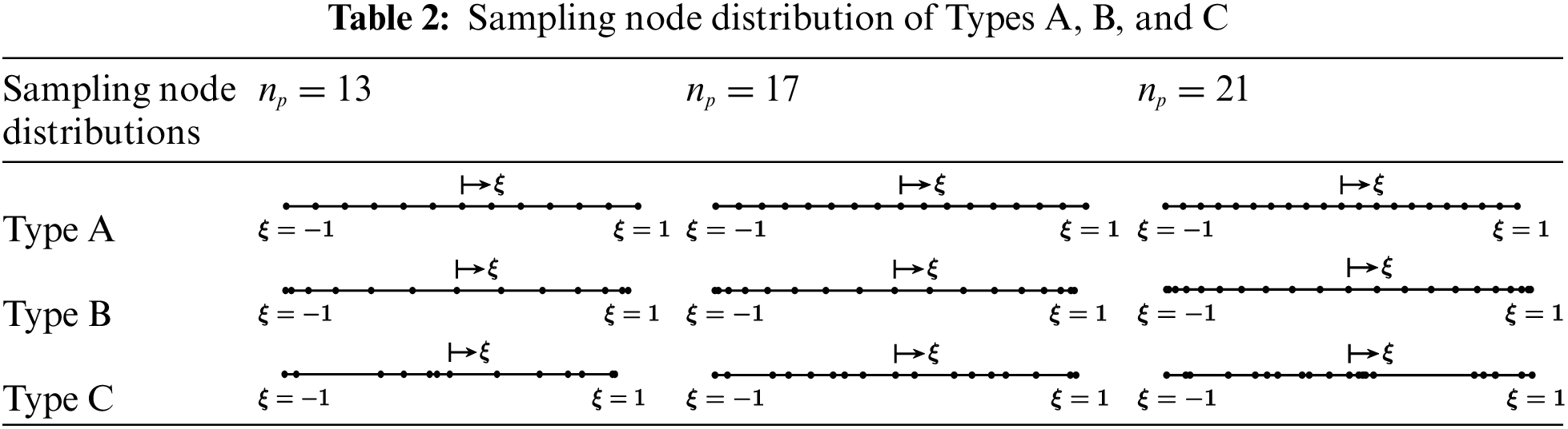
To have a clear picture related to how the values of these shape functions vary in the natural coordinate, in Fig. 1a–c, we consider a case of 11 sampling nodes with uniform spacing and present the distributions of the enrichment function (

Figure 1: Distributions of (a) the enrichment function, (b) the primitive function, and (c) the shape function of node 6 in the natural coordinate in the case of np = 11 with uniform spacing


Figure 2: Distributions of the shape functions (a) (i = 1–3), (b) (i = 4–6), (c) (i = 7–9), and (d) (i = 10 and 11), in the natural coordinate in the case of np = 11 with uniform spacing
3 3D Microstructure-Dependent Static Flexural Analysis of FG/EG Microplates
3.1 The Quasi-State Space Equations of the CCST
This work considers the 3D microstructure-dependent static flexural problem of a simply-supported FG microplate under either a sinusoidally distributed load or a uniform load, and the former loading case is shown in Fig. 3. The symbols h, Lx, and Ly represent the microplate’s height, length, and width, respectively. A Cartesian coordinate system (

Figure 3: An FG microplate of interest that is subjected to a sinusoidally distributed load
The displacement vector u of the deformed microplate is expressed as
The strain tensor
where the commas represent the partial derivative of the suffix variable.
The rotation tensor
The symmetric part of the curvature tensor
The skew-symmetric part of the curvature tensor
Hadjesfandiari and Dargush [16,17] indicated that in general, the force-stress tensor (
The linear constitutive equations for a loaded orthotropic material microplate are given by
where
The stress equilibrium equations of a microplate, following Hadjesfandiari and Dargush’s analysis [16,17], are given by
where as mentioned above,
We employ the direct elimination to reduce the above equations to six partial differential equations which are expressed in terms of six primary variables: three transverse stresses (
Substituting Eqs. (32) and (34) into the fifth equation of Eq. (33) leads to
Substituting Eqs. (32) and (34) into the fourth equation of Eq. (33) leads to
Substituting Eq. (28c) into the third equation of Eq. (33) leads to
where
Using the relationships of
where
Eqs. (38)–(43) represent the quasi-state space equations for the FG microplates’ 3D microstructure-dependent static flexural behavior. In addition, we can reduce these equations for examining FG microscale plates to those for examining FG macroscale plates by letting the value of l zero.
The microplate’s surface and edge boundary conditions are specified in the following forms [16,17]:
On the top and bottom surfaces,
where the positive directions of
For simply supported boundary edges, we express the edge boundary conditions in the following forms:
At the edges
At the edges
3.2 Fourier Series Expansion Method
This work lets the external loads
where the symbols
We also express these primary variables as the following double Fourier series:
Substituting Eqs. (47)–(52) into the quasi-state space Eqs. (38)–(43) yields
3.3 The Hermitian C2 DRKIM Method
This section develops the Hermitian C2 DRKIM method, which is a point collocation, for solving the strong form of the 3D CCST, which is composed of the quasi-state space Eqs. (53)–(58) and their associated boundary conditions (45a) and (45b).
First, we select nc collocation points in the thickness direction, for which nc = 3np, and then substitute the primary variables expressed in Eq. (1) and their relevant derivatives into the quasi-state space Eqs. (53)–(58) at the ith-collocation point, which leads to the following algebraic equations:
where
The associated surface conditions, which are five conditions on the top surface and five conditions on the bottom surface, are given as
As mentioned above, Eqs. (59)–(64) and (65a), (65b) represent a system of (6nc + 10) (i.e., 18np + 10) algebraic equations in terms of 18np nodal primary variables, which can be readily solved employing the weighted least square method.
4.1 Validation and Comparison Studies
This section considers a simply supported FG microplate that is subjected to either a sinusoidally distributed load or a uniform load. The former loading conditions are shown in Fig. 3.
The microplate of interest is made of alumina (Al2O3, a ceramic material) and aluminum (Al, a metal material). The microplate’s material properties are assumed to obey the power-law distributions for the constituents’ volume fractions, which vary in the thickness direction and are defined as follows:
and
where the subscripts cer and met denote the ceramic and metal materials, respectively.
The material properties of the alumina and the aluminum are given in the following form [23]:
For aluminum material,
By using the rule of mixtures, we estimate the microplate’s effective material properties as follows:
For comparison purposes, we define the non-dimensional variables in the same way as those used in Thai et al. [23]:
When considering a homogeneous isotropic microplate, we change Ecer in Eq. (69a) to the microplate’s Young’s modulus, E0.
According to Lam et al.’s experimental results [7], this work defines the material length-scale parameters of the MCST and the CCST,
Table 1 shows the results of the Hermitian C2 DRK meshless method for the central deflection
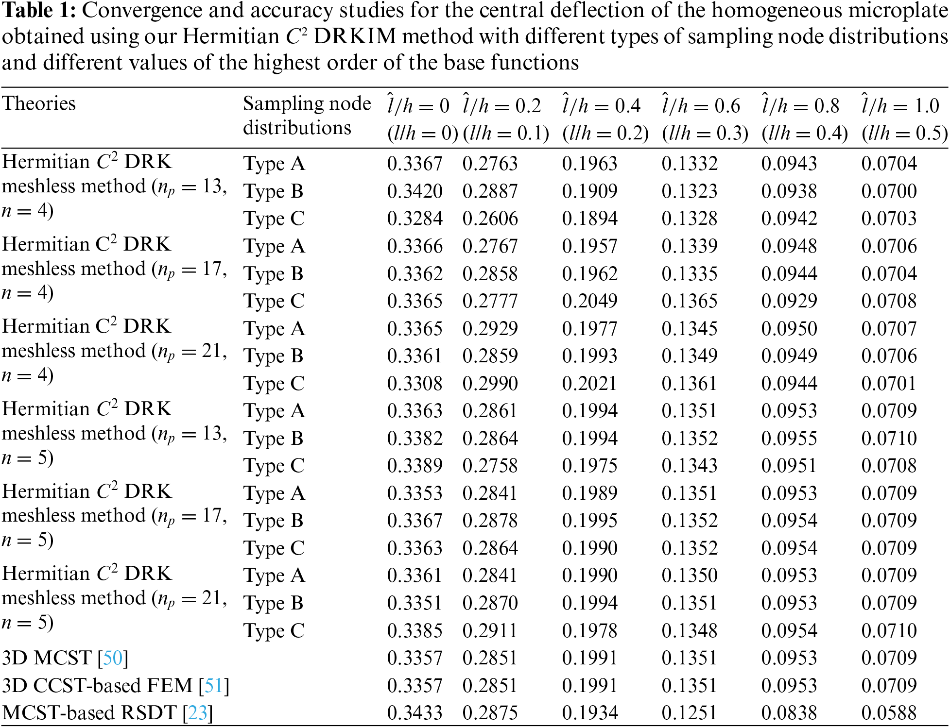
Compared with the 3D solutions [50,51], Table 1 shows that the solutions obtained using our Hermitian C2 DRKIM method with n = 5 are more accurate than those with n = 4. The solutions obtained using the Hermitian C2 DRKIM method with the sampling node distributions of Types A and B are more precise than those with Type C sampling node distributions. For a range of the values of the l/h ratio from l/h = 0 to l/h = 0.5, the maximum relative error between the solutions obtained using the Hermitian C2 DRKIM method and those obtained using the 3D MCST [50] is 0.35% and 0.67% for Type A and Type B sampling node distributions, respectively. The relative error between the solutions obtained using 3D MCST and the 2D RSDT [23] is 2.3% in the case of l/h = 0, and it increases up to 17.1% in the case of l/h = 0.5. This is because the 3D couple stress effect is significant when the value of the l/h ratio increases. Because our Hermitian C2 DRKIM method is based on the strong form of the 3D CCST, its performance is superior to that of the 2D MCST-based microplate theory, especially for the microplates with a higher value of the l/h ratio.
Table 3 shows accuracy studies for the central deflection results of a simply supported homogeneous microplate obtained using our Hermitian C2 DRKIM method with a uniform node distribution (i.e., Type A) and different values of the support size al and the l/h ratio. The microplate considered here is subjected to the same loads as used in Table 1. The relevant parameters are
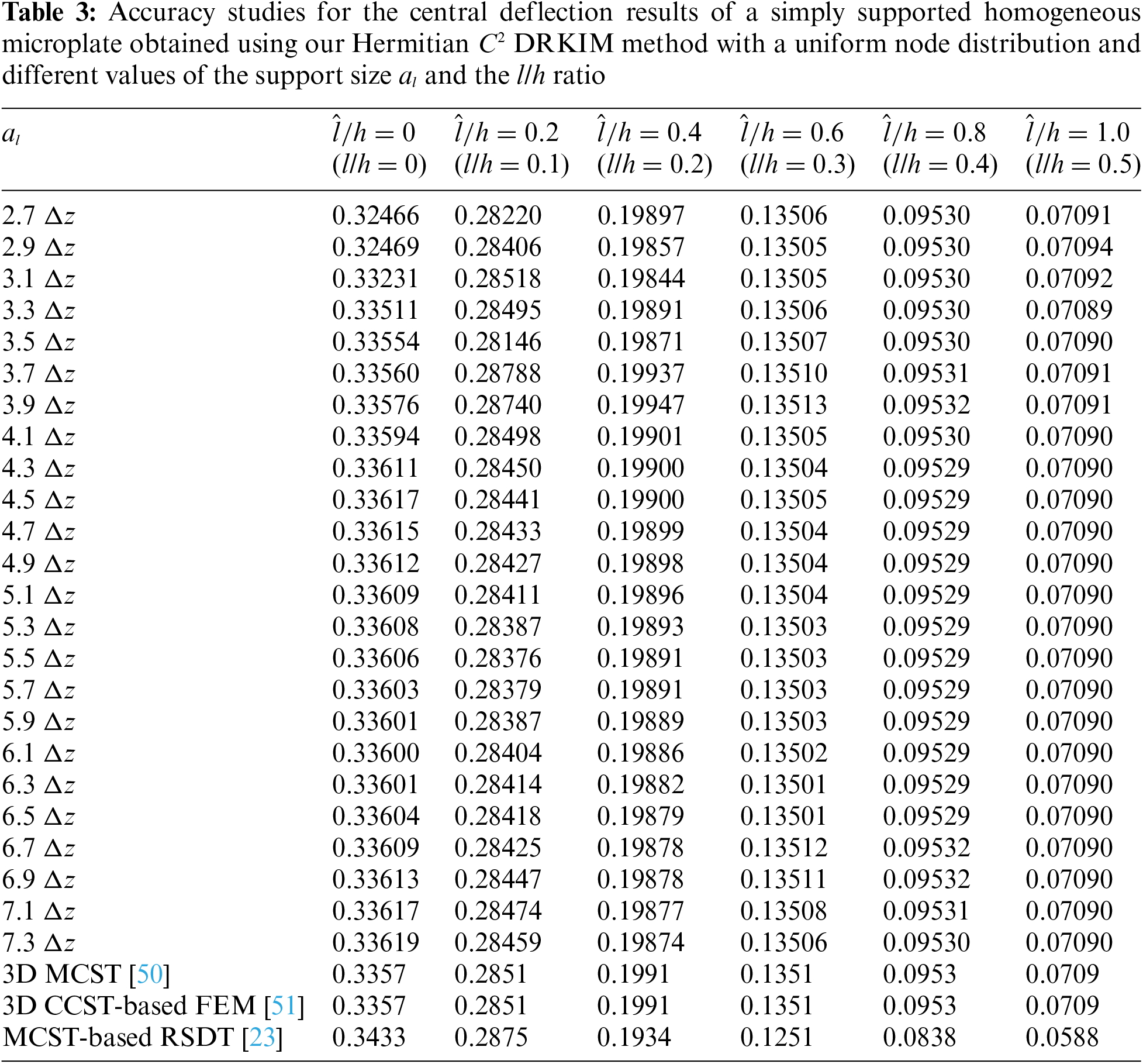
Table 4 shows that the comparisons of the central deflection results of a simply-supported FG microplate obtained using our Hermitian C2 DRKIM method with np = 31 and n = 5, the 3D CCST-based FEM [51], the refined quasi-3D IGAT [39], the MCST- and CCST-based RSDTs [23,27], and the CCST-based CPT [27]. The relevant geometric parameters are given as Lx/h = 5 and 20 and

The loading conditions considered here are sinusoidally distributed loads and uniform loads and are expressed as follows:
For the sinusoidal type load,
For the uniform-type load,
where in the following analysis, the convergent solutions are yielded when the values of
As previously mentioned, the microplate is made of Al2O3 and Al materials, and their volume fractions are given in Eqs. (66a) and (66b). Table 4 shows the Hermitian C2 DRKIM method’s results closely agree with those obtained using the 3D CCST-based FEM [51] and the quasi-3D IGAT [39]. It can be seen in Table 4 that the FG microplate’s central deflection decreases when the value of the material length-scale parameter rises, indicating that an increase in the material length-scale parameter stiffens the microscale plate, decreasing its central deflection. The central deflection increases when the value of the inhomogeneity index (
Table 5 shows the comparisons for the results of the FG microplate’s in-plane stresses and deflections obtained using various 2D microstructure-dependent shear deformation theories on the basis of the MCST/CCST and our Hermitian C2 DRKIM method. The relevant material parameters are

This section presents a parametric study to understand the impact of essential factors on deformations, in-plane stresses, transverse stresses, and couple stresses induced in an EG microplate, which is placed under full simple supports and is subjected to mechanical loads. The microplate considered here is subjected to the sinusoidally distributed loads, which are
where Eb = 70 Gpa. When
The dimensionless variables used in the following study are given as
It is important to note that using dimensionless variables in the following analysis allows for a more comprehensive understanding of the results. For instance, when the value of the l/h ratio is fixed, like l/h = d, as we change the value of l and let h = l/d, or we change the value of h and let l = (hd), we always obtain the same results. This approach enhances the robustness and applicability of our findings.
Fig. 4a–h shows the variations in dimensionless displacements, in-plane stresses, transverse stresses, and couple stresses induced in an EG microplate along the thickness direction, with the values of the inhomogeneity index (


Figure 4: Variations in the dimensionless (a) in-plane displacement
Fig. 5a–h shows the variations in the dimensionless displacement, in-plane stresses, transverse stresses, and couple stresses induced in an EG microplate along the thickness direction, with the values of the l/h ratio being 0, 0.2, and 0.4. The other material parameter is


Figure 5: Variations in the dimensionless (a) in-plane displacement
It can be seen in Fig. 5b that an increase in the value of l stiffens the microplate, leading to its deflection decrease. The results in Fig. 5c–f show that the variations in the in-plane stress and transverse stress induced in the microplate along its thickness direction with a smaller value of l are more significant than those induced in the microplate along the thickness direction with a more considerable value of l. This is because an increase in the value of l stiffens the microplate, which leads to fewer deformations and fewer stresses induced in the microplate when the magnitude of the applied load remains constant. The results in Fig. 5g and h show that the variations in the couple stresses (
Fig. 6a–h shows that the variations in the dimensionless deformations, in-plane stresses, transverse stresses, and couple stresses induced in an EG microplate along the thickness direction, with the length-to-thickness ratios being 5, 10, and 20. The relevant material parameters are l/h = 0.5 and

Figure 6: Variations in the dimensionless (a) in-plane displacement
5 Concluding Remarks
A Hermitian C2 DRKIM method based on the strong form of the 3D CCST has been developed for analyzing the 3D microstructure-dependent static flexural behavior of an FG/EG microplate. The FG/EG microplate considered here was subjected to mechanical loads and placed under full simple supports. The unique features of this Hermitian C2 DRK interpolant compared with the early Lagrange-type reproducing kernel interpolant for analyzing macroscale plate’s mechanical behavior are that the displacements, the transverse stresses, and their first-order and second-order derivatives are selected as primary variables satisfying the nodal interpolation properties, and their corresponding shape functions satisfy the Kronecker delta properties. These features make our Hermitian C2 DRKIM method suitable for analyzing the FG microplate’s mechanical behavior because the deflections and rotations prescribed at the boundary edges of the microplate considered here can thus be directly imposed without using the penalty method, which is necessary for the conventional reproducing kernel point collocation method. In addition, using our Hermitian C2 DRKIM method, the primary variables’ higher-order derivatives involved in the strong form of the CCST can be effectively estimated.
In the validation and comparison study, the solutions obtained using our Hermitian C2 DRKIM method closely agree with the available 3D solutions in the literature, with a fast convergence rate. Because the 3D couple stress effect is significant when the value of the l/h ratio rises, the performance of the Hermitian C2 DRKIM method is superior to that of 2D CCST-/MCST-based shear deformation microplate theories, especially for the microplate with a considerable value of the l/h ratio. For example, the maximum relative error between the solutions obtained using the Hermitian C2 DRKIM method and those obtained using the 3D MCST is 0.35% for a range of the value of the l/h ratio between l/h = 0 and l/h = 0.5, respectively; however, the relative error between the solutions obtained using the 2D RSDT and the 3D MCST solutions is 2.3% in the case of l/h = 0, and it increases up to 17.1% when the value of the l/h ratio is 0.5.
In the parametric study, we presented the displacement, in-plane stress, transverse stress, and couple stress distributions along the thickness direction of an EG microplate using our Hermitian C2 DRKIM method. These distributions cannot be effectively estimated using existing 2D microstructure-dependent shear deformation theories, especially for the transverse stress and couple stress distributions, so they have yet to be shown in public literature. Thus, the parametric analysis results can provide a reference for assessing the accuracy of existing 2D microstructure-dependent shear deformation theories. Furthermore, the results are also helpful for making assumptions about primary variable components for an advanced microstructure-dependent shear deformation microplate theory, which is to be developed.
Acknowledgement: The authors thank the National Science and Technology Council of the Republic of China for its financial support.
Funding Statement: This study was supported by a grant from the National Science and Technology Council, Taiwan (Grant Number: MOST 112-2221-E-006-048-MY2).
Author Contributions: Chih-Ping Wu: Conceptualization, Methodology, Validation, Formal analysis, Investigation, Resources, Data curation, Writing—original draft preparation, Writing—review and editing, Supervision, Project administration, Funding acquisition. Ruei-Syuan Chang: Software, Validation, Formal analysis, Investigation, Data curation. All authors reviewed the results and approved the final version of the manuscript.
Availability of Data and Materials: The processed data required to reproduce these findings can be downloaded from https://docs.google.com/document/d/1hvfVYcF5hsGj-4HEn4WOJL9y3hNq68Q/edit?usp=drive_link&ouid=103032847656566806520&rtpof=true&sd=true (accessed on 20 May 2024).
Conflicts of Interest: The authors declare they have no conflicts of interest to report regarding the current study.
References
1. Hossain MI, Masour S. A critical overview of thin films coating technologies for energy applications. Cogent Eng. 2023;10(1):2179467. [Google Scholar]
2. Sathish M, Radhika N. Current status, challenges, and future prospects of thin film costing techniques and coating structures. J Bio Tribo Corros. 2023;9:35. [Google Scholar]
3. Faudzi AAM, Sabzehmeidani Y, Suzumori K. Application of micro-electro-mechanical systems (MEMS) as sensors: a review. J Robot Mechatron. 2020;32(2):281–8. [Google Scholar]
4. Gilewski M. Micro-electro-mechanical systems in light stabilization. Sensors. 2023;23(6):2916. [Google Scholar] [PubMed]
5. Magazzu A, Marcuello C. Investigation of soft matter nanomechanics by atomic force microscopy and optical tweezers: a comprehensive review. Nanomater. 2023;13(6):963. [Google Scholar]
6. Liu Q, Fu Y, Qin Z, Wang Y, Zhang S, Ran M. Progress in the applications of atomic force microscope (AFM) for mineralogical research. Micro. 2023;170(1–3):103460. doi:10.1016/j.micron.2023.103460. [Google Scholar] [PubMed] [CrossRef]
7. Lam DCC, Yang F, Chong ACM, Wang J, Tong P. Experiments and theory in strain gradient elasticity. J Mech Phys Solids. 2002;51(8):1477–508. doi:10.1016/S0022-5096(03)00053-X. [Google Scholar] [CrossRef]
8. Soldatos KP. New trends in couple stress hyperelasticity. Math Mech Solids. 2023;67:108128652311776. doi:10.1177/10812865231177673. [Google Scholar] [CrossRef]
9. Taghizadeh M, Babaei M, Dimitri R, Tornabene F. Assessment of critical buckling load of bi-directional functionally graded truncated conical micro-shells using modified couple stress theory and Ritz method. Mech Based Des Struct Mach. 2023;52(6):3456–87. doi:10.1080/15397734.2023.2202230. [Google Scholar] [CrossRef]
10. Zhang Y, Cheng Z, Zhu T, Lu L. Mechanics of gradient nanostructured metals. J Mech Phys Solids. 2024;189:105719. doi:10.1016/j.jmps.2024.105719. [Google Scholar] [CrossRef]
11. Jiang Y, Li L, Hu Y. Strain gradient elasticity theory of polymer networks. Acta Mech. 2022;233:3213–31. [Google Scholar]
12. Ferrari M, Granik VT, Imam A, Nadeau JC. Advances in doublet mechanics. Germany: Springer; 1997. p. 1–26. [Google Scholar]
13. Carrera E, Zozulya VV. Carrera unified formulation (CUF) for the micropolar plates and shells. I. Higher order theory. Mech Adv Mater Struct. 2020;29(6):773–95. [Google Scholar]
14. Carrera E, Zozulya VV. Carrera unified formulation (CUF) for the micropolar plates and shells. II. Complete linear expansion case. Mech Adv Mater Struct. 2020;29(6):796–815. [Google Scholar]
15. Eringen AC. Nonlocal continuum field theories. New York: Springer; 2002. p. 71–176. [Google Scholar]
16. Hadjesfandiari AR, Dargush GF. Couple stress theory for solids. Int J Solids Struct. 2011;48(18):2496–510. [Google Scholar]
17. Hadjesfandiari AR, Dargush GF. Fundamental solutions for isotropic size-dependent couple stress elasticity. Int J Solids Struct. 2013;50(9):1253–65. [Google Scholar]
18. Yang F, Chong ACM, Lam DCC, Tong P. Couple stress-based strain gradient theory for elasticity. Int J Solids Struct. 2002;39(10):2731–43. doi:10.1016/S0020-7683(02)00152-X. [Google Scholar] [CrossRef]
19. Beni YT, Mehralian F, Zeighampour H. The modified couple stress functionally graded cylindrical thin shell formulation. Mech Adv Mater Struct. 2016;23(7):791–801. doi:10.1080/15376494.2015.1029167. [Google Scholar] [CrossRef]
20. Ma HM, Gao XL, Reddy JN. A non-classical Mindlin plate model based on a modified couple stress theory. Acta Mech. 2011;220(1-4):217–35. doi:10.1007/s00707-011-0480-4. [Google Scholar] [CrossRef]
21. Arefi M, Kiani M. Magneto-electro-mechanical bending analysis of three-layered exponentially graded microplate with piezomagnetic face sheets resting on Pasternak’s foundation via MCST. Mech Adv Mater Struct. 2020;27(5):383–95. doi:10.1080/15376494.2018.1473538. [Google Scholar] [CrossRef]
22. Lei J, He Y, Zhang B, Liu D, Shen L, Guo S. A size-dependent FG micro-plate model incorporating higher-order shear and normal deformation effects based on a modified couple stress theory. Int J Mech Sci. 2015;104(5):8–23. doi:10.1016/j.ijmecsci.2015.09.016. [Google Scholar] [CrossRef]
23. Thai HT, Kim SE. A size-dependent functionally graded Reddy plate model based on a modified couple stress theory. Compos Part B. 2013;45(1):1636–45. doi:10.1016/j.compositesb.2012.09.065. [Google Scholar] [CrossRef]
24. Kim J, Reddy JN. Analytical solutions for bending, vibration, and buckling of FGM plates using a couple stress-based third-order theory. Compos Struct. 2013;103(3):86–98. doi:10.1016/j.compstruct.2013.03.007. [Google Scholar] [CrossRef]
25. Thai HT, Vo TP. A size-dependent functionally graded sinusoidal plate model based on a modified couple stress theory. Compos Struct. 2013;96(20):376–83. doi:10.1016/j.compstruct.2012.09.025. [Google Scholar] [CrossRef]
26. Sobhy M, Zenkour AM. A comprehensive study on the size-dependent hygrothermal analysis of exponentially graded microplates on elastic foundations. Mech Adv Mater Struct. 2020;27(10):816–30. doi:10.1080/15376494.2018.1499986. [Google Scholar] [CrossRef]
27. Wu CP, Hu HX. A unified size-dependent plate theory for static bending and free vibration analyses of micro- and nano-scale plates based on the consistent couple stress theory. Mech Mater. 2021;162:104085. doi:10.1016/j.mechmat.2021.104085. [Google Scholar] [CrossRef]
28. Deng T, Zhang B, Liu J, Shen H, Zhang X. Vibration frequency and mode localization characteristics of strain gradient variable-thickness microplates. Thin-Walled Struct. 2024;199:111779. [Google Scholar]
29. Balobanov V, Kiendl J, Khakalo S, Niiranen J. Kirchhoff-Love shells within strain gradient elasticity: weak and strong formulations and an H3-conforming isogeometric implementation. Comput Methods Appl Mech Eng. 2019;344:837–57. [Google Scholar]
30. Zhang B, Li H, Kong L, Zhang X, Feng Z. Strain gradient differential quadrature finite element for moderately thick micro-plates. Int J Numer Methods Eng. 2020;121(24):5600–46. [Google Scholar]
31. Thanh GE, Tran LV, Bui TQ, Nguyen HX, Abdel-Wahab M. Isogeometric analysis for size-dependent nonlinear thermal stability of porous FG microplates. Compos Struct. 2019;221:110838. [Google Scholar]
32. Nguyen NX, Atroshchenko E, Nguyen-Xuan H, Vo TP. Geometrically nonlinear isogeometric analysis of functionally graded microplates with the modified couple stress theory. Comput Struct. 2017;193:110–27. [Google Scholar]
33. Pham QH, Nguyen PC, Tran VK, Lieu QX, Tran TT. Modified nonlocal couple stress isogeometric approach for bending and free vibration analysis of functionally graded nanoplates. Eng Comput. 2023;39(1):993–1018. doi:10.1007/s00366-022-01726-2. [Google Scholar] [CrossRef]
34. Wu CP, Tan TF, Hsu HT. A size-dependent finite element method for the 3D free vibration analysis of functionally graded graphene platelets-reinforced composite cylindrical microshells based on the consistent couple stress theory. Materials. 2023;16(6):2363. doi:10.3390/ma16062363. [Google Scholar] [PubMed] [CrossRef]
35. Wu CP, Wu ML, Hsu HT. 3D size-dependent dynamic instability analysis of FG cylindrical microshells subjected to combinations of periodic axial compression and external pressure using a Hermitian C2 finite layer method based on the consistent couple stress theory. Materials. 2024;17(4):810. doi:10.3390/ma17040810. [Google Scholar] [PubMed] [CrossRef]
36. Roque CMC, Ferreira AJM, Reddy JN. Analysis of Mindlin microplates with a modified couple stress theory and a meshless method. Appl Math Modell. 2013;37(7):4626–33. doi:10.1016/j.apm.2012.09.063. [Google Scholar] [CrossRef]
37. Tran TD, Thai CH, Nguyen-Xuan H. A size-dependent functionally graded higher-order plate analysis based on modified couple stress theory and moving Kriging meshfree method. Comput Mater Contin. 2018;57(3):447–83. doi:10.32604/cmc.2018.01738. [Google Scholar] [CrossRef]
38. Thai CH, Ferreira AJM, Lee J, Nguyen-Xuan H. An efficient size-dependent computational approach for functionally graded isotropic and sandwich microplates based on modified couple stress theory and moving Kriging-based meshfree method. Int J Mech Sci. 2018;142–143:322–38. [Google Scholar]
39. Nguyen H, Nguyen TN, Abdel-Wahab M, Bordas SPA, Nguyen-Xuan H, Vo TP. A refined quasi-3D isogeometric analysis for functionally graded microplates based on the modified couple stress theory. Comput Methods Appl Mech Eng. 2017;313:904–40. [Google Scholar]
40. Thai CH, Ferreira AJM, Tran TD, Phung-Van P. A size-dependent quasi-3D isogeometric model for functionally graded graphene platelet-reinforced composite microplates based on the modified couple stress theory. Compos Struct. 2020;234:111695. [Google Scholar]
41. Li S, Lu H, Han W, Liu WK, Simkins DC. Reproducing kernel element method Part II: globally conforming Im/Cn hierarchies. Comput Methods Appl Mech Eng. 2004;193:953–87. [Google Scholar]
42. Simkins Jr DC, Li S, Lu H, Liu WK. Reproducing kernel element method. Part IV: globally compatible Cn (n ≥ 1) triangular hierarchy. Comput Methods Appl Mech Eng. 2004;193:1013–34. [Google Scholar]
43. Liu WK, Han W, Lu H, Li S, Cao J. Reproducing kernel element method. Part I: theoretical formulation. Comput Methods Appl Mech Eng. 2004;193:933–51. [Google Scholar]
44. Lu H, Li S, Simkins Jr. DC, Liu WK, Cao J. Reproducing kernel element method Part III: generalized enrichment and applications. Comput Methods Appl Mech Eng. 2004;193:989–1011. [Google Scholar]
45. Chen SM, Wu CP, Wang YM. A Hermite DRK interpolation-based collocation method for the analyses of Bernoulli-Euler beams and Kirchhoff-Love plates. Comput Mech. 2011;47:425–53. [Google Scholar]
46. Wang YM, Chen SM, Wu CP. A meshless collocation method based on the differential reproducing kernel interpolation. Comput Mech. 2010;45:585–606. [Google Scholar]
47. Li S, Liu WK. Meshfree and particle methods and their applications. Appl Mech Rev. 2002;55(1):1–34. [Google Scholar]
48. Tang C, Alici G. Evaluation of length-scale effects for mechanical behavior of micro- and nanocantilevers: I. Experimental determination of length-scale factors. J Phys D: Appl Phys. 2011;44:335501. [Google Scholar]
49. Song J, Wei Y. A method to determine material length scale parameters in elastic strain gradient theory. J Appl Mech. 2020;87:031010. [Google Scholar]
50. Salehipour H, Nahvi H, Shahidi A, Mirdamadi HR. 3D elasticity analytical solution for bending of FG FG micro/nanoplates resting on elastic foundation using modified couple stress theory. Appl Math Modell. 2017;47:174–88. [Google Scholar]
51. Wu CP, Hsu CH. A three-dimensional weak formulation for stress, deformation, and free vibration analyses of functionally graded microscale plates based on the consistent couple stress theory. Compos Struct. 2022;296:115829. [Google Scholar]
Appendix A: The Higher-Order Derivative of the Hermitian C2 DRK Interpolant
The rth-order derivative of the Hermitian C2 DRK interpolant
where
The undetermined functions
We substitute the enrichment functions in Eq. (74) into the differential reproducing conditions in Eq. (75). As a result, we obtain the undetermined function vector
We substitute Eq. (76) into Eq. (74) to obtain the shape functions of Hermitian C2 DRK interpolant’s rth-order derivatives as follows:
where
Appendix B: The Relevant Coefficients
The relevant coefficients
Cite This Article
 Copyright © 2024 The Author(s). Published by Tech Science Press.
This work is licensed under a Creative Commons Attribution 4.0 International License , which permits unrestricted use, distribution, and reproduction in any medium, provided the original work is properly cited.
 Downloads
 Citation Tools