
 Submit a Paper
 Propose a Special lssue
 Open Access
ARTICLE

A Collocation Technique via Pell-Lucas Polynomials to Solve Fractional Differential Equation Model for HIV/AIDS with Treatment Compartment
1 Department of Mathematics, Faculty of Science, Akdeniz University, Antalya, 07058, Turkey
2 Department of Mathematics, Faculty of Basic Science, Gebze Technical University, Kocaeli, 41400, Turkey
3 Department of Mathematics, Faculty of Science, Bartın University, Bartın, 74100, Turkey
* Corresponding Authors: Şuayip Yüzbaşı. Email: ,
(This article belongs to the Special Issue: Mathematical Aspects of Computational Biology and Bioinformatics-II)
Computer Modeling in Engineering & Sciences 2024, 141(1), 281-310. https://doi.org/10.32604/cmes.2024.052181
Received 25 March 2024; Accepted 24 June 2024; Issue published 20 August 2024
 View Full Text
 Download PDF
Abstract
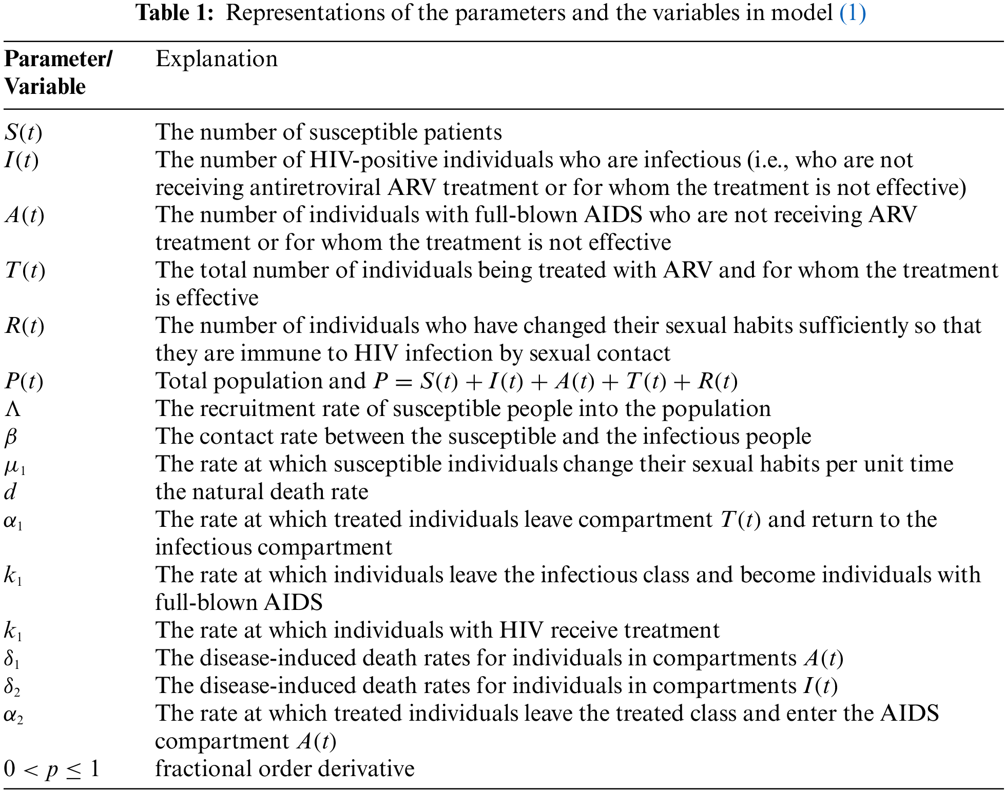
In this study, a numerical method based on the Pell-Lucas polynomials (PLPs) is developed to solve the fractional order HIV/AIDS epidemic model with a treatment compartment. The HIV/AIDS mathematical model with a treatment compartment is divided into five classes, namely, susceptible patients (S), HIV-positive individuals (I), individuals with full-blown AIDS but not receiving ARV treatment (A), individuals being treated (T), and individuals who have changed their sexual habits sufficiently (R). According to the method, by utilizing the PLPs and the collocation points, we convert the fractional order HIV/AIDS epidemic model with a treatment compartment into a nonlinear system of the algebraic equations. Also, the error analysis is presented for the Pell-Lucas approximation method. The aim of this study is to observe the behavior of five populations after days when drug treatment is applied to HIV-infectious and full-blown AIDS people. To demonstrate the usefulness of this method, the applications are made on the numerical example with the help of MATLAB. In addition, four cases of the fractional order derivative () are examined in the range . Owing to applications, we figured out that the outcomes have quite decent errors. Also, we understand that the errors decrease when the value of N increases. The figures in this study are created in MATLAB. The outcomes indicate that the presented method is reasonably sufficient and correct.Keywords
Fractional differential equations are quite popular among scientists in order to model various stable physical phenomena. Recently, fractional order derivatives have attracted great attention due to their numerous applications in nonlinear complex systems arising in fluid mechanics, damping laws, electrical networks, signal processing, diffusion-reaction processes, relaxation processes, electrochemistry, mathematical biology, physics and various important phenomena in other branches of science and engineering. Fractional derivatives provide more precise models of real-life problems than integer order derivatives. Because some systems exhibit memory, history, or non-local effects that may be difficult to model with the help of integer order derivatives, many natural phenomenon problems are modeled utilizing fractional calculus. In recent years, different types of powerful techniques such as the generalized differential transformation method [1], the Adomian decomposition method [2], the homotopy analysis method [3], the homotopy analysis transformation method [4], the modified Laplace transform method [5] and the homotopy perturbation transform method [6,7] have been introduced to find the approximate solution of the fractional model of this type of differential equations.
Fractional differential equations are frequently used in mathematical modeling. Mathematical modeling can provide an understanding of the mechanisms underlying the transmission and spread of disease, help identify key factors in the disease transmission process, recommend effective control and preventive measures, and provide an estimate of the severity and potential scale of the epidemic. Mathematical biology is a multidisciplinary field of study. Mathematical biology is also used as an important tool in medicine, as well as in differential equations, basic sciences, and many fields of engineering such as genetic engineering, biomedical engineering, and clinical engineering. Lately, mathematical biology has been successfully applied to several important fields in medicine including epidemiology, genetics, drug design and discovery, biofluids, cardiovascular diseases, immunology, microbiology, neuroscience, oncology, virology, and more. Thus, medical phenomena are better understood, and practical action paths are found. The improvements in healthcare and quality of life are achieved because there are important contributions such as early diagnosis, effective medicines, and control of epidemics. From past to present, many models such as the logistic equation and the Lotka-Volterra equations based on prey and predator populations [8], HIV (human immunodeficiency virus) infection model [9–12], SIR model (Susceptible-Infected-Removed) and COVID-19 model [13], etc., have been developed in the field of medicine using mathematical biology.
Recently, the studies on mathematical modeling of human immunodeficiency virus (HIV) have become very popular. HIV, which causes the acquired immunodeficiency syndrome (AIDS), devastates the human body’s skill to fight infections. This disease is very hazardous and can be mortal if left untreated. The first AIDS case was detected in 1981 [14]. In 2017, the US Center for Disease Control and Prevention (CDC) [15] declared that if HIV/AIDS is not treated with antiretroviral drugs, HIV infection progresses in several phases. According to some official reports, it is observed that between 2000 and 2016, HIV-related deaths in Africa decreased by one-third thanks to ART (Antiretroviral Therapy) [16]. There are many methods such as the exponential collocation method (ECM) [17], the Bessel collocation method (BCM) [18], the differential transform method (DTM) [19], the optimization method [20], the Galerkin-like method [21], Laplace Adomian decomposition method (LADM) [22], homotopy perturbation method (HPM) [23], variational iteration method (VIM) [24] for solving the HIV infection model. In addition, there are many methods such as homotopy perturbation method, variational iteration method and the Adomian decomposition method (ADM) [25], the fourth kind Chebyshev wavelet method [26], shifted Legendre collocation method [27], the homotopy analysis method [28], LADM [29,30], the Legendre wavelet approach [31], the septic B-spline scheme [32], the fractional approximation method [33] for solving fractional order HIV models. On the other hand, there are some studies conducted for the HIV/AIDS epidemic model with antiretroviral therapy (ART). Luo et al. [34] gave the global stability of disease-free equilibrium and the endemic equilibrium, investigated the long-time stochastic dynamic of the model, and gave some numerical simulations. Wang et al. [35] presented the optimal control problem and conducted numerical simulations. Chen et al. [36] developed a type-2 fuzzy logic controller for antiretroviral therapy of HIV infection and performed simulations for two strategies. Ali et al. [37] constructed the existence and uniqueness conditions of the HIV/AIDS model by utilizing Schaefer and Banachtype fixed point theorems. The model’s qualitative analysis investigated, determined the existence/uniqueness of the solution to the HIV/AIDS model [38], established the stability results for the system by incorporating the Ulam-Hyers method, and applied Newton’s polynomial and the Toufik-Atangana numerical method.
Spectral methods are one of the common methods used for solving mathematical models because they are extremely sensitive. Inasmuch as it uses linear combinations of the orthogonal polynomials as basis functions, these methods lead to accurate approximate solutions [39,40]. Basically, three types of these methods can be identified. These are Tau [41], collocation [42,43] and Galerkin [44] and these are based on orthogonal systems such as Bernstein polynomials, Bessel polynomials, Chebyshev polynomials, Hermite polynomials, Legendre polynomials, Laguerre polynomials, Pell-Lucas polynomials, etc. Compared to other approximation methods, the presented method requires fewer calculations. With the presented method, an approximate solution can be achieved with small N values selected for problems that do not have an exact solution. However, in some methods in the literature, more iterations are required to obtain approximate solutions for systems of the nonlinear equation or even nonlinear equations [45].
On the other hand, there are many methods based on the Pell-Lucas polynomials (PLPs) on the solutions of Fredholm-type delay integro-differential equations [46], functional differential equations [47], population models [8], Fredholm-Volterra integro-differential equations [48], parabolic-type partial integro-differential equations [49], nonlinear Lane-Emden pantograph differential equations [50] and an SIR model on the spread of the novel coronavirus (nCoV-2019) pandemic [13] and very effective results have been obtained from these methods. However, there is no method based on the Pell-Lucas polynomial solutions of the fractional order HIV/AIDS epidemic model with a treatment compartment (FHEMTC) in the literature. This reveals the importance and novelty of this study. For this reason, this study is also important as it is a new application of the method by developing it for fractional problems. In this paper, we consider the following FHEMTC [14,15]:
Representations of parameters and variables in (1) are given in Table 1.
In this study, we examine the approximate solutions based on PLPs of (1):
Here,
Please see [51,52] to learn more about PLPs.
The flow of this paper is created as follows: In Section 2, the required matrix relations of the method are presented. In Section 3, the numerical method for FHEMTC is presented. In Section 4, the error analysis is given. In Section 5, the parameters and initial conditions in the HIV/AIDS epidemic model are determined and Pell-Lucas collocation method (PLCM) is applied to the obtained model. In Section 6, a brief conclusion of the article is presented.
2 Preliminaries and Matrix Relations
In this section, we define the fundamental facts on fractional derivatives and then we express the terms of FHEMTC (1) in matrix form.
Lemma 2.1. PLPs (3) are written the following matrix form [50]:
where,
and
Proof. If the vector
Lemma 2.2. The assumed solution forms (2) can also be written in matrix form as
where,
Proof. If
Definition 2.1. Using [53], we describe the fractional derivative of
for
Here, if
Lemma 2.3. The matrix forms of the p-th order fractional derivatives of the assumed solution forms (2) in (1) become
Here,
and other matrices are given in Lemma 2.2.
Proof. The p-th order fractional derivative of
Lemma 2.4. The nonlinear term in (1) can be expressed the following matrix form:
Here, all matrices are as in Lemma 2.2.
Proof. Through Lemma 2.2, we write
Lemma 2.5. The initial conditions in (1) can be written with matrix relations
Here,
Proof. By substituting
In this part, PLCM is given for the approximate solution of FHEMTC (1) by utilizing collocation points.
Theorem 3.1. Supposed that the approximate solutions of the HIV/AIDS epidemic model (1) are in form (2), then, the following matrix relations are obtained:
Here, all matrices are given in Lemmas 2.2–2.4.
Proof. Firstly, Eq. (7) are written instead of fractional-order derivative terms in model (1), Eq. (9) is written instead of nonlinear term in model (1) and Eq. (5) are written instead of solution forms in the model (1). Hence, the system (11) is obtained, so the proof is completed. ■
Definition 3.1. The collocation points in interval
Theorem 3.2. Assume that the approximate solutions of (1) are given in (5). In that case, FHEMTC (1) becomes as follows:
where,
Also, other matrices are given in Theorem 3.1. and Lemma 2.5.
Proof. The collocation points (12) are substituted into (11) and thus the following system of algebraic equations is obtained:
Now, the relations in (14) are used in the system (15). Then, by writing this system and conditions (10) as a single system, we obtain (13), which completes proof. ■
Corollary 3.1. When nonlinear algebraic system (13) is solved through MATLAB, the unknown coefficients
This section has two purposes. The first purpose is to get an error bound for the presented method. The second purpose is to create an error estimation method. Let
Theorem 4.1. (Upper Boundary of Errors) Assume that the generalized Maclaurin series are represented by
Here,
Proof. Firstly, using the triangle inequality, we can write
Secondly, using Lemma 2.2, we know the matrix representations of the Pell-Lucas polynomial solutions from Lemma 2.2. Therefore, we have
Owing to
Substituting (19) into (18), the following inequalities are obtained:
On the other hand, we can write the remainder terms of the Maclaurin series for
Hence, the following inequalites can be written:
Combining the inequalities (20) and (22) in (17), the inequalities (16) are obtained. So, the proof is completed. ■
Theorem 4.2. (Error Estimation) Assume that the residual functions of FHEMTC (1) for the approximate solutions based on PLPs (2) are represented by
where,
Proof. Inasmuch as the approximate solutions based on PLPs (2) satisfy FHEMTC (1), the proof begins by writing
When system (25) is subtracted from model (1) and the relations in (24) are used, we gain (23). Hence, the proof is completed. ■
Corollary 4.1. If the problem (23) is solved using PLCM in Section 3 for
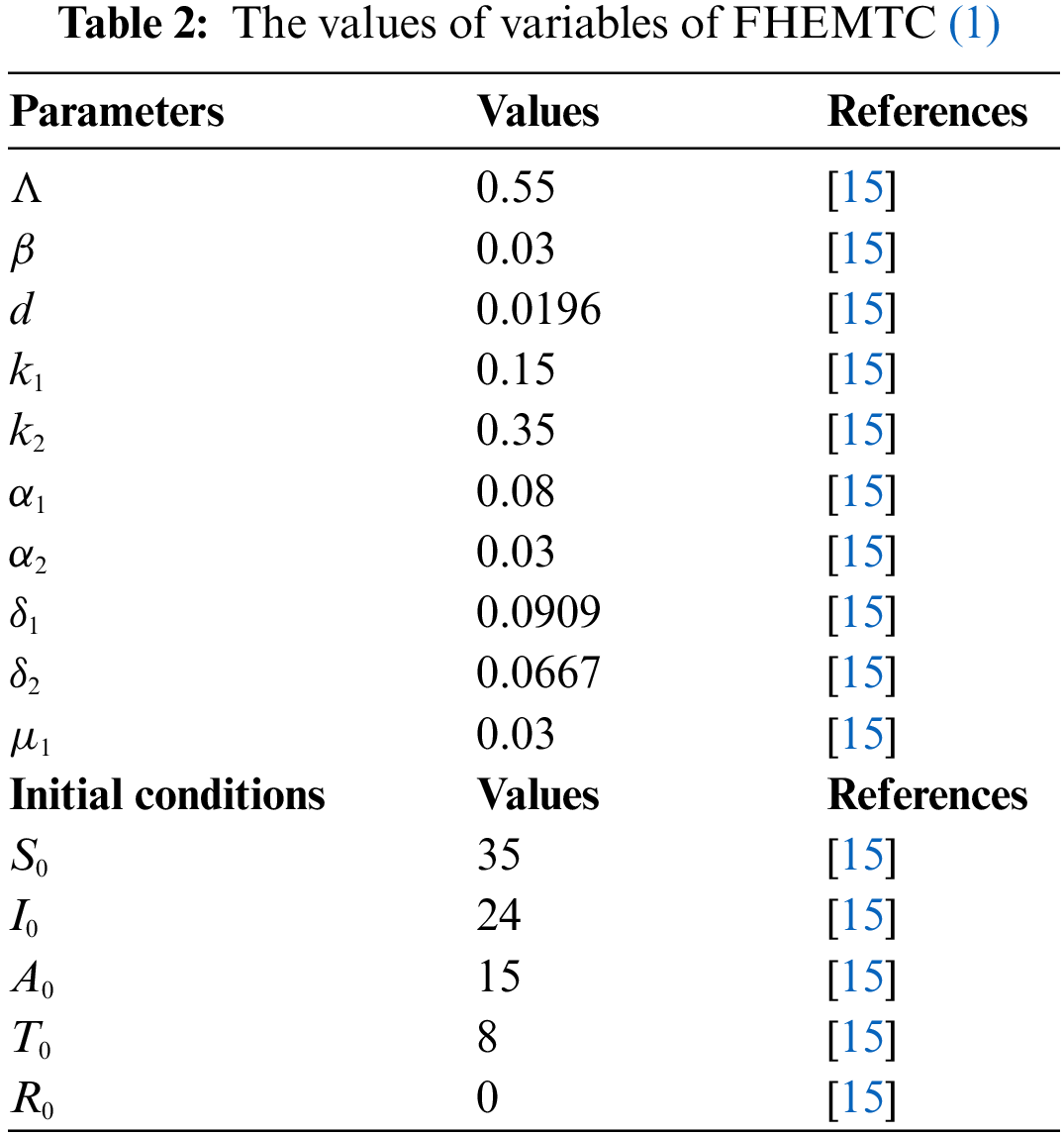
The aim of this section is to show the accuracy and efficiency of the proposed matrix approaches. For this purpose, some numerical computations for FHEMTC (1) are performed. The parameters and initial conditions are determined according to references in [15,37,38] for simulations and these values are given in Table 2. The figures in this study are created in MATLAB.
According to the selected parameters, FHEMTC (1) becomes
When PLCM is applied to the model (26) for
Using Lemma 2.2, the expression (27) is expressed as follows:
Here,
For range
where,
When the relations (10) are used, we have
Here,
Graphical solutions have a lot of importance. For example, thanks to graphical solutions, we can easily understand the behavior of the function, examine the properties of the function, see how it changes for different values of the function, and predict how it changes for different values of the function. Additionally, since we can examine more than one function on the same graph, we can compare the behavior of the functions. In this study, graphical solutions are used since the comparisons are made for different values of the parameter representing the fractional order derivative and for different values of the selected number N.
Fig. 1 shows the graph of functions
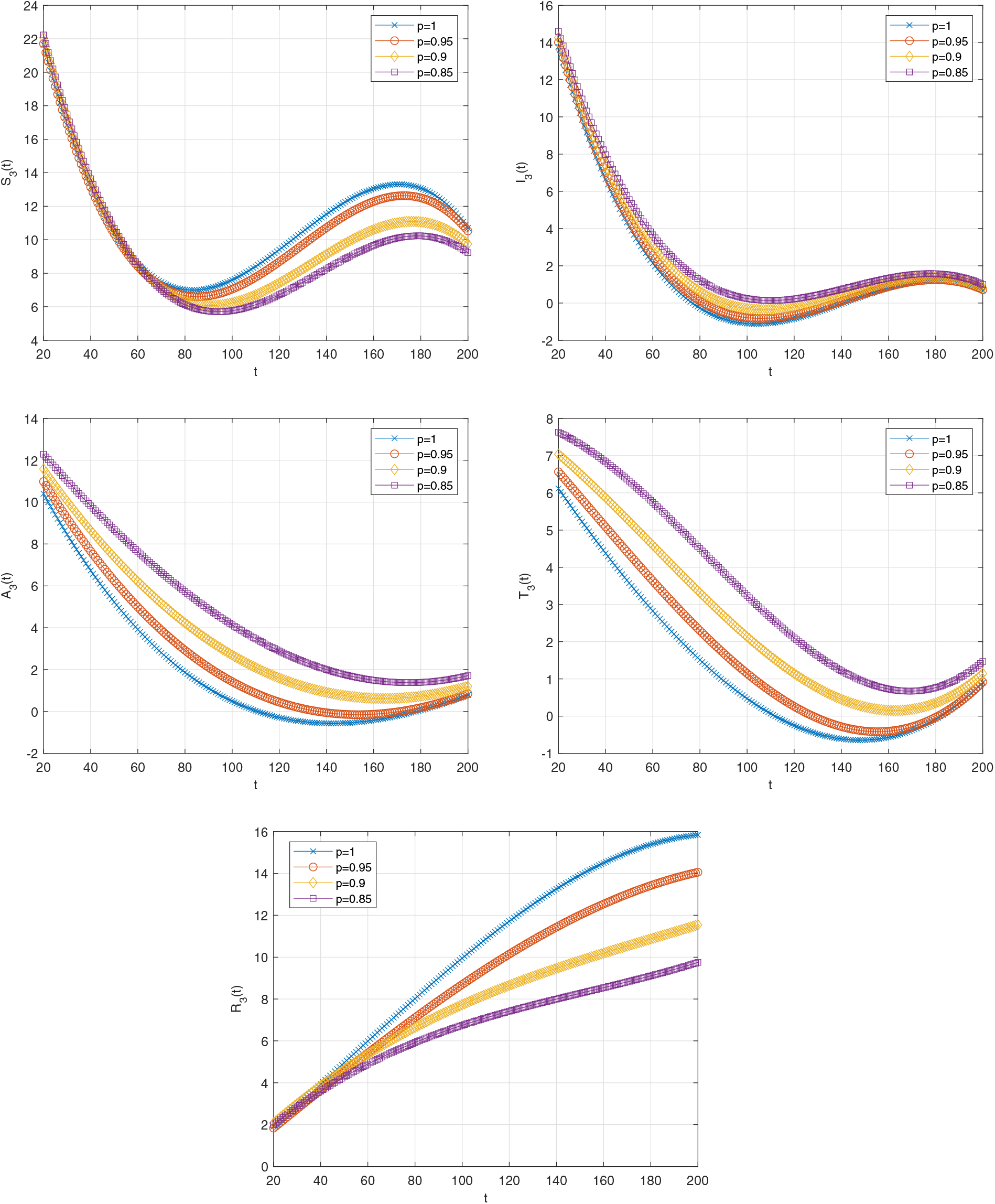
Figure 1: Graph of functions
Fig. 2 demonstrates the graph of solution functions for
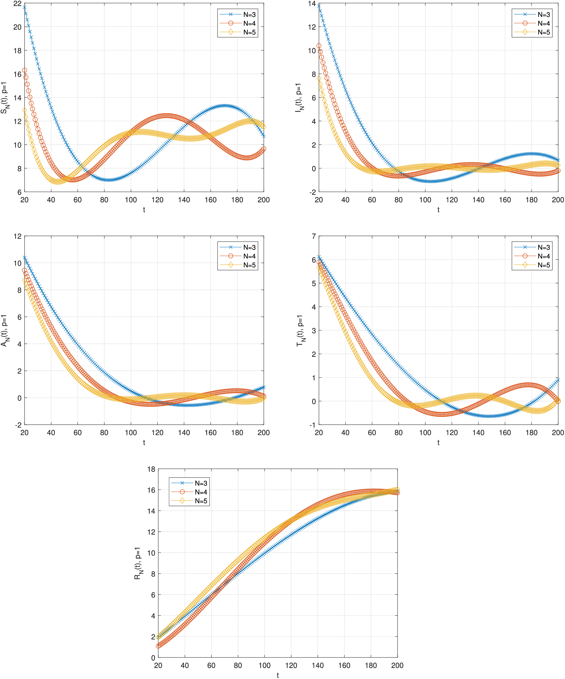
Figure 2: Graph of solution functions of (26) when
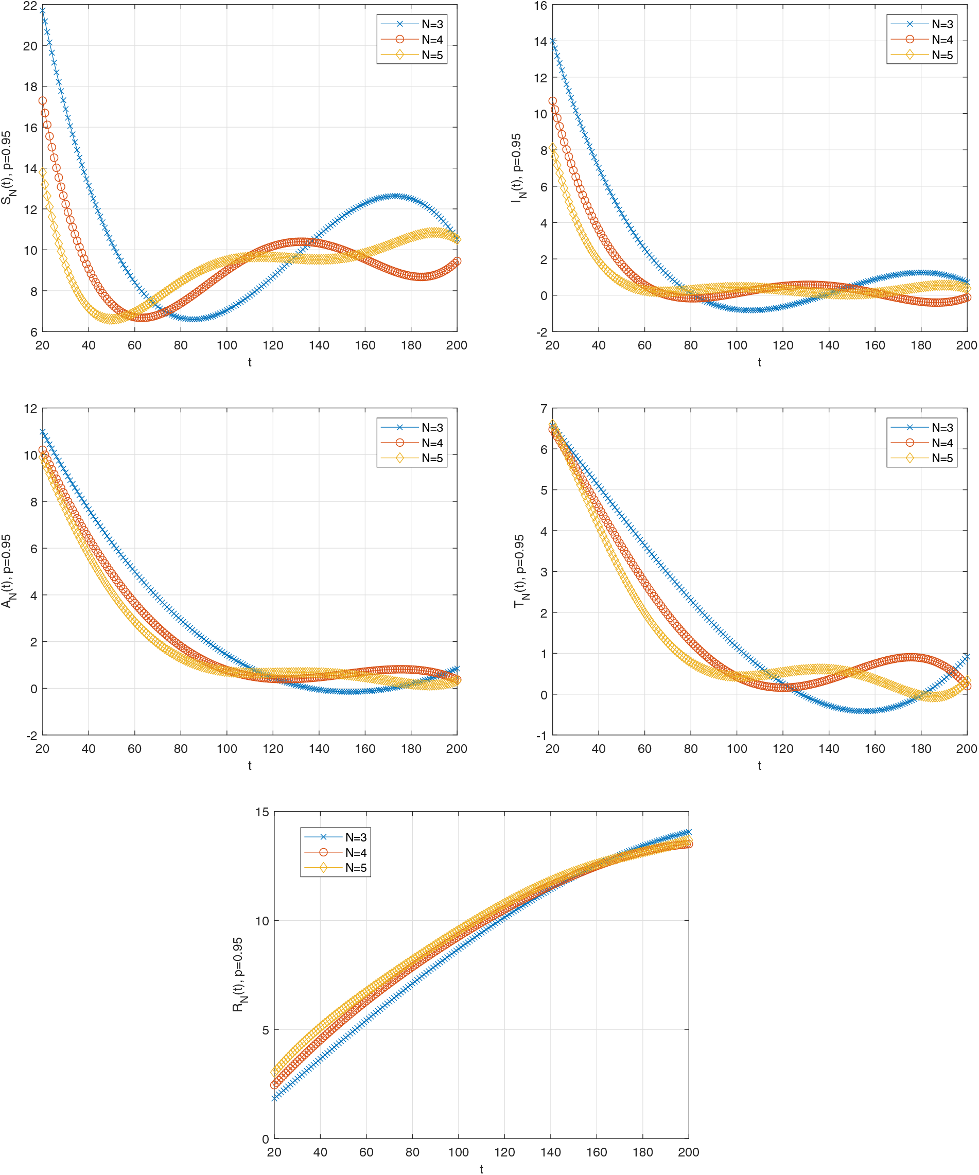
Figure 3: Graph of solution functions of (26) when
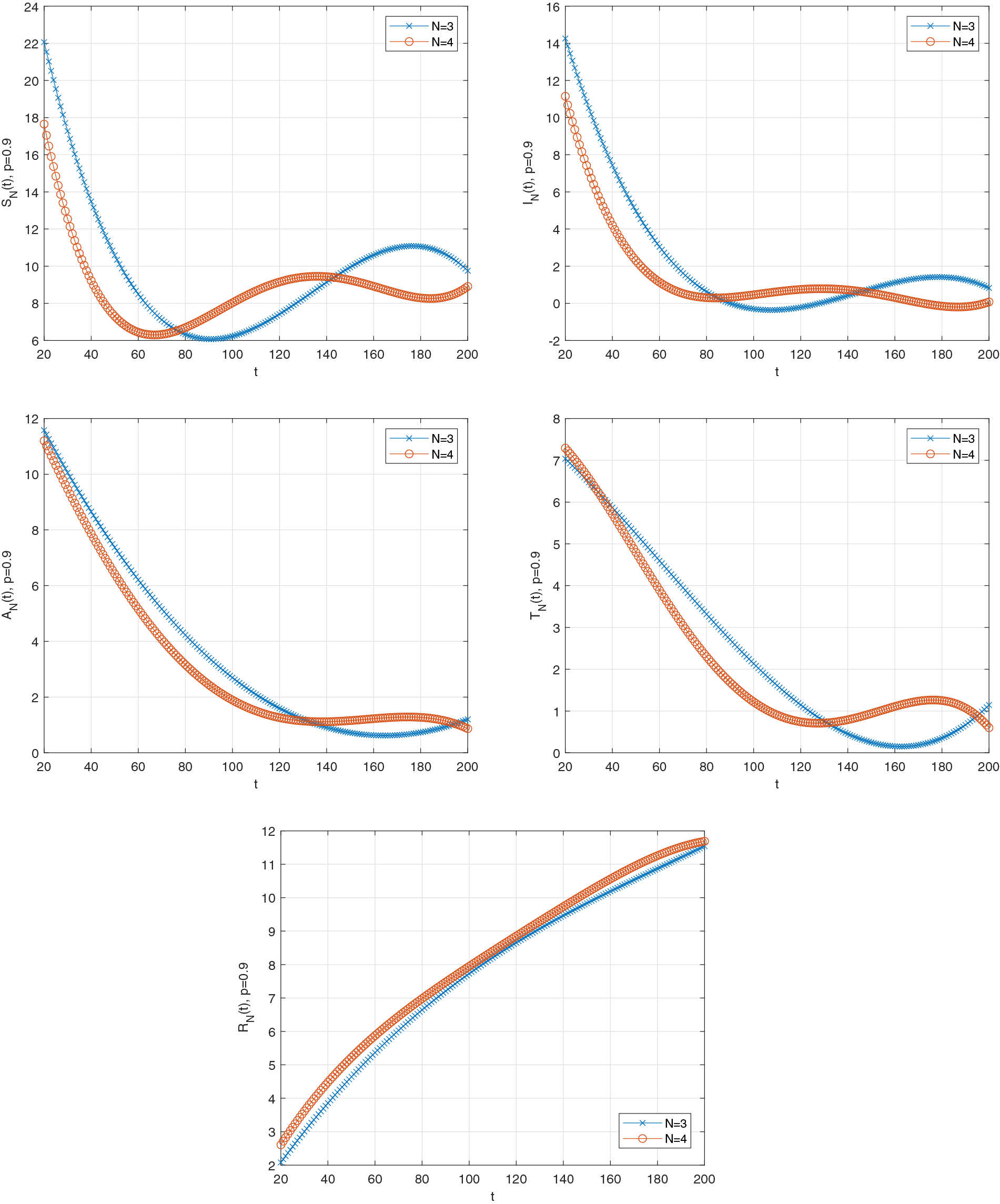
Figure 4: Graph of solution functions of (26) when
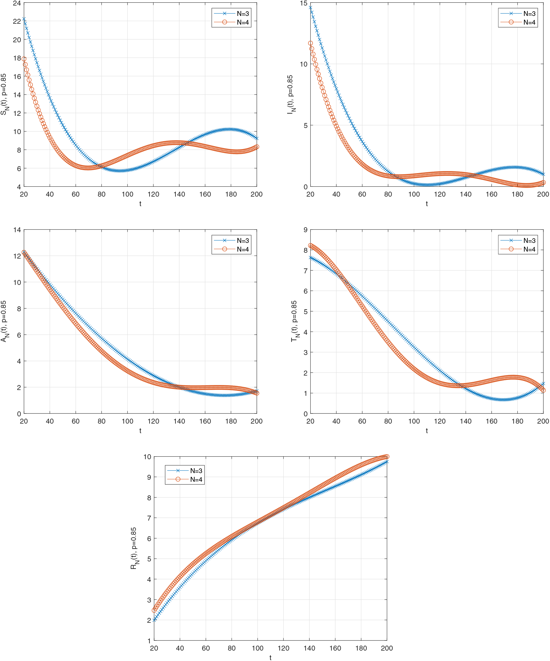
Figure 5: Graph of solution functions of (26) when
Figs. 6–9 show the graph of the estimated error functions, respectively, for various fractional orders (
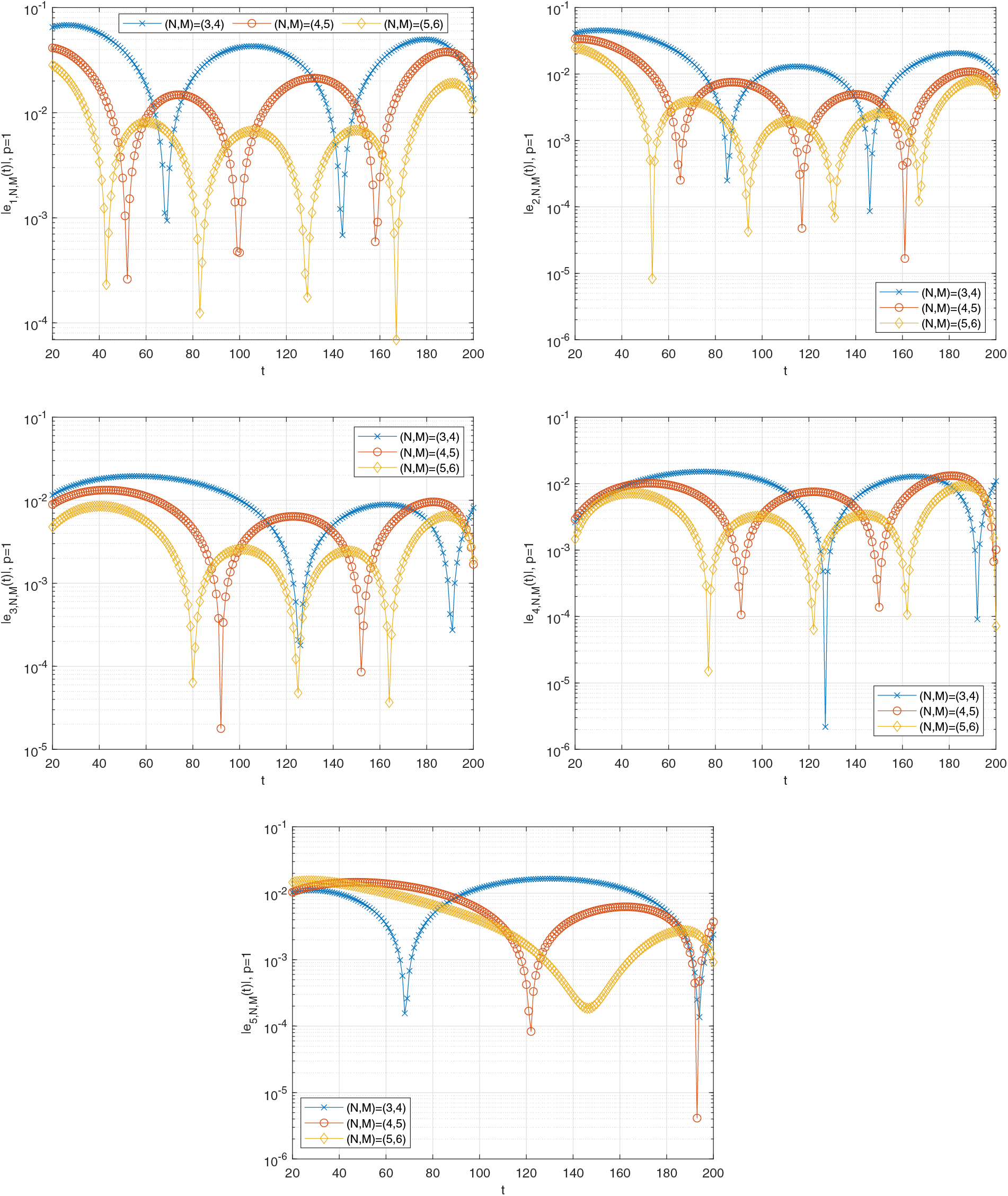
Figure 6: Graph of the estimated errors of (26) when
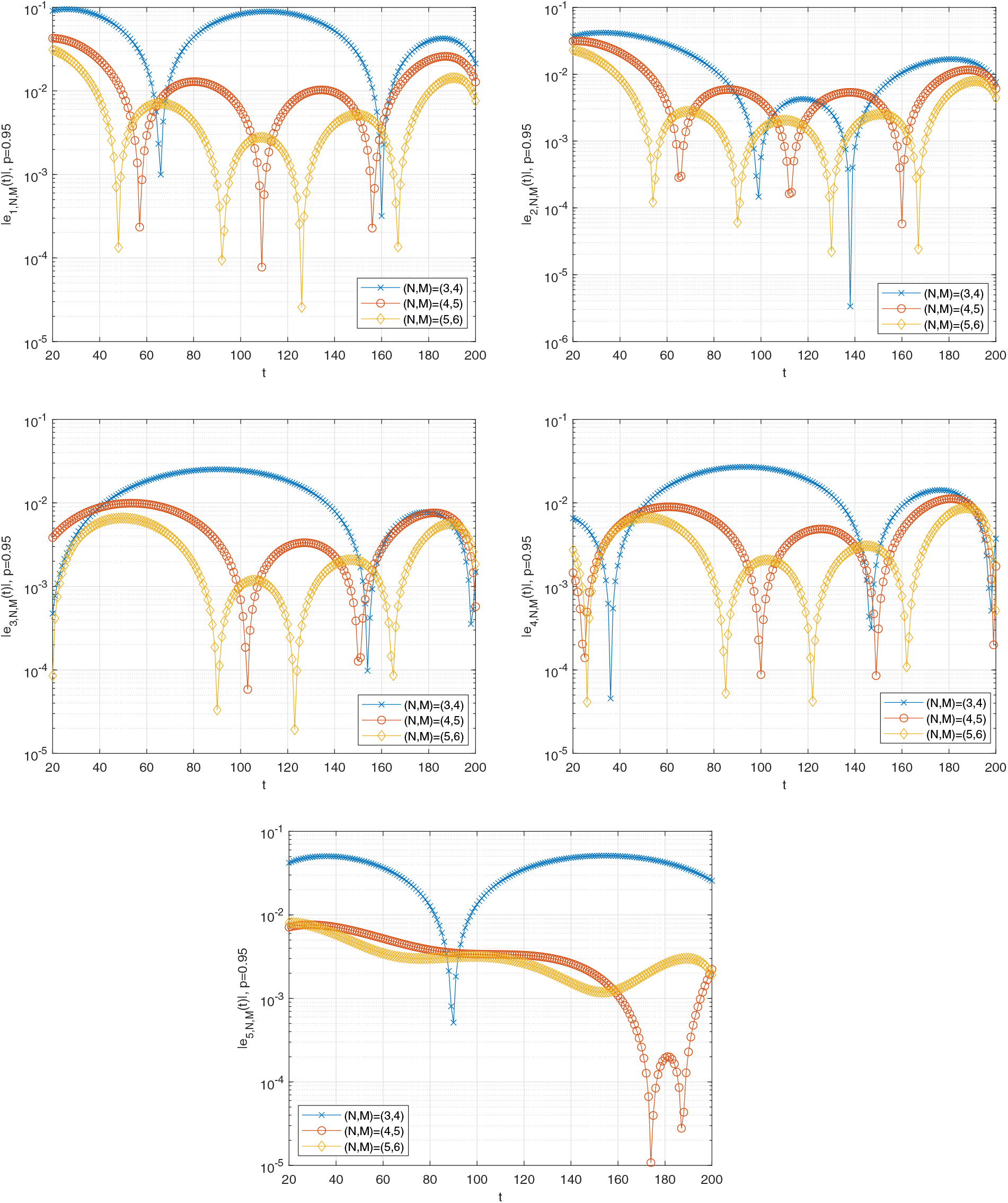
Figure 7: Graph of the estimated errors of (26) when
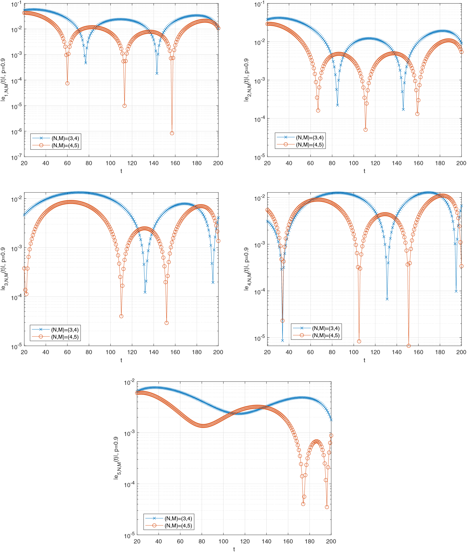
Figure 8: Graph of the estimated errors of (26) when
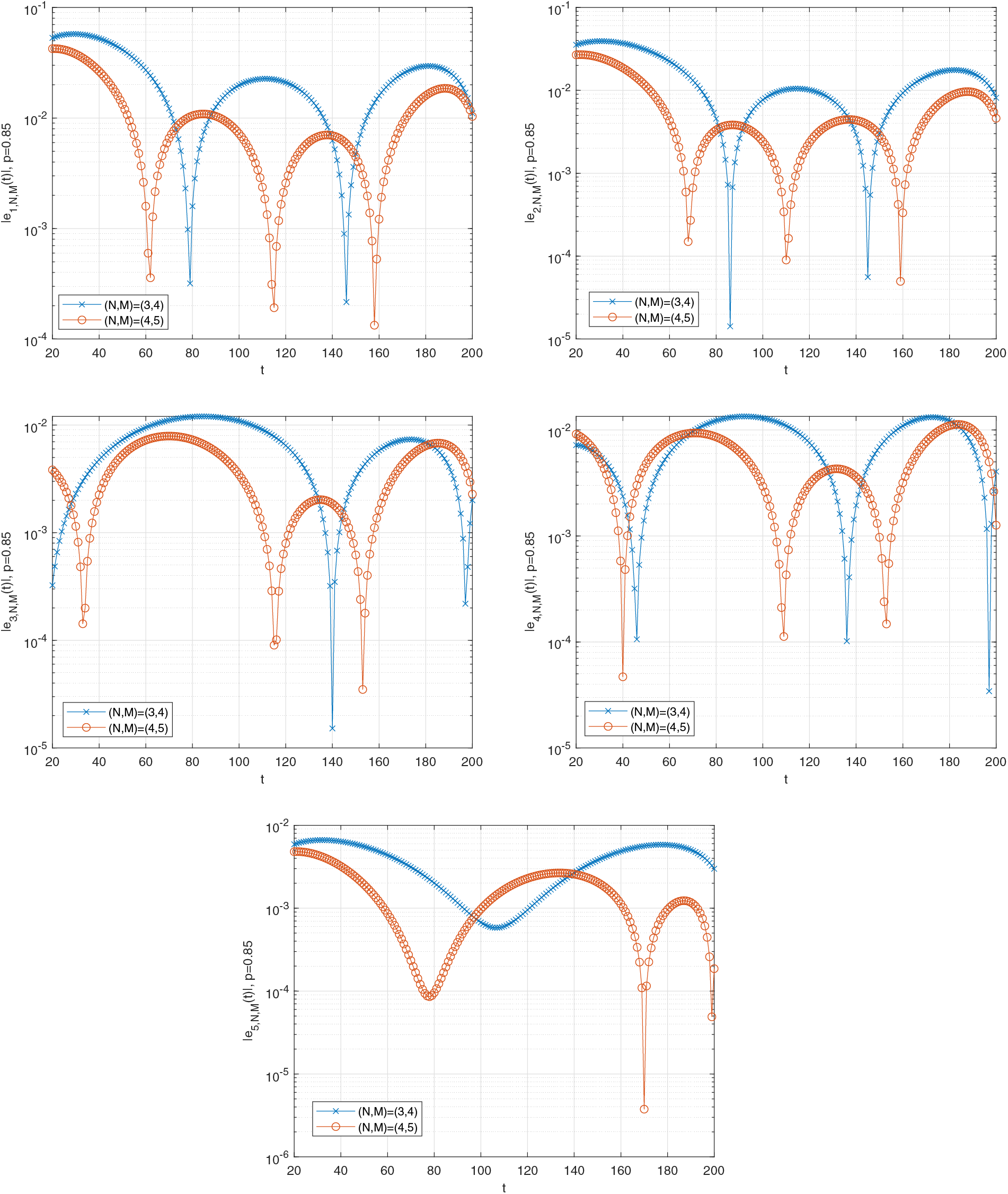
Figure 9: Graph of the estimated errors of (26) when
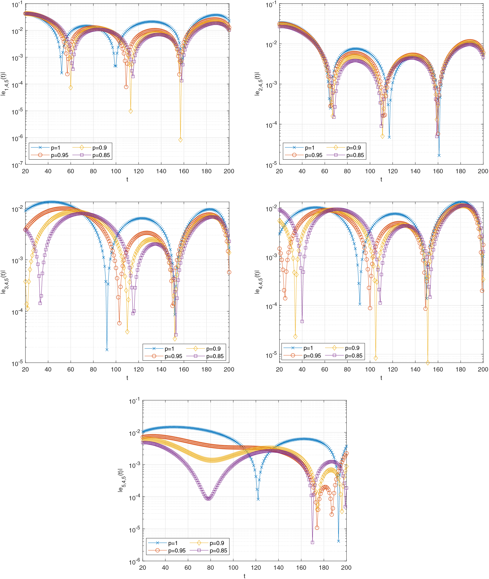
Figure 10: Graph of the estimated errors of (26) when
Moreover, Table 3 gives the values at some
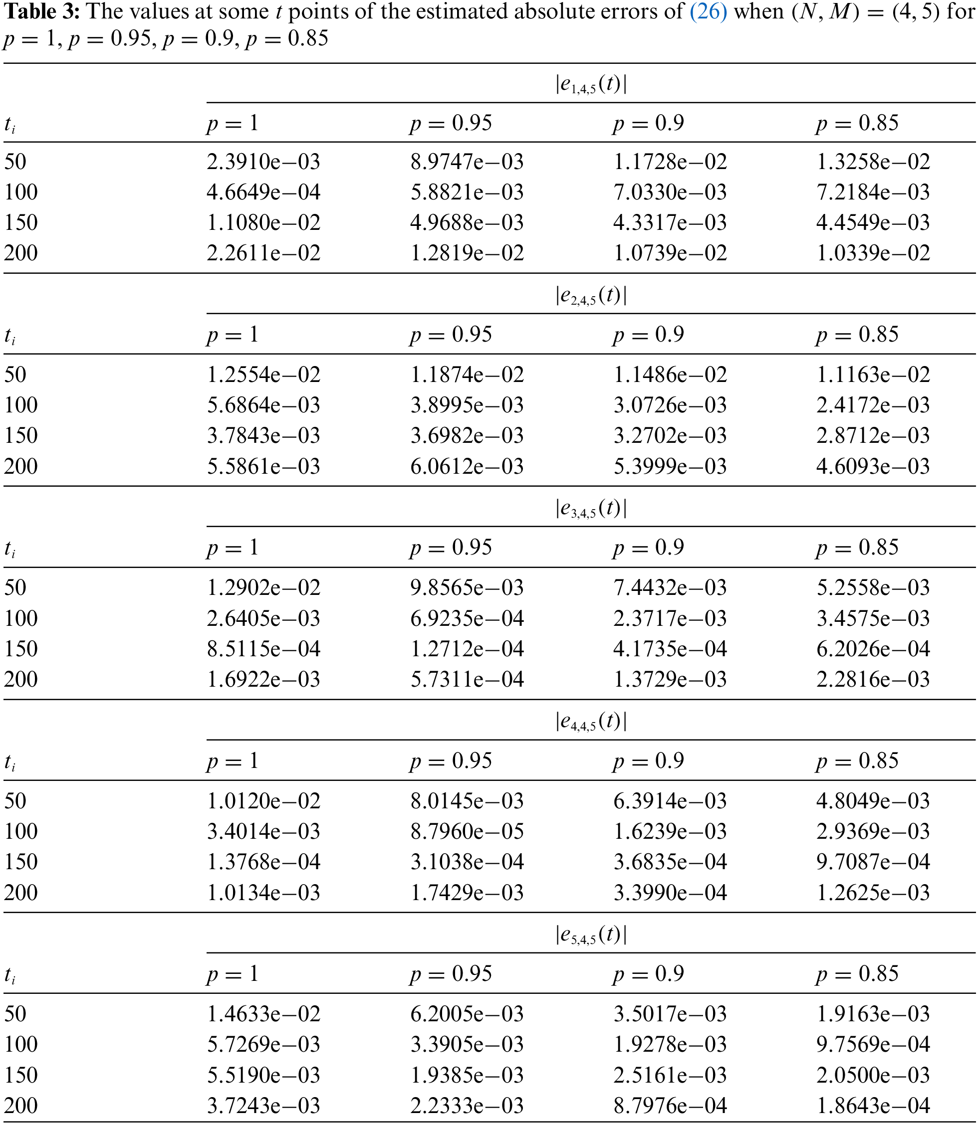
An advantage of the method is that it is prone to computer programming language. Thus, the desired changes can be made to the method easily at any time. For example, the results can be obtained quickly by changing the
In this article, the PLCM is presented to solve FHEMTC. This method is based on Pell-Lucas functions and the collocation method. The fractional derivative is defined in the Caputo type, and the fractional differentiation matrices are derived for PLPs. An error analysis is investigated for the presented method. The error estimation technique is constituted by using residual function. This technique is important because it is possible to comment on the error when an exact solution for the system is not known. In addition, to show the method’s accuracy and efficiency, we analyze four cases of the fractional order derivative within the range
Acknowledgement: The authors would like to thank the reviewers for all helpful comments to improve their manuscript.
Funding Statement: The authors received no specific funding for this study.
Author Contributions: Both authors contributed equally to each section. All authors reviewed the results and approved the final version of the manuscript.
Availability of Data and Materials: All data generated or analyzed during this study are included in this article.
Ethics Approval: Not applicable.
Conflicts of Interest: The authors declare that they have no conflicts of interest to report regarding the present study.
References
1. Liu J, Hou G. Numerical solutions of the space-and time-fractional coupled burgers equations by generalized differential transform method. Appl Math Comput. 2011;217(16):7001–8. doi:10.1016/j.amc.2011.01.111. [Google Scholar] [CrossRef]
2. Momani S, Odibat Z. Analytical solution of a time-fractional Navier–Stokes equation by adomian decomposition method. Appl Math Comput. 2006;177(2):488–94. doi:10.1016/j.amc.2005.11.025. [Google Scholar] [CrossRef]
3. Sakar MG, Erdogan F. The homotopy analysis method for solving the time-fractional Fornberg–Whitham equation and comparison with Adomian’s decomposition method. Appl Math Model. 2013;37(20–21):8876–85. doi:10.1016/j.apm.2013.03.074. [Google Scholar] [CrossRef]
4. Kumar S, Kumar D. Fractional modelling for BBM-burger equation by using new homotopy analysis transform method. J Assoc Arab Univ Basic Appl Sci. 2014;16(1):16–20. doi:10.1016/j.jaubas.2013.10.002. [Google Scholar] [CrossRef]
5. Kumar S, Kumar D, Abbasbandy S, Rashidi M. Analytical solution of fractional navier–stokes equation by using modified laplace decomposition method. Ain Shams Eng J. 2014;5(2):569–74. doi:10.1016/j.asej.2013.11.004. [Google Scholar] [CrossRef]
6. Momani S, Erjaee GH, Alnasr MH. The modified homotopy perturbation method for solving strongly nonlinear oscillators. Comput Math Appl. 2009;58(11–12):2209–20. doi:10.1016/j.camwa.2009.03.082. [Google Scholar] [CrossRef]
7. Sakar MG, Uludag F, Erdogan F. Numerical solution of time-fractional nonlinear PDEs with proportional delays by homotopy perturbation method. Appl Math Model. 2016;40(13–14):6639–49. doi:10.1016/j.apm.2016.02.005. [Google Scholar] [CrossRef]
8. Yuzbasi S, Yildirim G. Pell-Lucas collocation method for numerical solutions of two population models and residual correction. J Taibah Univ Sci. 2020;14(1):1262–78. doi:10.1080/16583655.2020.1816027. [Google Scholar] [CrossRef]
9. Kheiri H, Jafari M. Stability analysis of a fractional order model for the HIV/AIDS epidemic in a patchy environment. journal of computational and applied mathematics. J Comput Appl Math. 2019;346(7181):323–39. doi:10.1016/j.cam.2018.06.055. [Google Scholar] [CrossRef]
10. Liu H, Zhang JF. Dynamics of two time delays differential equation model to HIV latent infection. Phys A: Stat Mech Appl. 2019;514(1):384–95. doi:10.1016/j.physa.2018.09.087. [Google Scholar] [CrossRef]
11. Djordjevic J, Silva CJ, Torres DF. A stochastic sica epidemic model for HIV transmission. Appl Math Lett. 2018;84:168–75. [Google Scholar]
12. Umar M, Sabir Z, Raja MAZ, Aguilar JG, Amin F, Shoaib M. Neuro-swarm intelligent computing paradigm for nonlinear HIV infection model with CD4+ T-cells. Math Comput Simul. 2021;188:241–53. [Google Scholar]
13. Yuzbasi S, Yildirim G. A Pell-Lucas collocation approach for an SIR model on the spread of the novel coronavirus (SARS CoV-2) pandemic: the case of turkey. Mathematics. 2023;11(3):697. [Google Scholar]
14. Huo H-F, Chen R, Wang X-Y. Modelling and stability of HIV/AIDS epidemic model with treatment. Appl Math Model. 2016;40(13–14):6550–9. [Google Scholar]
15. Moore EJ, Sirisubtawee S, Koonprasert S. A caputo-fabrizio fractional differential equation model for HIV/AIDS with treatment compartment. Adv Differ Equ. 2019;2019(1):1–20. [Google Scholar]
16. Pinto CM, Carvalho AR, Tavares JN. Time-varying pharmacodynamics in a simple non-integer HIV infection model. Math Biosci. 2019;307(3):1–12. doi:10.1016/j.mbs.2018.11.001. [Google Scholar] [PubMed] [CrossRef]
17. Yuzbasi S. An exponential collocation method for the solutions of the HIV infection model of CD4+ T cells. Int J Biomath. 2016;9(3):1650036. doi:10.1142/S1793524516500364. [Google Scholar] [CrossRef]
18. Yuzbasi S. A numerical approach to solve the model for HIV infection of CD4+ T cells. Appl Math Model. 2012;36(12):5876–90. doi:10.1016/j.apm.2011.12.021. [Google Scholar] [CrossRef]
19. Srivastava V, Awasthi M, Kumar S. Numerical approximation for HIV infection of CD4+ T cells mathematical model. Ain Shams Eng J. 2014;5(2):625–9. doi:10.1016/j.asej.2013.12.012. [Google Scholar] [CrossRef]
20. Hassani H, Mehrabi S, Naraghirad E, Naghmachi M, Yüzbaşi S. An optimization method based on the generalized polynomials for a model of HIV infection of CD4+ T cells. Iran J Sci Technol, Trans A: Sci. 2020;44(2):407–16. doi:10.1007/s40995-020-00833-3. [Google Scholar] [CrossRef]
21. Yuzbasi S, Karacayir M. A galerkin-type method for solving a delayed model on HIV infection of CD4+ T-cells. Iran J Sci Technol, Trans A: Sci. 2018;42(3):1087–95. doi:10.1007/s40995-018-0529-5. [Google Scholar] [CrossRef]
22. Ongun M. The laplace adomian decomposition method for solving a model for HIV infection of CD4+ T cells. Math Comput Model. 2011;53(5–6):597–603. doi:10.1016/j.mcm.2010.09.009. [Google Scholar] [CrossRef]
23. Merdan M. Homotopy perturbation method for solving a model for HIV infection of CD4+ T cells. Istanbul Commerce Univ J Sci. 2007;6(12):39–52. [Google Scholar]
24. Merdan MA, Gokdogan AY. On the numerical solution of the model for HIV infection of CD4+ T cells. Comput Math Appl. 2011;62(1):118–23. doi:10.1016/j.camwa.2011.04.058. [Google Scholar] [CrossRef]
25. Ullah R, Ellahi R, Sait S, Mohyud-Din S. On the fractional-order model of HIV-1 infection of CD4+ T-cells under the influence of antiviral drug treatment. J Taibah Univ Sci. 2020;14(1):50–9. doi:10.1080/16583655.2019.1700676. [Google Scholar] [CrossRef]
26. Azodi H, Yaghouti M. A new method based on fourth kind Chebyshev wavelets to a fractional-order model of HIV infection of CD4+ T cells. Comput Methods Diff Equ. 2018;6(3):353–71. [Google Scholar]
27. Mirzaee F, Samadyar N. On the numerical method for solving a system of nonlinear fractional ordinary differential equations arising in HIV infection of CD4+ T cells. Iran J Sci Technol, Trans A: Sci. 2019;43(3):1127–38. doi:10.1007/s40995-018-0560-6. [Google Scholar] [CrossRef]
28. Baleanu D, Mohammadi H, Rezapour S. Analysis of the model of HIV-1 infection of CD4 + T-cell with a new approach of fractional derivative. Adv Differ Equ. 2020;2020(1):1–17. doi:10.1186/s13662-020-02544-w. [Google Scholar] [CrossRef]
29. Lichae BH, Biazar J, Ayati Z. The fractional differential model of HIV-1 infection of CD4+ T-cells with description of the effect of antiviral drug treatment. Comput Math Methods Med. 2019;2019(1):4059549. doi:10.1155/2019/4059549. [Google Scholar] [PubMed] [CrossRef]
30. Haq F, Shah K, Rahman GU, Shahzad M. Numerical analysis of fractional order model of HIV-1 infection of CD4+ T-cells. Comput Methods Diff Equ. 2017;5(1):1–11. [Google Scholar]
31. Kumar S, Kumar R, Singh J, Nisar KS, Kumar D. An efficient numerical scheme for fractional model of HIV-1 infection of CD4+ T-cells with the effect of antiviral drug therapy. Alex Eng J. 2020;59(4):2053–64. doi:10.1016/j.aej.2019.12.046. [Google Scholar] [CrossRef]
32. Abdel-Aty AH, Khater MM, Dutta H, Bouslimi J, Omri M. Computational solutions of the HIV-1 infection of CD4+ T-cells fractional mathematical model that causes acquired immunodeficiency syndrome (aids) with the effect of antiviral drug therapy. Chaos, Solitons Fractals. 2020;139(1):110092. [Google Scholar]
33. Jajarmi A, Baleanu D. A new fractional analysis on the interaction of HIV with CD4+ T-cells. Chaos, Solitons Fractals. 2018;113(1):221–9. doi:10.1016/j.chaos.2018.06.009. [Google Scholar] [CrossRef]
34. Luo Y, Huang J, Teng Z, Liu Q. Role of art and prep treatments in a stochastic HIV/AIDS epidemic model. Math Comput Simul. 2024;221(23):337–57. doi:10.1016/j.matcom.2024.03.010. [Google Scholar] [CrossRef]
35. Wang L, Din A, Wu P. Dynamics and optimal control of a spatial diffusion HIV/AIDS model with antiretrovial therapy and pre-exposure prophylaxis treatments. Math Methods Appl Sci. 2022;45(16):10136–61. doi:10.1002/mma.8359. [Google Scholar] [CrossRef]
36. Chen S-B, Rajaee F, Yousefpour A, Alcaraz R, Chu Y-M, Gómez-Aguilar JF, et al. Antiretroviral therapy of HIV infection using a novel optimal type-2 fuzzy control strategy. Alex Eng J. 2021;60(1):1545–55. doi:10.1016/j.aej.2020.11.009. [Google Scholar] [CrossRef]
37. Ali Z, Rabiei F, Shah K, Khodadadi T. Fractal-fractional order dynamical behavior of an HIV/AIDS epidemic mathematical model. Eur Phys J Plus. 2021;136(1):36. doi:10.1140/epjp/s13360-020-00994-5. [Google Scholar] [CrossRef]
38. Ahmad A, Ali R, Ahmad I, Awwad FA, Ismail EA. Global stability of fractional order HIV/AIDS epidemic model under caputo operator and its computational modeling. Fractal Fract. 2023;7(9):643. doi:10.3390/fractalfract7090643. [Google Scholar] [CrossRef]
39. Canuto C, Hussaini MY, Quarteroni A, Zang TA. Spectral methods: fundamentals in single domains. Berlin Heidelberg: Scientific Computation, Springer-Verlag; 2006. [Google Scholar]
40. Mason JC, Handscomb DC. Chebyshev polynomials. Boca Raton, FL, New York: Chapman and Hall/CRC; 2002 Sep. [Google Scholar]
41. Saadatmandi A, Dehghan M. A tau approach for solution of the space fractional diffusion equation. Comput Math Appl. 2011;62(3):1135–42. doi:10.1016/j.camwa.2011.04.014. [Google Scholar] [CrossRef]
42. Sweilam N, Nagy A, El-Sayed AA. On the numerical solution of space fractional order diffusion equation via shifted Chebyshev polynomials of the third kind. J King Saud Univ-Sci. 2016;28(1):41–7. doi:10.1016/j.jksus.2015.05.002. [Google Scholar] [CrossRef]
43. Sweilam N, Nagy A, El-Sayed AA. Solving time-fractional order telegraph equation via sinc–legendre collocation method. Mediterr J Math. 2016;13(6):5119–33. doi:10.1007/s00009-016-0796-3. [Google Scholar] [CrossRef]
44. Abd-Elhameed W. New Galerkin operational matrix of derivatives for solving Lane-Emden singular-type equations. Eur Phys J Plus. 2015;130(3):1–12. doi:10.1140/epjp/i2015-15052-2. [Google Scholar] [CrossRef]
45. İlhan E. Approximate analytical solutions of differential equations using the variational iteration method (Master’s Thesis). Institute of Science and Technology: USA; 2011. [Google Scholar]
46. Dönmez Demir D, Lukonde AP, Kürkçü ÖK, Sezer M. Pell–Lucas series approach for a class of fredholm-type delay integro-differential equations with variable delays. Math Sci. 2021;15(1):55–64. doi:10.1007/s40096-020-00370-5. [Google Scholar] [CrossRef]
47. Sahin M, Sezer M. Pell-Lucas collocation method for solving high-order functional differential equations with hybrid delays. Celal Bayar Univ J Sci. 2018;14:141–9. [Google Scholar]
48. Yuzbasi S, Yildirim G. Pell-Lucas collocation method to solve high-order linear Fredholm-Volterra integro-differential equations and residual correction. Turk J Math. 2020;44(4):1065–91. doi:10.3906/mat-2002-55 [Google Scholar] [CrossRef]
49. Yuzbasi S, Yildirim G. A collocation method to solve the parabolic-type partial integro-differential equations via Pell-Lucas polynomials. Appl Math Comput. 2022;421:126956. [Google Scholar]
50. Yuzbasi S, Yildirim G. Pell-Lucas collocation method to solve second-order nonlinear Lane-Emden type pantograph differential equations. Fundam Contemp Math Sci. 2022;3(1):75–97. doi:10.54974/fcmathsci.1035760. [Google Scholar] [CrossRef]
51. Horadam A, Mahon Bro J. Pell and Pell-Lucas polynomials. Fibonacci Q. 1985;23:7–20. [Google Scholar]
52. Horadam A, Swita B, Filipponi P. Integration and derivative sequences for Pell and Pell-Lucas polynomials. Fibonacci Q. 1994;32:130–5. [Google Scholar]
53. Kilbas AA, Srivastava HM, Trujillo JJ. Theory and applications of fractional differential equations. In: North-Holland mathematics studies. Amsterdam: Elsevier; 2006. vol. 24. [Google Scholar]
54. Podlubny I. Fractional differential equations: an introduction to fractional derivatives, fractional differential equations, to methods of their solution and some of their applications. New York: Elsevier; 1998. vol. 198. [Google Scholar]
Cite This Article
 Copyright © 2024 The Author(s). Published by Tech Science Press.
This work is licensed under a Creative Commons Attribution 4.0 International License , which permits unrestricted use, distribution, and reproduction in any medium, provided the original work is properly cited.
 Downloads
 Citation Tools