Analysis of Extended Fisher-Kolmogorov Equation in 2D Utilizing the Generalized Finite Difference Method with Supplementary Nodes

1  Introduction

The extended Fisher-Kolmogorov (EFK) nonlinear equation has widely physical applications including traveling waves in reaction-diffusion systems [1] and propagation of domain walls in liquid crystals [2]. The two-dimensional (2D) EFK equation with a bounded domain Ω∈R2 with the boundary Γ is considered as follows:

∂u(x,t)∂t+γΔ2u(x,t)−Δu(x,t)+u3(x,t)−u(x,t)=G(x,t),x=(x,y)∈Ω,t≥0.(1)

Two groups of boundary conditions in this problem are implemented as follows:

u(x,t)=g1(x,t),∂u(x,t)∂n=g2(x,t),x∈Γ,,t≥0,(2)

or

u(x,t)=g3(x,t),Δu(x,t)=g4(x,t),x∈Γ,t≥0.(3)

The corresponding initial condition is

u(x,0)=u0(x),x∈Ω,(4)

in which γ denotes a positive constant, Δ signifies Laplace operator, u0,gj(j=1,2,3,4),andG are all known functions. Here, Ω∈R2 represents a geometric bounded domain, and Γ signifies its boundary.

Various numerical approaches have been utilized for simulating the EFK equation, including the finite difference method (FDM) [3–6], the boundary integral equation (BIE) method [7,8], the finite element method (FEM) [9], and the meshless method [10–12]. Compared to traditional mesh-based methods, the meshless method has been regarded as a competitive technique for numerical analysis in science and engineering applications [13–16]. The method discretizes the problem domain using nodes rather than generating an explicit mesh. These nodes can be irregularly distributed, allowing for greater flexibility and adaptability in handling complex geometries and dynamically changing domains [17–21]. Many efforts for designing and developing highly accurate meshless approaches have been implemented [22–26]. Recently, several meshless methods have been proposed and developed. These methods offer the advantage of generating sparse matrices, making them particularly suitable for large-scale numerical simulations [27]. These methods include the generalized finite difference method (GFDM) [28–32], the localized method of fundamental solutions (LMFS) [33–35], and the localized Chebyshev collocation method (LCCM) [36], though they are not limited to these methods.

This work focuses on extended applications of the GFDM. Lizska and Orkisz [37,38] pioneered the development of the GFDM, where they approximated the partial derivatives of functions in governing equations. The implementation of GFDM involves the integration of Taylor series expansions with moving-least squares (MLS) approximations, thus effectively expressing these derivatives. Due to its exceptional accuracy and efficiency, numerous researchers have employed the GFDM in numerical simulations of various physical problems, which involve the thin plate bending problems [39], the fracture mechanics analysis [40], the nonlinear water waves [41], the nonlinear equal-width equation [42], the transient heat conduction analysis [43], and the anomalous diffusion on surfaces [44].

In this study, we utilize the meshless GFDM to investigate the 2D nonlinear EFK problems. The Crank-Nicolson scheme is employed to discretize the temporal derivative in the EFK equation. The GFDM with Newton iterative method is subsequently employed to address these nonlinear boundary value problems resulting from the temporal discretization. In this implementation, an equal number of supplementary nodes as boundary nodes are imposed on the geometric domain boundary. These supplementary nodes serve the purpose of ensuring a well-determined nonlinear system of equations. Unlike the method in [45], which places supplementary nodes outside the boundary, the primary contribution of the approach developed in this work is the direct placement of supplementary nodes on the boundary. This treatment has the advantage of eliminating the need to manually set the distance parameter between the supplementary nodes and the boundary in the original approach, thereby enhancing the stability of the developed method. The distance parameter is influenced by the size of the geometric domain and the density of the collocation nodes. To validate the efficiency of our proposed approach, several numerical examples with various initial-boundary conditions and complicated computational domains are presented.

2  The Discretization Process of the Nonlinear EFK Equation

The detailed description of the discretization process for both the temporal and spatial domains of the nonlinear EFK equation is provided in this section. This involves the application of the Crank-Nicolson scheme to discretize the temporal domain to generate a system of nonlinear boundary value problems, followed by the utilization of the GFDM for solving the system.

2.1 The Crank-Nicolson Scheme

The n+1 time nodes {t1 = 0, t2,⋯,tn=T} are employed to divide the computational time interval [0, T] into n time intervals. Through employing the Crank-Nicolson (CN) scheme, the EFK Eq. (1) is recast as

u(x, ti+1)−u(x, ti)Δt=12[−γΔ2u(x, ti+1)+Δu(x, i+1)−u3(x, ti+1)+u(x, ti+1)+G(x, ti+1)−γΔ2u(x, ti)+Δu(x,ti)−u3(x,ti)+u(x,ti)+G(x,ti)],i=1, 2,…,n−1,(5)

where Δt=ti+1−ti is the time step size. By rearranging terms, Eq. (5) is simplified as

γΔ2u(x, ti+1)−Δu(x, ti+1)+u3(x, ti+1)+(2Δt−1)u(x,ti+1)=Φ(x, ti,ti+1),i=1, 2,…,n−1,(6)

where

Φ(x, ti, ti+1)=−γΔ2u(x, ti)+Δu(x, ti)−u3(x, ti)+(2Δt+1)u(x, ti)+G(x, ti+1)+G(x, ti).(7)

Following the temporal discretization process, the EFK equation is transformed into the subsequent nonlinear stationary problem at each time node ti+1.

γΔ2u(x)−Δu(x)+u3(x)+(2Δt−1)u(x)=Φ(x),(8)

with two groups of boundary conditions

u(x)=g1(x),∂u(x)∂n=g2(x),(9)

or

u(x)=g3(x),Δu(x)=g4(x).(10)

where gj(x)=gj(x, ti+1)(j = 1, 2, 3, 4), u(x)=u(x, ti+1), and Φ(x)=Φ(x, ti, ti+1).

2.2 The GFDM with Supplementary Nodes

Next, the solutions of Eq. (8) with different group of boundary conditions are obtained by employing the GFDM with supplementary nodes. We first distribute some collocation nodes in the geometric domain. As illustrated in Fig. 1, collocation nodes include three different types: supplementary nodes, boundary nodes, and interior nodes. It is crucial to highlight that the quantity of supplementary nodes along the geometric boundary corresponds to that of boundary nodes. The purpose of introducing supplementary nodes will be elaborated as follows. For the previous GFDM presented in [45], original supplementary nodes were placed outside the boundary as shown in Fig. 1. We need to manually set the distance parameter between the supplementary nodes and the boundary. The choice of this distance parameter affects the accuracy of the GFDM. In the present GFDM, the supplementary nodes are directly distributed on the boundary (namely the midpoint between two adjacent boundary collocation nodes). This treatment has the advantage of eliminating the setting of the distance parameter between the supplementary nodes and the boundary in the traditional GFDM, thereby enhancing the stability of the developed method.

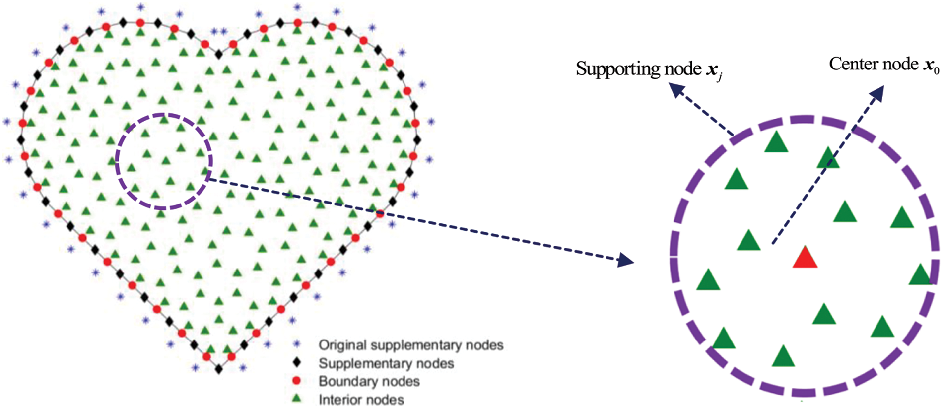
Figure 1: The collocation nodes within the geometric domain, including a local star centered on node x0

Some definitions related with the GFDM are also given to establish the system of equations. A set named as a star is formed for each interior or boundary node x0=(x0, y0) by selecting x0 and its m nearest nodes xj=(xj, yj)(j=1, 2,⋯,m) in all collocation nodes. There is no requirement to establish the star for supplementary nodes. The m nearest nodes centered on node x0 in the local star are referred to as supporting nodes.

For the physical quantities u(xj) at node xj, one can expand them as the following Taylor series at x0 in each star:

u(xj)=∑l=0∞1l!(λj1∂∂x+λj2∂∂y)lu(x0),j=1, 2,…,m.(11)

where λj1=xj−x0,andλj2=yj−y0. Based on the above Taylor series, a residual function ℜ(u) for fourth-order Taylor series expansion is constructed as

ℜ(u)=∑j=1m{[∑l=041l!(λj1∂∂x+λj2∂∂y)lu(x0)−u(xj)]ςj}2,(12)

with the weighting function ςj as

ςj=e−(rj)2−e−(rmax)21−e−(rmax)2,j=1, 2,⋯,m,(13)

where rj=|xj−x0|, and rmax=max1≤j≤m⁡(rj). Some optional weighting functions are available as referenced in [43].

By involving all partial derivatives in Eq. (12), a vector P is formed as

P=[∂u(x0)∂x,∂u(x0)∂y,∂2u(x0)∂x2,∂2u(x0)∂y2,∂2u(x0)∂x∂y…,∂4u(x0)∂x∂y3]T.(14)

Based on ∂ℜ(u)∂{P}=0, a corresponding linear system of equations with coefficients of elements in vector P is derived as

AP=BU,(15)

in which U=[u(x0), u(x1),…,u(xm)]T, A and B are both matrices related with λj1,λj2, and ςj. Interested readers can be referred to [46] for the explicit expressions of matrix A and matrix B. As a result, the partial derivative vector P are derived as linear combinations of u(xj)(j=0, 1,⋯,m) by rewriting Eq. (15) as

P=A−1BU.(16)

After the above implementation, we can obtain the similar form of Eq. (16) for each collocation node.

Substituting the relevant partial derivatives of Eqs. (16) into (8), a system of the nonlinear equation at interior node x0 is derived as

γΔ2u(x0)−Δu(x0)+u3(x0)+(2Δt−1)u(x0)=m0u(x0)+∑j=1mmju(xj)+u3(x0)+(2Δt−1)u(x0),(17)

in which the coefficients mi(i=0, 1,⋯,m) can be determined based on Eq. (16). The above process is also employed for the partial derivatives in boundary conditions (9) or (10) on the geometric boundary, a nonlinear algebraic equation system is finally derived. Here, the coefficient matrix of this nonlinear system is (N1+2N2)×(N1+2N2) dimension (N1 and N2 denote interior node number and boundary node number, respectively). N1+2N2 is also the number of unknown quantities u at all collocation nodes in the nonlinear system. We utilize the “fsolve” solver in MATLAB to solve this system during the implementation. The “fsolve” solver can be regarded as a variant of the Newton-Raphson method. The details of the “fsolve” solver can be found in the URL: https://www.mathworks.com/help/optim/ug/fsolve.html (accessed on 20 January 2024).

Recently, the GFDM based on Taylor series expansions of arbitrary orders was been presented [47], which is slightly more complex to implement numerically. Using higher-order Taylor series expansions can improve the accuracy of the GFDM, but it will also reduce computational efficiency.

3  Numerical Experiments

The proposed method is utilized to simulate three numerical cases in this section. To access the precision of this method, two types of errors are calculated by

Ge=(∑k=1N(u~k−uk)2/∑k=1N(uk)2)1/2,and Me=max1≤k≤N{|u~k−ukuk|},(18)

in which Ge represents the global error, Me signifies the maximum relative error, uk and u~k respectively represent the analytical and numerical results, N signifies the collocation node number. The convergence rate (CA) in space direction is calculated by the formula as

CA=−ln⁡(E2/E1)ln⁡(N2/N1),(19)

in which Ni(i=1, 2) are the number of two different distribution of collocation nodes, and Ei(i=1, 2)=GeorMe represent the corresponding errors of Ni(i=1, 2).

A reference formulation was provided for setting the supporting node number in the local star [47]. Based on this formula, choosing the supporting node number within a relatively large range has minimal impact on the numerical results of the algorithm. Thus, the supporting node number m=50 is applied in a star unless otherwise specified. For all numerical examples, we start by using Hypermesh software to generate the mesh for regions and boundaries. Subsequently, we use only the coordinates of the mesh nodes as collocation nodes for the GFDM.

3.1 Case 1: A Circle Domain

In this case, EFK equation in a circle domain with its center (0, 0) and radius R=0.5 is considered. The boundary conditions are selected as

u(x, y, t)=ex+ysin⁡(at),Δu(x, y, t)=2ex+ysin⁡(at),(20)

and the initial condition is

u(x, y, 0)=0,(21)

in which a>0 is a constant. The function G is

G(x, y, t)=[acos⁡(at)+(4γ−3)sin⁡(at)]ex+y+[sin⁡(at)ex+y]3.(22)

The corresponding analytical solution is derived by boundary conditions and source function. The constants are set to be γ=2 and a=0.1, respectively. The computational time interval is [0,6]s.

In Fig. 2, 139 collocation nodes are distributed throughout the computational domain, with a time step size Δt=0.03s chosen for the simulation process. Fig. 3 exhibits the variation curves for two types of the errors of u. Notably, the maximum relative error Me and global error Ge remain relatively stable with time. Fig. 4 displays the relative errors at final time are obtained by the presented approach with collocation nodes number N=96,112,139 in the circle domain. It is noteworthy that two kinds of errors efficiently decline as collocation nodes number N increasing in Fig. 4.

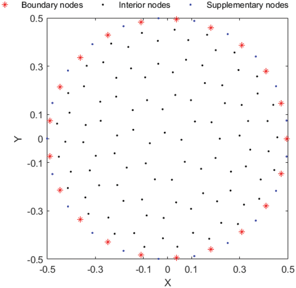
Figure 2: 139 collocation nodes distributed in a circle domain

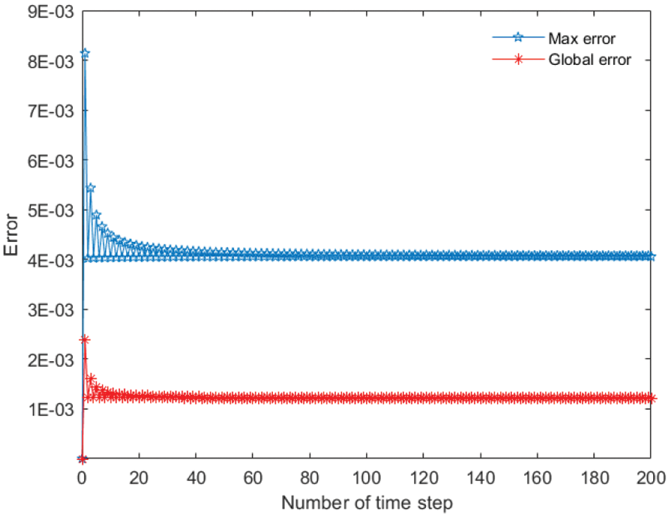
Figure 3: Two types of the errors of u

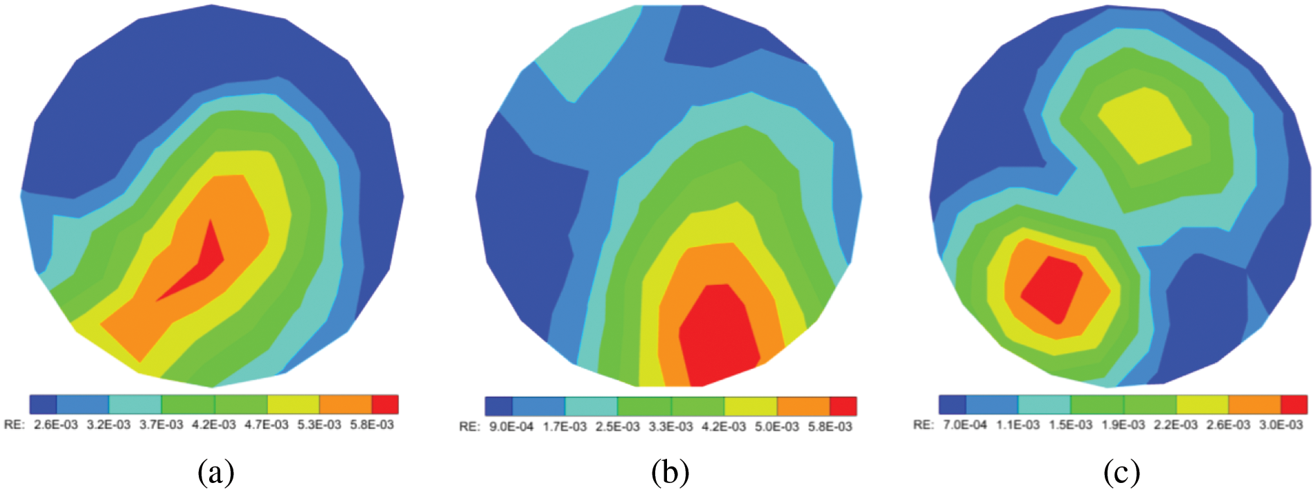
Figure 4: The relative errors of u at collocation nodes number (a) N = 96, (b) N = 112, (c) N = 139

3.2 Case 2: A Gear Model

The EFK equation is simulated in a gear model, and its corresponding dimension is exhibited in Fig. 5a. The boundary conditions are utilized in this case as

u(x, y, t)=e−tcos⁡(x)cos⁡(y)+b,Δu(x,y,t)=−2e−tcos⁡(x)cos⁡(y),(23)

and the initial condition is

u(x, y, 0)=cos⁡(x)cos⁡(y)+b.(24)

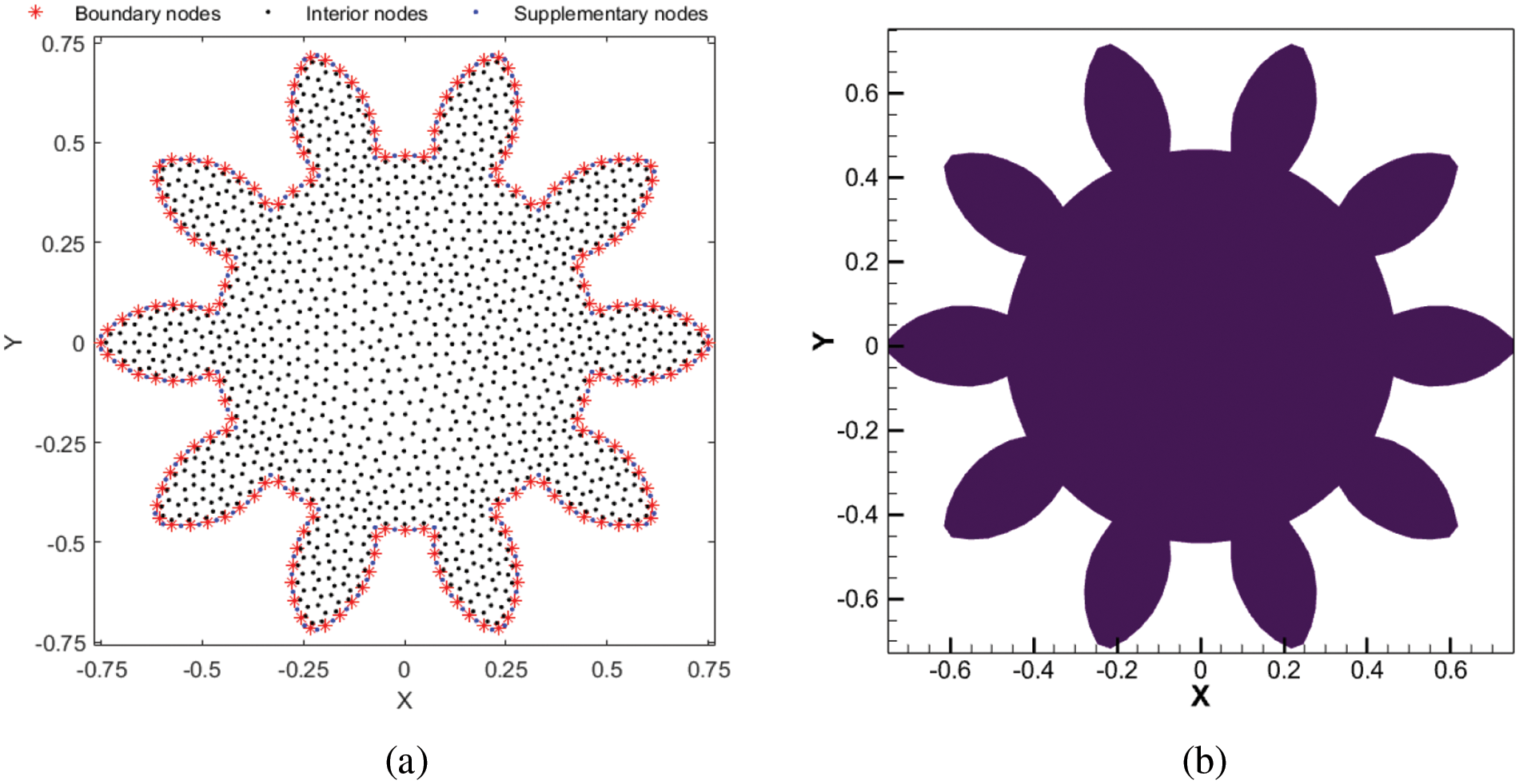
Figure 5: The gear domain (a) and the distribution of 1662 collocation nodes (b)

The source function G is denoted as

G(x, y, t)=4γe−tcos⁡(x)cos⁡(y)+(e−tcos⁡(x)cos⁡(y)+b)3−b(25)

The function u(x, y, t)=e−tcos⁡(x)cos⁡(y)+b is then determined as the analytical solution. The parameters are set to γ=2, b=3. The time span is [0,3] s in the process of numerical simulation.

In Fig. 5b, 1662 collocation nodes are placed within the geometric domain. In this case, the time step size is designated as Δt=0.02s. Fig. 6 describes two kinds of errors curves of u with time. Significantly, the maximum relative error and global error are respectively less than 8.0E-04 and 2.5E-04, respectively. Fig. 7 provides the relative errors of physical quantity u with time t=1s,2s,3s in the gear domain. It is evident from Fig. 7 that the numerical errors highlight the outstanding performance of this method in simulating the EFK equation.

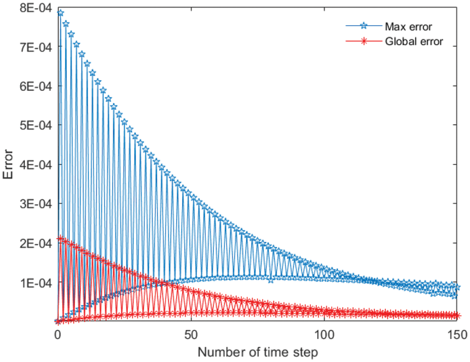
Figure 6: Two types of the errors of u

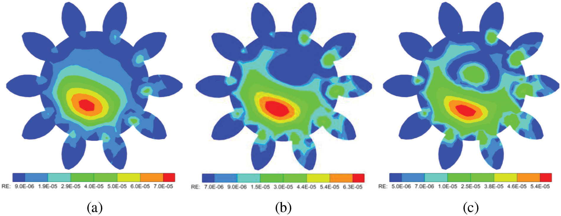
Figure 7: Relative errors of u in the geometric domain for three different time (a) t = 1, (b) t = 2, (c) t = 3

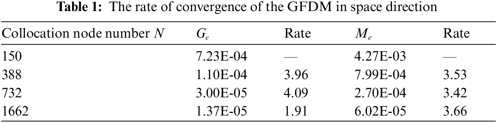
Next, we analyze the spatial convergence rate of the proposed method with the size of time step Δt=0.03, which is determined by utilizing Eq. (19). Table 1 displays the convergence rate of the max relative error (Me) and the global error (Ge) obtained by the present approach. It is demonstrated that the proposed numerical approach exhibits good performance of convergence.

3.3 Case 3: A Sawtooth Domain

The sawtooth model is considered as a computational domain to simulate the EFK equation. The dimension of the sawtooth is shown in Fig. 8a. The boundary conditions are employed in this case as

u(x, y, t)=esin⁡(t)cos⁡(x+y)+c,∂u(x, y, t)∂n=−esin⁡(t)sin⁡(x+y)(n1+n2),(26)

and the initial condition is utilized as

u(x, y, 0)=cos⁡(x+y)+c,(27)

where n=(n1, n2). The source function G is denoted as

G(x, y, t)=(cos⁡(t)+4γ+1)esin⁡(t)cos⁡(x+y)+(esin⁡(t)cos⁡(x+y)+c)3−c(28)

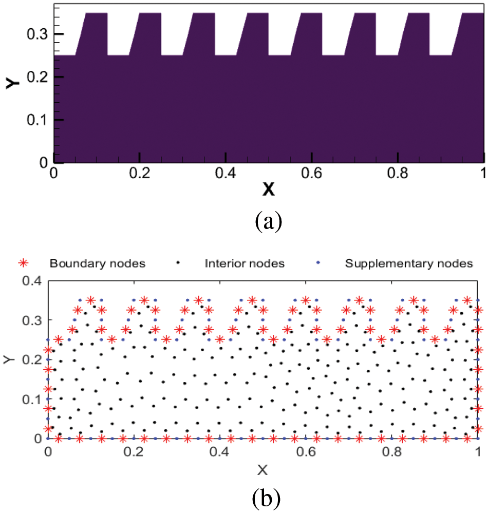
Figure 8: The sawtooth domain (a) and 398 collocation nodes (b)

The positive constants in the EFK equation are γ=2, c=1.

As shown in Fig. 8b, 398 collection nodes distribution are displayed. Fig. 9 plots the relative errors of u in this sawtooth model at time t=15 s with three different time step size Δt=0.75s,0.5s,0.3s. We can distinctly find that, as gradually reducing Δt, the relative errors of u also decrease. This indicates the good convergence of the present approach.

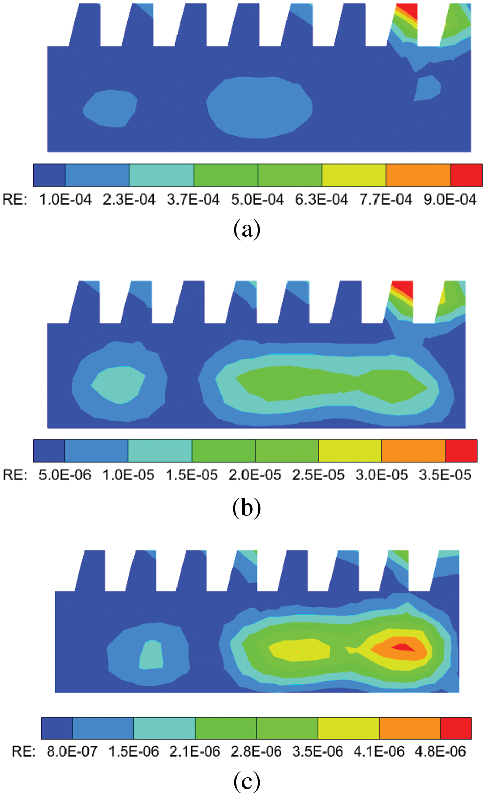
Figure 9: Relative errors of u with (a)Δt=0.75,(b)Δt=0.5,(c)Δt=0.3

4  Conclusions

This study introduces a numerical approach that integrates the GFDM and the Crank-Nicolson scheme for simulating the nonlinear EFK equations under various initial-boundary conditions and complex computational domains. The Crank-Nicolson scheme is employed for discretizing the first-order time derivative in the governing equation. The GFDM that imposes supplementary nodes on the geometric boundary is applied to address the nonlinear boundary value problems after the temporal discretization. The incorporation of supplementary nodes facilitates the efficient establishment of the nonlinear system of equations. The numerical results obtained in three numerical simulations showcase the method’s robust accuracy and convergence when applied to nonlinear EFK equations.

Acknowledgement: The authors would like to take this opportunity to acknowledge the time and effort devoted by reviewers to improving the quality of this work.

Funding Statement: The work described in this paper was supported by the Key Laboratory of Road Construction Technology and Equipment (Chang’an University, No. 300102253502), the Natural Science Foundation of Shandong Province of China (Grant No. ZR2022YQ06), and the Development Plan of Youth Innovation Team in Colleges and Universities of Shandong Province (Grant No. 2022KJ140).

Author Contributions: The authors confirm contribution to the paper as follows: study conception and design: Wenzhen Qu, Yan Gu; data collection: Bingrui Ju, Wenxiang Sun; analysis and interpretation of results: Wenzhen Qu, Yan Gu; draft manuscript preparation: Bingrui Ju, Wenxiang Sun. All authors reviewed the results and approved the final version of the manuscript.

Availability of Data and Materials: All the data used and analyzed is available in the manuscript.

Conflicts of Interest: The authors declare that they have no conflicts of interest to report regarding the present study.

References

1. Ahlers G, Cannell DS. Vortex-front propagation in rotating Couette-Taylor flow. Phys Rev Lett. 1983;50(20):1583. doi:10.1103/PhysRevLett.50.1583. [Google Scholar] [CrossRef]

2. Guozhen Z. Experiments on director waves in nematic liquid crystals. Phys Rev Lett. 1982;49(18):1332. doi:10.1103/PhysRevLett.49.1332. [Google Scholar] [CrossRef]

3. Khiari N, Omrani K. Finite difference discretization of the extended Fisher-Kolmogorov equation in two dimensions. Comput Math Appl. 2011;62(11):4151–60. doi:10.1016/j.camwa.2011.09.065. [Google Scholar] [CrossRef]

4. Kadri T, Omrani K. A fourth-order accurate finite difference scheme for the extended-Fisher-Kolmogorov equation. B Korean Math Soc. 2018;55(1):297–310. doi:10.4134/BKMS.b161013. [Google Scholar] [CrossRef]

5. Li S, Xu D, Zhang J, Sun C. A new three-level fourth-order compact finite difference scheme for the extended Fisher-Kolmogorov equation. Appl Numer Math. 2022;178:41–51. doi:10.1016/j.apnum.2022.03.010. [Google Scholar] [CrossRef]

6. Li S, Kravchenko OV, Qu K. On the L8 convergence of a novel fourth-order compact and conservative difference scheme for the generalized Rosenau-KdV-RLW equation. Numer Algorithms. 2023;94(2):789–816. doi:10.1007/s11075-023-01520-1. [Google Scholar] [CrossRef]

7. Ilati M, Dehghan M. Direct local boundary integral equation method for numerical solution of extended Fisher-Kolmogorov equation. Eng Comput. 2018;34(1):203–13. doi:10.1007/s00366-017-0530-1. [Google Scholar] [CrossRef]

8. Onyejekwe OO. A direct implementation of a modified boundary integral formulation for the extended Fisher-Kolmogorov equation. J Appl Math Phys. 2015;3(10):1262. doi:10.4236/jamp.2015.310155. [Google Scholar] [CrossRef]

9. Doss LJT, Nandini A. An H1-Galerkin mixed finite element method for the extended Fisher-Kolmogorov equation. Int J Numer Anal Model Ser B. 2012;3:460–85. [Google Scholar]

10. Doss LJT, Kousalya N. A finite pointset method for extended Fisher-Kolmogorov equation based on mixed formulation. Int J Comput Methods. 2021;18(1):2050019. doi:10.1142/S021987622050019X. [Google Scholar] [CrossRef]

11. Kumar S, Jiwari R, Mittal R. Radial basis functions based meshfree schemes for the simulation of non-linear extended Fisher-Kolmogorov model. Wave Motion. 2022;109:102863. doi:10.1016/j.wavemoti.2021.102863. [Google Scholar] [CrossRef]

12. Liu F, Cheng Y. The improved element-free Galerkin method based on the nonsingular weight functions for inhomogeneous swelling of polymer gels. Int J Appl Mech. 2018;10(4):1850047. doi:10.1142/S1758825118500473. [Google Scholar] [CrossRef]

13. Chai Y, Li W, Liu Z. Analysis of transient wave propagation dynamics using the enriched finite element method with interpolation cover functions. Appl Math Comput. 2022;412:126564. doi:10.1016/j.amc.2021.126564. [Google Scholar] [CrossRef]

14. Cheng S, Wang F, Wu G, Zhang C. A semi-analytical and boundary-type meshless method with adjoint variable formulation for acoustic design sensitivity analysis. Appl Math Lett. 2022;131:108068. doi:10.1016/j.aml.2022.108068. [Google Scholar] [CrossRef]

15. Wang C, Wang F, Gong Y. Analysis of 2D heat conduction in nonlinear functionally graded materials using a local semi-analytical meshless method. AIMS Math. 2021;6(11):12599–618. doi:10.3934/math.2021726. [Google Scholar] [CrossRef]

16. Li W, Wang F. Precorrected-FFT accelerated singular boundary method for high-frequency acoustic radiation and scattering. Mathematics. 2022;10(2):238. doi:10.3390/math10020238. [Google Scholar] [CrossRef]

17. Li Y, Liu C, Li W, Chai Y. Numerical investigation of the element-free Galerkin method (EFGM) with appropriate temporal discretization techniques for transient wave propagation problems. Appl Math Comput. 2023;442:127755. doi:10.1016/j.amc.2022.127755. [Google Scholar] [CrossRef]

18. Sun T, Wang P, Zhang G, Chai Y. Transient analyses of wave propagations in nonhomogeneous media employing the novel finite element method with the appropriate enrichment function. Comput Math Appl. 2023;129:90–112. doi:10.1016/j.camwa.2022.10.004. [Google Scholar] [CrossRef]

19. Gui Q, Li W, Chai Y. Improved modal analyses using the novel quadrilateral overlapping elements. Comput Math Appl. 2024;154:138–52. doi:10.1016/j.camwa.2023.11.027. [Google Scholar] [CrossRef]

20. Jiang Z, Gui Q, Li W, Chai Y. Assessment of the edge-based smoothed finite element method for dynamic analysis of the multi-phase magneto-electro-elastic structures. Eng Anal Boundary Elem. 2024;163:94–107. doi:10.1016/j.enganabound.2024.02.021. [Google Scholar] [CrossRef]

21. Ju B, Gu Y, Wang R. An enriched radial integration method for evaluating domain integrals in transient boundary element analysis. Appl Math Lett. 2024;153:109067. [Google Scholar]

22. Qiu L, Zhang M, Qin QH. Homogenization function method for time-fractional inverse heat conduction problem in 3D functionally graded materials. Appl Math Lett. 2021;122:107478. [Google Scholar]

23. Li J, Fu Z, Gu Y, Qin QH. Recent advances and emerging applications of the singular boundary method for large-scale and high-frequency computational acoustics. Adv Appl Math Mech. 2021;14:315–343. [Google Scholar]

24. Fu Z, Xi Q, Gu Y, Li J, Qu W, Sun L, et al. Singular boundary method: a review and computer implementation aspects. Eng Anal Boundary Elem. 2023;147:231–66. [Google Scholar]

25. Lin J, Zhang C, Sun L, Lu J. Simulation of seismic wave scattering by embedded cavities in an elastic half-plane using the novel singular boundary method. Adv Appl Math Mech. 2018;10(2):322–42. [Google Scholar]

26. Lin J, Chen W, Wang F. A new investigation into regularization techniques for the method of fundamental solutions. Math Comput Simul. 2011;81(6):1144–52. doi:10.1016/j.matcom.2010.10.030. [Google Scholar] [CrossRef]

27. Fu Z, Tang Z, Xi Q, Liu Q, Gu Y, Wang F. Localized collocation schemes and their applications. Acta Mech Sin. 2022;38(7):422167. doi:10.1007/s10409-022-22167-x. [Google Scholar] [CrossRef]

28. Benito J, Urena F, Gavete L. Influence of several factors in the generalized finite difference method. Appl Math Modell. 2001;25(12):1039–53. doi:10.1016/S0307-904X(01)00029-4. [Google Scholar] [CrossRef]

29. Prieto FU, Muñoz JJB, Corvinos LG. Application of the generalized finite difference method to solve the advection-diffusion equation. J Comput Appl Math. 2011;235(7):1849–55. doi:10.1016/j.cam.2010.05.026. [Google Scholar] [CrossRef]

30. Qu W, Gu Y, Fan CM. A stable numerical framework for long-time dynamic crack analysis. Int J Solids Struct. 2024;293:112768. doi:10.1016/j.ijsolstr.2024.112768. [Google Scholar] [CrossRef]

31. Sun W, Ma H, Qu W. A hybrid numerical method for non-linear transient heat conduction problems with temperature-dependent thermal conductivity. Appl Math Lett. 2024;148:108868. doi:10.1016/j.aml.2023.108868. [Google Scholar] [CrossRef]

32. Fu ZJ, Xie ZY, Ji SY, Tsai CC, Li AL. Meshless generalized finite difference method for water wave interactions with multiple-bottom-seated-cylinder-array structures. Ocean Eng. 2020;195:106736. doi:10.1016/j.oceaneng.2019.106736. [Google Scholar] [CrossRef]

33. Fan C, Huang Y, Chen CS, Kuo S. Localized method of fundamental solutions for solving two-dimensional Laplace and biharmonic equations. Eng Anal Boundary Elem. 2019;101:188–97. doi:10.1016/j.enganabound.2018.11.008. [Google Scholar] [CrossRef]

34. Gu Y, Fan CM, Qu W, Wang F. Localized method of fundamental solutions for large-scale modelling of three-dimensional anisotropic heat conduction problems-theory and MATLAB code. Comput Struct. 2019;220:144–55. doi:10.1016/j.compstruc.2019.04.010. [Google Scholar] [CrossRef]

35. Li W. Localized method of fundamental solutions for 2D harmonic elastic wave problems. Appl Math Lett. 2021;112:106759. doi:10.1016/j.aml.2020.106759. [Google Scholar] [CrossRef]

36. Wang F, Zhao Q, Chen Z, Fan CM. Localized Chebyshev collocation method for solving elliptic partial differential equations in arbitrary 2D domains. Appl Math Comput. 2021;397:125903. doi:10.1016/j.amc.2020.125903. [Google Scholar] [CrossRef]

37. Liszka T. An interpolation method for an irregular net of nodes. Int J Numer Methods Eng. 1984;20(9):1599–612. doi:10.1002/nme.1620200905. [Google Scholar] [CrossRef]

38. Liszka T, Orkisz J. The finite difference method at arbitrary irregular grids and its application in applied mechanics. Comput Struct. 1980;11(1):83–95. doi:10.1016/0045-7949(80)90149-2. [Google Scholar] [CrossRef]

39. Liu F, Song L, Jiang M, Fu G. Generalized finite difference method for solving the bending problem of variable thickness thin plate. Eng Anal Boundary Elem. 2022;139:69–76. doi:10.1016/j.enganabound.2022.03.008. [Google Scholar] [CrossRef]

40. Jiang S, Gu Y, Fan CM, Qu W. Fracture mechanics analysis of bimaterial interface cracks using the generalized finite difference method. Theor Appl Fract Mech. 2021;113:102942. doi:10.1016/j.tafmec.2021.102942. [Google Scholar] [CrossRef]

41. Huang J, Fan CM, Chen JH, Yan J. Meshless generalized finite difference method for the propagation of nonlinear water waves under complex wave conditions. Mathematics. 2022;10(6):1007. doi:10.3390/math10061007. [Google Scholar] [CrossRef]

42. Li PW. The space-time generalized finite difference scheme for solving the nonlinear equal-width equation in the long-time simulation. Appl Math Lett. 2022;132:108181. doi:10.1016/j.aml.2022.108181. [Google Scholar] [CrossRef]

43. Qu W, Gu Y, Zhang Y, Fan CM, Zhang C. A combined scheme of generalized finite difference method and Krylov deferred correction technique for highly accurate solution of transient heat conduction problems. Int J Numer Methods Eng. 2019;117(1):63–83. doi:10.1002/nme.5948. [Google Scholar] [CrossRef]

44. Tang Z, Fu Z, Sun H, Liu X. An efficient localized collocation solver for anomalous diffusion on surfaces. Fract Calc Appl Anal. 2021;24(3):865–94. doi:10.1515/fca-2021-0037. [Google Scholar] [CrossRef]

45. Ju B, Qu W. Three-dimensional application of the meshless generalized finite difference method for solving the extended Fisher-Kolmogorov equation. Appl Math Lett. 2023;136:108458. doi:10.1016/j.aml.2022.108458. [Google Scholar] [CrossRef]

46. Gu Y, Wang L, Chen W, Zhang C, He X. Application of the meshless generalized finite difference method to inverse heat source problems. Int J Heat Mass Transfer. 2017;108:721–29. doi:10.1016/j.ijheatmasstransfer.2016.12.084. [Google Scholar] [CrossRef]

47. Sun W, Qu W, Gu Y, Li PW. An arbitrary order numerical framework for transient heat conduction problems. Int J Heat Mass Transfer. 2024;218:124798. doi:10.1016/j.ijheatmasstransfer.2023.124798. [Google Scholar] [CrossRef]