Optimizing Connections: Applied Shortest Path Algorithms for MANETs

1  Introduction

Information theory has laid the genesis of information technology (IT). From the inception of telephone networks to the recent development of 5th generation (5G) and 6th generation (6G) wireless networks, the rate of development has been unprecedented [1,2]. Following infrastructure, wireless networks are divided into two large categories: infrastructure-based networks and infrastructure-less, or Ad Hoc Networks [3,4]. The idea of Ad Hoc supposes that communicating nodes act without direct, centralized control and communicate directly without dynamical connectivity. Mobile Ad Hoc Networks (MANETs) and the like-Wireless Mesh Networks (WMNs), that is to say, real-world infrastructures-work in exactly this way. One of the points of concern of such networks lies in their decentralized nature and hence poses challenges for security and privacy [5]. MANETs belong to the type Ad Hoc Networks and are part of more mature and stable technologies.

MANET performance is determined by a set of performance factors that include throughput, delay, packet loss, and scalability. Each one of these and others will be routing protocol dependent. The network should be designed such that it is an energy-saver as every device in the network has to work on battery power. These are the new routing techniques for SDN-enabled Wireless Sensor Networks (WSNs) to enhance network efficiency and flexibility. The fuzzy Dijkstra routing will be a version of Dijkstra adapted with fuzzy logic to enhance the routing decisions as defined by AI-Hubaishi et al. [6].

There must be a reasonable analysis and planning of transportation costs, costs of fueling vehicles, and the route network of urban cars shown [7]. They suggested analyzing urban vehicle routes using the Dijkstra's algorithm optimization. Clustering routing algorithms are valuable in MANETs due to their low power consumption and scalable nature. In a clustering system, nodes are organized into clusters, and a leader is appointed to oversee each cluster, as shown in Fig. 1. When the cluster heads have been chosen, the other nodes will form a backbone network that gathers, consolidates, and sends data to the base station along the path that uses the least energy (cost). Using this method increases the network’s longevity significantly.

Figure 1: Clustered network topology in MANETs

Fig. 1 describes two main types of communication in the MANET cluster: single-hop and multi-hop. Direct communication is applicable, in which case, possibly better transmission rates can be acquired since communications will be direct, and hence the latency incurred will be lower than in the case of multi-hop communication. On the other hand, multi-hop communication means that the data passes through at least one intermediary node on its way to the final destination, further delaying the data and extending the scope of the network from the radio range of individual nodes. This is the very fundamental characteristic of MANETs since it can support any kind of flexible network configuration and to conform to node mobility without central infrastructure [8].

Authors in [9,10] devised a new way to choose the cluster head. Node weight in the cluster is calculated using a weighted sum approach, which is subsequently compared to the average weight for that particular cluster. Each connection in a cluster is given a weight function based on a fuzzy membership function and the communication cost between clusters in this approach. Dijkstra’s method uses the whole system with less energy by choosing the path with the least weight.

Liu et al. introduced a multi-hop routing mechanism based on a local competitive and Dijkstra (MRBCD) algorithm in [10]. Cluster Heads (CHs) are elected in MRBCD through a local competitive process, and once elected, they transmit data to the base station employing the path with the lowest overall energy cost. The inter-cluster routing strategy can help to keep inter-cluster connection energy consumption to a minimum. By integrating the two methods, the MRBCD algorithm can balance energy consumption and enhance energy efficiency, thus prolonging the lifespan of wireless sensor networks. One of the most significant and critical challenges in this paper has always been making networks last longer while only using a limited amount of energy. MANETs belong to a category of dynamic networks that are normally not characterized by fixed infrastructure; hence, a very highly dynamic network topology normally ensues. In most cases, efficient routing algorithms, like Dijkstra’s, Bellman-Ford, Open Shortest Path First (OSPF), are considered the backbone to the performance of MANETs, where the shortest path between nodes is determined. While it is the most popular solution for determining the shortest path between nodes, the efficiency of Dijkstra’s algorithm within the dynamic and decentralized nature of MANETs is not always the best. This literature review focuses on shortest-path algorithms proposed for MANETs.

The study of [11] discussed various algorithms and methods used in path planning for robots and Unmanned Aerial Vehicles (UAVs), including A∗ search algorithm, Dijkstra's algorithm, ant algorithms, and particle swarm optimization. It also covers applications in different fields, such as robotics, UAV path planning, and feature subset selection. The paper presents an analysis of three different shortest path-finding algorithms: A∗ Search, Ant Colony Optimization (ACO), and Dijkstra. The paper lacks a comprehensive and in-depth analysis to thoroughly understand how the algorithms perform in finding the shortest path, particularly in the context of MANETs. The study fails to provide realistic solutions or insights due to limitations such as the restricted grid size and the simplistic heuristic calculations employed. Further studies are needed to delve deeper into the performance of these algorithms in MANET environments.

One gap in this paper would be elaborating the number of nodes and its effect on the performance of routing protocols. This is because the scalability of the protocols might be different from each other since it is based on the number of nodes that might take place in the network. Understanding how the protocols behave under a bigger network would be fruitful to make sure the effectiveness of the protocols in practical life, where the number of bode is far more than in a small example. We may also evaluate the effect of the node numbers to obtain the perfect protocol for different network scales, ensuring the efficient and safe run of the communication work in various deployment scenarios. Also, the short path algorithm fails to address finding the short path [12].

The author in [13] did not delve into the scalability of these algorithms for handling large datasets or graphs. Scalability is indispensable for any real-life application, above all in fields like network optimization, artificial intelligence, and big data analytics, which may need to be applied to very large-sized data sets. Without discussing the scalability issue, this could be a big gap since it does apply a limit on any practical application of the paper results in real-world scenarios, where data has volume but is also in motion and complex. This would include studying the way these algorithms scale up with the volume and complexity increase of data, computation complexity, memory usage, and execution time. It would be worth mentioning what optimization techniques are or what alternative algorithms are there that offer better scaling for larger-scale applications. This would make the paper more useful for understanding the practicality and limitations of the algorithms in real life.

It is a weak point of the paper [13], in the sense that it does not go further into analyzing which exact scenarios or conditions Dijkstra’s algorithm will present better performance in comparison to the Bellman-Ford algorithm for many nodes. The paper concludes that for the few nodes in the network, the Bellman-Ford algorithm is efficient, while for many nodes, Dijkstra’s algorithm is efficient and that the causes that would affect this performance need a more comprehensive, all-round analysis. A more detailed examination of graph characteristics is needed. Furthermore, if it has been discussed and turned into real-world applications and situations of common use to those algorithms, it would give practical relevance to this kind of comparison. This paper might also be further improved if the author discussed the limits and assumptions being made during the analysis.

First and foremost, the paper of [14] focuses mainly on comparing A∗ with the Dijkstra algorithm, but it never discusses the dependency of A∗ on heuristic choices or the dynamic environment performance of A∗, its resource consumption and scalability. A much broader review, therefore, is missing, putting into consideration other pathfinding algorithms and, further, practical applications that would underpin the possible limits and strengths of A∗ in practical, real scenarios.

The author in [15] reviewed various studies on hierarchical scale-free networks, small-world properties, and community structure on large networks. It identifies a new class of hierarchical networks with scale-free and fractal features utilized in the structural analyses, such as the average degree, density, clustering coefficient, degree distribution, and average path length. The second complex network aspect of the study on a hierarchical multi-fractal network model is the structural features, including degree distribution, local clustering coefficient, and the average path length. These network properties’ mathematical formulations and proofs are further provided and discussed. Next, the paper cites the known statements on the scaling laws in random and scale-free networks. Finally, some of the aspects in which this model proves what is already known include scaling in random networks, scale-free and fractal structures in hierarchical networks, the small-world effect together with the scale-free property in latter networks with fractal features, as well as the fractal nature and self-similarity in real networks.

The paper of [16] made a critical analysis of the fractal six-star networks used in modeling cellular mobile communication networks with special reference to mean first-passage time (MFPT) and network robustness. The authors introduce an original way of structuring the network that could represent realistic communication systems more correctly. It is mostly involved in the relationship between MFPT and network structure, in which analytical expressions are given to find these times based on the architecture of the network. This part is very crucial since it will help to estimate the efficiency of the signal’s transmission in the whole network, more so in cases of failure in the network. These do reveal that MFPT and the average path length are directly related to the iteration steps of the network and that they relate directly to the size and complexity of the network. A further part of the paper goes into great detail about robustness analysis. In it, the authors define robustness as the ability of the network to carry out work even when some of its nodes are not working. The research will make a study about how it changes with density and concludes high densities generally improve the stability and robustness of the network against failure.

This study proposal, therefore, brings a new way of looking into the performance analysis of Dijkstra’s algorithm in MANETs, indicating that this algorithm outperforms others in sparse graph representations and thus gives tremendous in-depth information well applicable for enhancing routing protocols within dynamic network topologies. The presented paper researches the efficiency and complexity of the Dijkstra's algorithm within the unique context of MANETs. The value of this contribution is in the long-standing literature gap that presented an obstacle to the deepening understanding of algorithmic adaptability and potential optimizations within the environments characterized by fluctuating and decentralized network structures. It would contribute to further development in the underlying theoretical framework and, at the same time, lay the foundation for practical applications in developing more robust and efficient solutions for network designers and researchers working under different dynamic networking scenarios.

This paper aims to increase the complexity of the algorithm that runs behind the routing protocol. Researchers from many fields have come up with many routing methods to make networks use less energy and last longer.

Therefore, this paper aims to apply the Dijkstra’s algorithm to MANETs, focusing on analyzing its complexity and performance, particularly in sparse graph representations, which are characteristic of MANETs.

The structure of the paper is crafted to navigate through a comprehensive analysis of the subject matter. Section 2 probes into the computational complexity inherent to these algorithms, while Section 3 introduces the theoretical underpinnings of computational complexity classes, specifically polynomial (P) and nondeterministic polynomial (NP). Advancing to application, Section 4 highlights innovative routing methodologies utilizing Dijkstra’s algorithm. A critical Comparative Analysis of Dijkstra’s and Bellman-Ford Algorithms is undertaken in Section 5, laying the groundwork for informed contrasts in efficiency and adaptability. The paper reaches its denouement in Section 6, where conclusions are drawn from the synthesized research findings.

2  Computational Complexity

This paper focuses mainly on the use of the Dijkstra's algorithm and Bellman-Ford when used to design the routing protocols in MANETs. Dijkstra’s algorithm is efficient in the sparse network and fast computation without any existing routes, while that of Bellman-Ford has critical robustness against negative weight cycles, which is very important for reliability in unpredictable MANET conditions.

The computational complexities of the algorithms are evaluated and optimized toward the practical effectiveness of MANETs, i.e., high node mobility and resource constraints. This paper, therefore, brings to light the importance of time complexity over space complexity, given that it points out the great need for different kinds of efficiency in handling broad-scale problems within the operational constraints of MANETs.

2.1 Algorithm Complexity-Measure of Magnitude (Worst-Case, Best-Case, and Average-Case Efficiencies)

This quantifies complexity through the algorithm that multiplies the basic steps in computing with the volume of input data. It is designed in a way that the number of such steps generally varies with input data so that the complexity of a typical situation becomes a pertinent measure. The worst-case complexity thus defines the sum of the processes required for obtaining very complex computations. It is more often applied to its approximation of the average case complexity.

Asymptotically tight bounds of complexity functions are expressed in notation. It is also known as the “average case scenario,” which is difficult to determine. The asymptotic tight limit of an algorithm for any random data sequence indicates that the algorithm’s execution time cannot be less than or more than that bound. Fig. 2 presents the upper, lower, and tight limits of the algorithm with running time f(n). Here, n0 is the crossover point. After any value of n>n0, the behavior of the functions will not change. That is, for any value of n greater than n0, f(n) will always grow slower than g(n) (big oh), f(n) always grows faster than g(n) (big omega) or the growth of f(n) will always be wedged between C1⋅g(n) and C2⋅g(n) (big theta). C1 and C2 are constants.

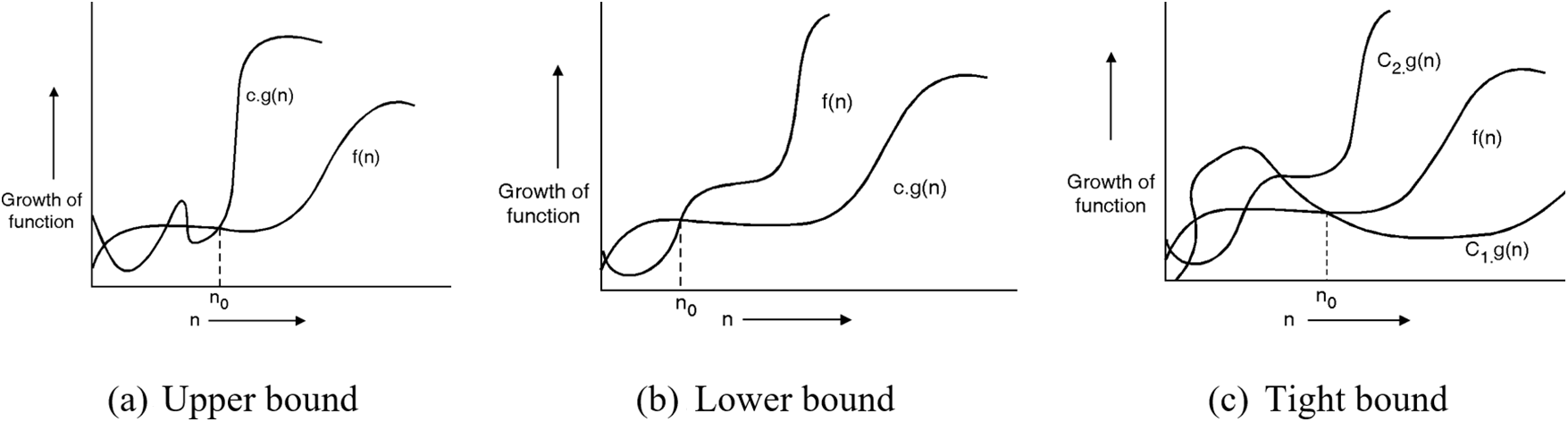
Figure 2: Asymptotic notations representing function growth

The first graph graphically explains the relation of two functions: f(n) and c⋅g(n), with f(n) eventually settling down below c⋅g(n). This illustrates f(n) as being asymptotically upper bounded by c⋅g(n), indicating efficient scaling as n increases.

The second graph displays the behavior of f(n) starting above c⋅g(n) but ultimately leveling off below this threshold, pointing out performance optimization as the problem size increases. This demonstrates the algorithm’s ability to improve its efficiency over time.

The third graph will represent f(n) between these two boundaries— c1⋅g(n) and c2⋅g(n). It outlines f(n) oscillating between the bounds to clarify the oscillations of performance of the algorithm under different operational conditions and parameters.

These graphs further give an insight not only into the scalability and effectiveness of the algorithm but also have particular relevance in MANET environments, where network sizes vary significantly. First, the second overshoot in the second graph indicates how the setup costs are decreasing with the scaling of the systems, which is especially important for large network applications. Thirdly, it bounds the fluctuation graph, which reveals that the algorithm is reliable against a number of network densities and patterns of mobility to give substantial insight into the performance and reliability of deployment scenarios of MANETs.

3  Complexity Classes

Section 2 presents different methods to assess and gauge the efficiency of an algorithm. However, it can also determine and classify the evaluated problem type. For example, issues with the same difficulty level are put together to form complexity classifications. In the literature, there are many different ways to classify how difficult something is, and a few of them are shown here.

3.1 Complexity Class P Problems

The problems of complexity class P, abbreviated as “polynomial,” can be solved by deterministic algorithms in known polynomial time. The algorithm’s time complexity for issues that belong to complexity class P is O(nk), where k is a constant. The value of k depends on the number of frequent operations being performed concerning problem size. For linear search k is 1, for matrix addition k is 2, for matrix multiplication k is 3, etc. Polynomial time cannot be used to address all choice problems. In reality, as opposed to decidable issues, which may be resolved using an algorithm, some are intractable and are undecidable problems. In 1936, Alan Turing gave an example of a problem that could not be solved. It was called the “Halting Problem.”

3.2 Complexity Class NP Problems

NP stands for nondeterministic polynomial. A decision issue of type NP can be addressed using non-deterministic polynomial algorithms. This type of problem is referred to as a nondeterministic polynomial problem. A non-deterministic algorithm is just a two-stage technique in its most basic form. It uses the choice question “I” as an example and then moves on to the next steps. Emphasizing the order in which they improve inefficiency. The O-notation, Ω-notation, and Θ-notation are the most frequently used notations.

4  Time Complexity Analysis of Routing Protocol

In computer networking, the Shortest Path algorithm is used most of the time. It is also used in MANET. Thus, several routing protocols use this technique to discover the shortest route between two points. This method is widely recognized as “Dijkstra’s Shortest Path algorithm.” Employing a starting node and an ending node in a graph, Dijkstra’s algorithm has been applied to find the Shortest Path among the nodes [17]. Once the shortest way to the node having a destination has been reached, the process is claimed to be in its terminating phase. According to Dijkstra, the Energy-Saving Routing Algorithm for Data (ESRAD) is a new routing mechanism for energy-efficient routing in WSN [18]. A way that takes into consideration energy used by electronics in the nodes and then adds that up with that used in the data transmission phase, and selects the way that altogether has the least energy wastage. In that case, it should use the Dijkstra's algorithm to find the path of the least cost from the source node to the destination in the network. It has since become one of the shortest-path problems. For that reason, the Dijkstra algorithm brought a new dawn and became one of the most famous, since it formed the algorithm applied by modern efficient routing protocols. This section further elaborates detailed mechanics of this algorithm and its critical role in routing in dynamic network environments, like MANETs.

4.1 Dijkstra’s Shortest Path Algorithm

Graphs are widely used for expressing distances in data structures. Graphs provide a very great display to mark out the distances from city to city. Dijkstra, in 1959, came up with a graph theory method, which is supposed to find the shortest path. Dijkstra came up with a way that is efficient in seeking the Shortest Path from a given single source on a weighted graph [19–21]. Suppose G is a weighted graph defined by G = (V, E), anyplace V is the set of all vertices, and E is the set of weighted edges. A weighted edge is represented as a cost assigned to each edge. The algorithm’s objective in Shortest Path calculation is to find a path with the minimum cumulative cost incurred to reach point B from point A. Dijkstra’s algorithm presupposes that all weights within the graph are positive, as shown in Fig. 3.

Figure 3: Modifying the distances between nodes in Dijkstra’s algorithm

Below is a breakdown of each individual step involved in Dijkstra’s algorithm:

– Set the distance between the source vertex and all other vertices to zero and set the distance between all other vertices to infinity.

– Make the previous node the source node for the current node and add the other nodes to the list of unvisited vertex list. Calculate the estimated distance between the current node and each of its immediate neighbors’ vertices.

– The value should be updated if the newly computed value is less than the prior value.

– For instance, the present node is denoted by the letter C, and its distance from the source S is equal to the number. Take into account that N is C’s neighbor and that the weight of the edge that connects C and N is 3. Therefore, the distance between source and N, via C, would be 8.

– If the computed distance of N from the source is larger than 8, then update the edge (S, N) to have a distance of 8. Otherwise, do not update it if the estimated distance of N from the source is already greater than 8.

w(S,N)=11w(S,C)+w(C,N)<d(S,N) ⟹ Relax edge(S,N)Update w(S,N)=8 [22,23].(1)

w(S,N)=7w(S,C)+w(C,N)>w(S,N) ⟹ Don't update w(S,N) [22–24].(2)

The described process of finding the shortest path can be encapsulated in the relaxation step, a fundamental operation of Dijkstra's algorithm. For each vertex v adjacent to u, we perform the following operation:

d(v)=min(d(v),d(u)+w(u,v)) [22,23].(3)

In the context of our discussion, let d(v) represent the shortest known distance from the source node to vertex v. Similarly, let w(u,v) denote the weight of the edge between vertices u and v. Furthermore, the min function is utilized to determine the smaller of two given values. In other words, the flowchart in Fig. 4 utilizes the min function to determine that the optimal shorter path will be among the ones obtained by comparing the currently existing distance with the newly calculated one through an adjacent vertex. This method ensures that d(v) reflects the shortest possible route from the source, where d(v) represents the distance from the source to vertex v.

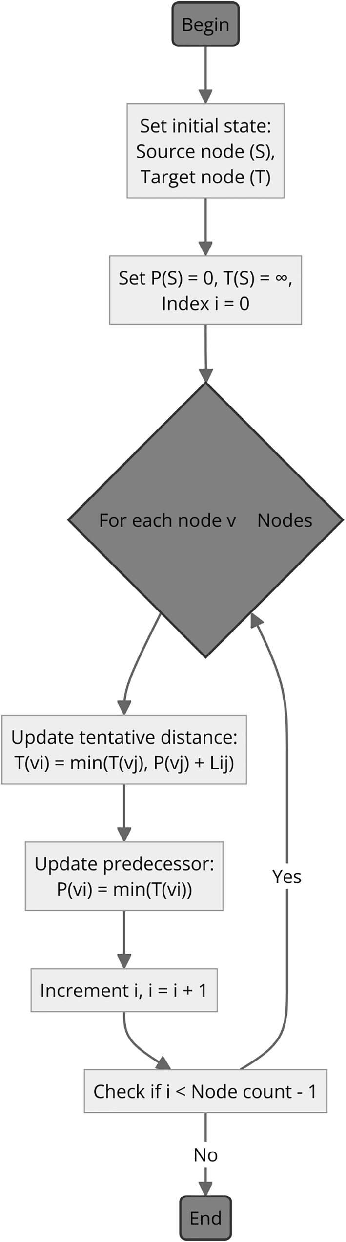
Figure 4: Dijkstra's algorithm flowchart

4.1.1 Applications of Dijkstra’s Shortest Path Algorithm

This section illustrates how Dijkstra’s Shortest Path algorithm is employed in network routing protocols on an effective computation of routes. It profiles an adaptation of the authors in [25], which focuses on the profile of subgraphs to be able to easily and more quickly perform computations in the case of digraphs with nonnegative length. Normalization algorithm combines with Multi-Criteria Decision Making (MCDM), optimizing the route distribution. This will be of great help in logistics and GPS-denied environments, such as subways, to navigate safely but still get the energy efficiencies required [26].

Finally, this section is the Time-Location Penalty Model (TLPM), which tries to overcome the issues on routing precision in road networks due to congestion by adapting Dijkstra’s algorithm in a time-dependent manner but with low memory and resource utilization [27,28].

In order to address the issue of rule requests, Buratti et al. employed Dijkstra’s routing algorithm. The Received Signal Strength Indicator (RSSI) is used to determine the weights of the edges in the network. This term considers an 8-node network topology as shown in Fig. 5. According to the algorithm, each node will be represented by a vertex label with the numbers 1, 2, 3, 4, 5, 6, 7, and 8. As shown in Fig. 5, each edge has a weight associated with it. The network topology shown in Fig. 5 represents a typical setup in a MANET, highlighting the decentralized and dynamic connections between nodes. In MANETs, nodes act as both hosts and routers, forwarding packets to other nodes based on connectivity and proximity. The physical layout depicted here impacts the algorithm’s performance, particularly in how effectively it can find the shortest path without central coordination. Understanding this topology is crucial for deploying MANETs in real-world scenarios like disaster recovery or military operations, where rapid, reliable communication setup is vital.

Figure 5: Directed graph with edge weights

Functioning of the Algorithm as mentioned in the preceding section, the Dijkstra's algorithm operates in a series of iterations. Starting from node 1, kindly refer to Table 1.

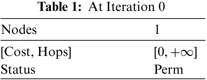
Iteration 0:

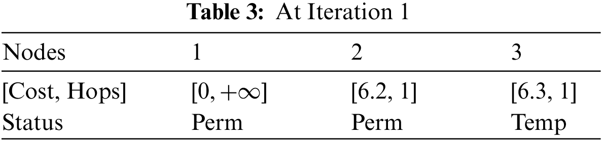
At Iteration 1: Nodes 2 and 3 can be reached directly from node 1, therefore, in Table 2.

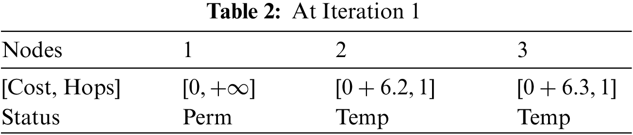
Since the route from node 1 to node 2 is +6.2, smaller than the route from node 1 to node 3, which is +6.3, this information is reflected in Table 3.

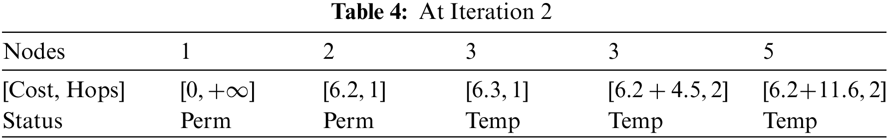
At Iteration 2: Considering node 2 as a new starting node from node 2, could reach node 3 and node 5. The results of Iteration 2 are set out in the Table 4.

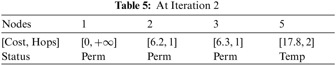
After simplification, kindly refer to Table 5.

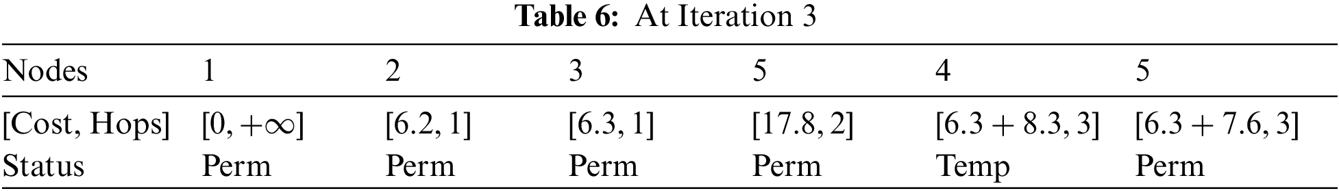
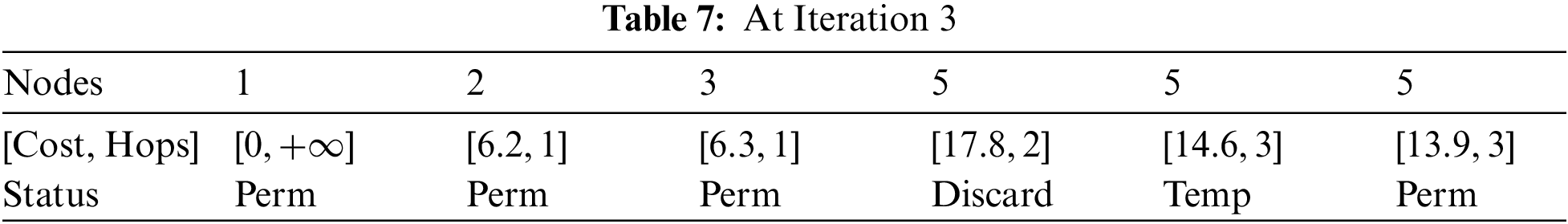
At Iteration 3: Consider node 3. Node 3 is connected to node 4 and node 5 with a cost of 8.3 and 7.6, respectively. Therefore, Table 6 presents updated data.

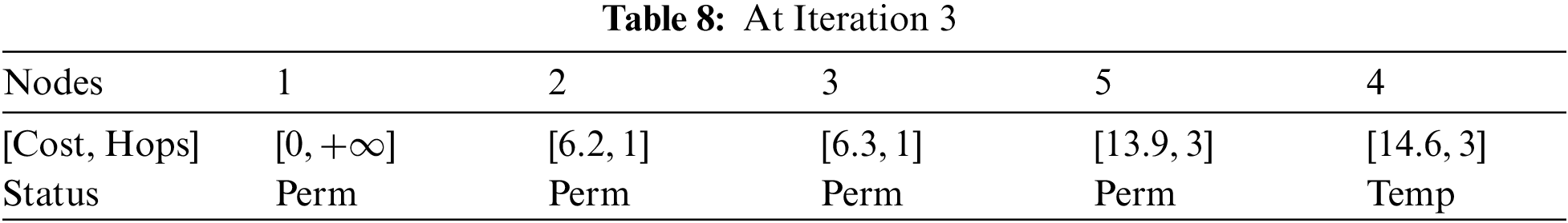
After simplification, refer to Tables 7 and 8.

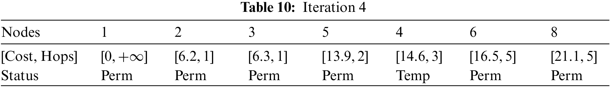
At Iteration 4: Considering node 5, node 6, and node 8 are directly connected, with the cost of 2.6 and 7.2, respectively. Refer to Table 9.

As node 6 is located a short distance from node 5, therefore, it will be marked as permanent as shown in Table 10.

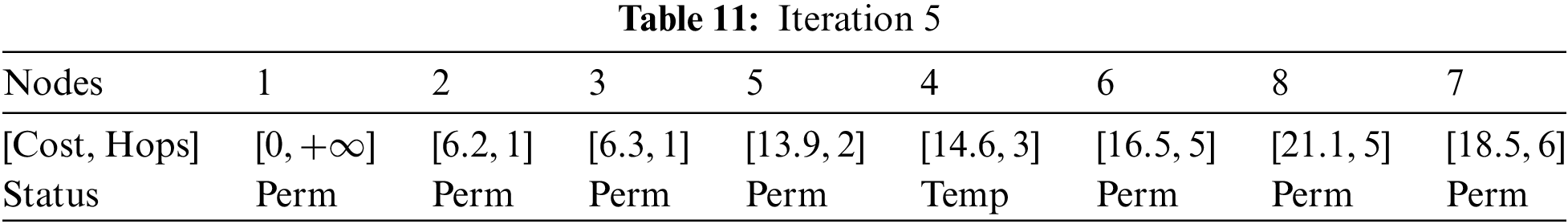
It is now Iteration 5:

Considering node 6, node 7, and node 8 can be reached. After simplification, refer to Table 11.

At Iteration 6: Considering node 7, node 8 can be directly reached. It is shown in Table 12.

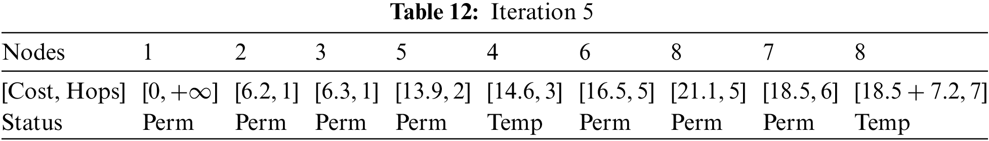
As shown in Table 13, the new path towards node 8 from node 7 has a higher cost.

At Iteration 6: Considering node 7, node 8 can be directly reached.

At Iteration 7: Node 7 can be reached from node 4. The updated data is presented in Table 14.

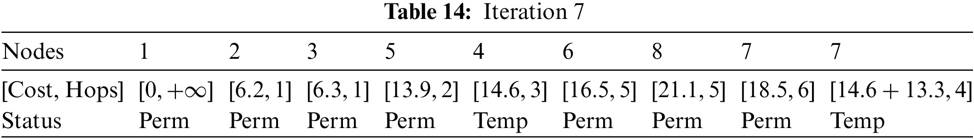
The cost of reaching node 7 is higher, therefore, it will not be considered as shown in Table 15.

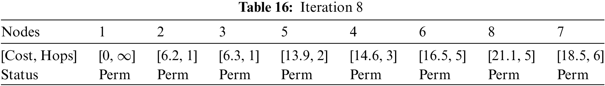
At Iteration 8: Therefore, as node 4 is accessible via node 3 only, the updated data is shown in Table 16.

Thus, the final Dijkstra’s Shortest Path table would be presented in Table 17.

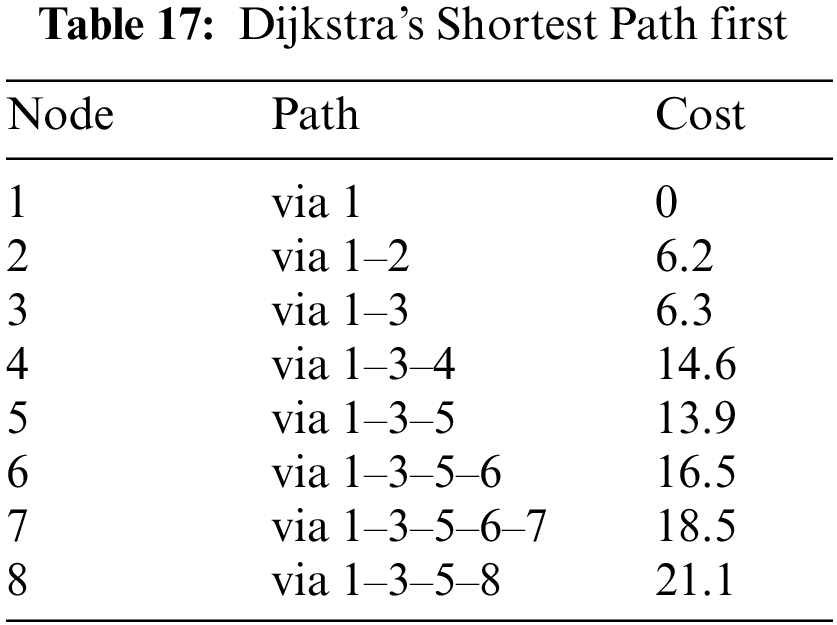
Fig. 6 indicates the comparison between two algorithms concerning the cost efficiency for the determination of the shortest path in a MANET. The cost can be presented in various metrics, including time, energy, or data packets lost. The left one (Dijkstra’s) has low costs attached to it: It is more or less optimized for networks with non-negative weights and finds the shortest paths from the source vertex to all others fairly well. The right-hand side (Bellman-Ford) might have better costs; however, it is very important in dealing with graphs with negative weight cycles, hence offering robust and flexible algorithms in all possible network conditions.

Figure 6: Costs by node with Dijkstra’s algorithm (left) and Bellman-Ford algorithm (right)

4.1.2 Complexity Calculation for Dijkstra’s Algorithm

This section will evaluate the complexity of Dijkstra’s algorithm for finding the Shortest Path. As explained in Section 3, Dijkstra’s algorithm computes the most efficient route between two vertices. Its work is based on weighted edges and directed and undirected graphs. The simplistic implementation approach can use an unsorted array to store the graph’s vertices. Dijkstra’s algorithm searches all the elements in the array (vertices) to find the closest vertices. Since vertices are stored unsorted, the time complexity of initial search will be O(n). This will reduce the total time complexity to O(V2), V corresponds to the number of vertices.

The initial search will have an area complexity of O(V), where V represents the number of vertices. Dijkstra’s algorithm has the worst-case complexity if every node/vertex has to be visited. The steps by which Dijkstra’s algorithm will progress are presented below:

– Begin initializing the vertices array. Each element of the array represents the node of the graph.

– Mark each vertex as unvisited initially.

– The cost or weight must be assigned to each vertex.

– Assign 0 cost to the root vertex and infinity to the rest of the node.

– Set the current node as the root node.

– To find the neighbors of the current node I, calculate the costs by adding the weights of the edges linking the current node and neighbor j to the current node’s cost i>j+i.

– Once all adjacent nodes have been explored, transfer the existing node to the set of visited nodes. Once convergence is reached, there will be no further rechecking.

– The algorithm will stop when all vertices are moved to the visited set.

Dijkstra’s algorithm’s average case time complexity will not be changed; it will remain the same as the worst case because the vertices array is unsorted, and the cost between nodes is unknown initially. Similarly, for the best case, the time complexity of Dijkstra’s algorithm will remain the same due to the above facts. Wang [29] has analyzed the complexity analysis of three different algorithms: Dijkstra’s algorithm, Bellman-Ford algorithm and Floyd-Warshall algorithm. Analysis shows that Dijkstra’s algorithm is suitable for spare graphs, an ideal routing scenario.

However, it has a running time of O(|V|log⁡|V+|E||) in its fastest strongly polynomial implementation employing Fibonacci heaps [30,31]. Although the Bellman-Ford algorithm is ineffective, it is simple to apply in practice. The Floyd-Warshall algorithm is the most inefficient and time-consuming solution to problems involving significant points and edges because it creates unnecessary redundancy in storage space.

4.1.3 Dijkstra’s Algorithm in a Simulated MANET Environment

In this work, the algorithm of Dijkstra works with dynamic and decentralized networks like MANETs to light it up for efficiency and adaptation, live simulation-free. The paper presents a theoretical approach to the application of the algorithm in a hypothesized 8-node MANET model with the key intention of illustrating its ability to accommodate dynamic route changes, which are due to changes in the network conditions. This theoretical analysis emphasizes the potential of Dijkstra for computing routes within the constantly varying network topology, as it is very typical for MANETs, dealing with its computation complexity and operational efficiency. The study reveals insight into the suitableness of the algorithm for the development of routing protocols within decentralized and changing networking environments.

4.2 Bellman-Ford Shortest Path Algorithm

The Bellman-Ford algorithm is categorized as a shortest-path finding algorithm in graph theory, designed to determine the shortest paths from one source vertex to all other vertices in a graph. This is what gives the Bellman-Ford algorithm an upper hand in some applications over the Dijkstra's algorithm, which can only work for graphs that have non-negative numbers assigned to their edges. The Bellman-Ford algorithm works as follows:

•   The process starts with setting the distance from the source vertex to 0, and for all others, it sets the distance to infinity, meaning the shortest path from this point is unknown and assumed to be a path of infinite length.

•   It keeps on updating the distance from the source to the vertex iteratively, always checking whether the use of another vertex v for reaching a certain vertex v could allow reducing the known distance to v. It will then update the distance and predecessor of v to be reconstructed later.

•   This exact process of relaxation for each edge in the graph is done |V|−1 times, where |V | represents the number of vertices in the graph. It therefore guarantees that even in the worst case where the shortest path passes through all the vertices; repetition ensures that the computation of the shortest path is correct.

•   After |V|−1 iterations, an extra iteration checks for negative weight cycles. Where there still exists a possibility that distances can be reduced, that indicates such cycles exist.

The Bellman-Ford algorithm is very useful in networking and routing, where the shortest path or negative cycle detection is concerned. It deals with negative weights; thus, it finds applications in cases where Dijkstra’s algorithm may not apply. Even though it comes with high computation costs, with the time complexity being O(|V||E|), it is still applied in certain scenarios.

4.2.1 Application of Bellman-Ford Algorithm

•   Node 2 is reachable from node 1 with a shortest distance of 6.2.

•   The shortest path to node 3 is from node 1 to node 2 to node 3, with a total distance of 14.5.

•   For node 4, the path is 1→2→3→4, totaling a distance of 19.0.

•   Node 5 is reached via 1→2→3→4→5, with a distance of 22.5.

•   The path to node 8 is 1→2→3→4→5→8, totaling 29.7 in distance.

•   Nodes 6 and 7 are not reachable from node 1, indicating their distances remain at infinity.

Detailed Path Reconstruction

To reconstruct the path for a specific node, like node 8, trace the predecessors back to the source node: 1→2→3→4→5→8.

Thus, the final Shortest Path table would be presented in Table 18.

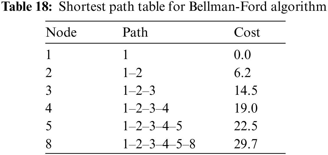
Nodes 6 and 7 are not included as they are not reachable from node 1 with the given topology and edge weights. This indicates that under the current network configuration, there are no paths from node 1 to nodes 6 and 7 that the Bellman-Ford algorithm could identify, reflecting the limitations of connectivity based on the specified graph structure and weights.

5  Comparative Analysis of Dijkstra’s and Bellman-Ford Algorithms

The analysis of Bellman-Ford and Dijkstra’s algorithms in Mobile Ad Hoc Networks (MANETs) highlights their distinct operational characteristics and suitability for different network scenarios.

5.1 Algorithmic Methodology and Performance

The Dijkstra's algorithm is optimal for sparse graphs, often found in MANETs, where it achieves a complexity of O(|V|log⁡(|V|+|E|)) through the use of a Fibonacci heap.

5.2 Assessing Shortest Path Algorithms in MANETs

The paper critically compares the Dijkstra's algorithm and the Bellman-Ford algorithm regarding the MANETs. It is written that Dijkstra’s algorithm was found to be the fastest and most cost-effective of the two. This was especially so in less-dense networks, and hence, in general, the best. Additionally, the supplied Figs. 7 and 8 compare cost efficiency between Dijkstra and Bellman-Ford algorithms on the network nodes as visualized through a bar chart. This conforms with the fact that the Dijkstra's algorithm shows lower costs, while the Bellman-Ford algorithm shows far higher costs. This difference in cost further arises at nodes 5, 6, 8, and so on. Dijkstra still provides the benefit of soft, additive optimization of path costs, while Bellman-Ford, along with its higher costs, is at times needed for networks that need frequent optimization of the paths or that carry out negative cycles to sustain resilience and adaptability.

Figure 7: Cost trajectories for Dijkstra and Bellman-Ford algorithms across nodes

Figure 8: Comparative node costs using Dijkstra and Bellman-Ford algorithms

6  Conclusion

In the world of data transmission, it is vital to zero in on the best pathfinding method. Over the past year, numerous strategies have been devised to address this challenge. Among these, the Dijkstra's algorithm stands out as the preferred method for identifying the minimal route connecting a source to a destination. This document delves into an in-depth analysis of Dijkstra’s algorithm, elucidating its operational steps and evaluating its complexity. It has been noted that the algorithm’s initial time complexity stands at O(n) when vertices are unsorted. Upon completion, the algorithm’s total time complexity reaches O(v2). Nonetheless, employing a Fibonacci heap can significantly enhance efficiency, reducing the time complexity to O(|V|log(|V|+|E|)).

This paper outlines that Dijkstra’s algorithm is the most efficient and computationally gives the best path optimization in MANETs. Analysis carried out proves this to outweigh the Bellman-Ford algorithm, more so on aspects of being cost-effective and practical for routing. Therefore, it is the best alternative because of its efficiency in the shortest path algorithm for sparse graph structures that characterize wireless sensor networks. However, such disadvantages are developed under the basis of simulated MANET environments. The future work involves testing Dijkstra’s algorithm within real MANETs to measure the algorithm performance against real mobile nodes, and different network densities could thus give an overall improvement for routing protocols in dynamic networks.

Acknowledgement: The authors extend their appreciation to the Deanship of Scientific Research at Northern Border University, Arar, Kingdom of Saudi Arabia for funding this research work through the Project Number “NBU-FFR-2024-2248-03”.

Funding Statement: This research was supported by Northern Border University, Arar, Kingdom of Saudi Arabia, through the Project Number “NBU-FFR-2024-2248-03”.

Author Contributions: The specific contributions of each author are as follows: The study conception and design: Ibrahim Alameri, Jitka Komarkova, Tawfik Al-Hadhrami. Data collection: Ibrahim Alameri, Atef Gharbi, Abdulsamad Ebrahim Yahya. Analysis and interpretation of results: Ibrahim Alameri, Jitka Komarkova, Atef Gharbi. Draft manuscript preparation: Ibrahim Alameri, Tawfik Al-Hadhrami, Abdulsamad Ebrahim Yahya, Atef Gharbi, Jitka Komarkova. All authors reviewed the results and approved the final version of the manuscript.

Availability of Data and Materials: The corresponding author can provide data supporting the study’s conclusions upon an adequate request.

Conflicts of Interest: The authors declare that they have no conflicts of interest to report regarding the present study.

References

1. Ge X, Cheng H, Guizani M, Han T. 5G wireless backhaul networks: challenges and research advances. IEEE Netw. 2014;28(6):6–11. doi:10.1109/MNET.2014.6963798. [Google Scholar] [CrossRef]

2. Adil M, Song H, Khan MK, Farouk A, Jin Z. 5G/6G-enabled metaverse technologies: taxonomy, applications, and open security challenges with future research directions. J Netw Comput Appl. 2024;223:103828. doi:10.1016/j.jnca.2024.103828. [Google Scholar] [CrossRef]

3. Alameri I, Komarkova J, Al-Hadhrami T, Lotfi A. Systematic review on modification to the ad-hoc on-demand distance vector routing discovery mechanics. PeerJ Comput Sci. 2022;8(1):e1079. doi:10.7717/peerj-cs.1079. [Google Scholar] [PubMed] [CrossRef]

4. Alameri IA, Komarkova J. Comparative study and analysis of wireless mobile adhoc networks routing protocols. In: Proceedings of the International Masaryk Conference for Ph.D. Students and Young Researchers. Hradec Králové, Czech Republic: Magnanimitas; 2019. Available from: https://dk.upce.cz/handle/10195/75130 [Accessed 2024]. [Google Scholar]

5. Edwin Singh C, Celestin Vigila SM. Fuzzy based intrusion detection system in manet. Meas Sens. 2023;26:100578. doi:10.1016/j.measen.2022.100578. [Google Scholar] [CrossRef]

6. Al-Hubaishi M, Ceken C, Al-Shaikhli A. A novel energy-aware routing mechanism for SDN-enabled wsan. Int J Commun Syst. 2019;32(17):e3724. doi:10.1002/dac.3724. [Google Scholar] [CrossRef]

7. Bing H, Lai L. Improvement and application of Dijkstra algorithms. Acad J Comp Inf Sci. 2022;5(5):97–102. doi:10.25236/AJCIS.2022.050513. [Google Scholar] [CrossRef]

8. Alameri IA, Komarkova J, Al-Hadhrami T. A survey of mobile ad-hoc networks based on fuzzy logic. In: Advances on Intelligent Computing and Data Science, Cham: Springer; 2023. vol. 179, p. 290–9. doi:10.1007/978-3-031-36258-3_25. [Google Scholar] [CrossRef]

9. Razzaq M, Shin S. Fuzzy-logic Dijkstra-based energy-efficient algorithm for data transmission in wsns. Sensors. 2019;19(5):1040. doi:10.3390/s19051040. [Google Scholar] [PubMed] [CrossRef]

10. Liu Q, Liu M. A multi-hop routing mechanism based on local competitive and weighted Dijkstra algorithm for wireless sensor networks. J Phys: Conf Ser. 2020;1621:012074. doi:10.1088/1742-6596/1621/1/012074. [Google Scholar] [CrossRef]

11. Aziz A, Tasfia S, Akhtaruzzaman M. A comparative analysis among three different shortest path-finding algorithms. In: 2022 3rd International Conference for Emerging Technology (INCET); 2022; Belgaum, India. doi:10.1109/INCET54531.2022.9824074. [Google Scholar] [CrossRef]

12. Sampoornam KP, Darshini GR. Performance analysis of bellman Ford, AODV, DSR, ZRP and DYMO routing protocol in manet using exata. In: 2019 International Conference on Advances in Computing and Communication Engineering (ICACCE); 2019; Sathyamangalam, India. doi:10.1109/ICACCE46606.2019.9079958. [Google Scholar] [CrossRef]

13. AbuSalim SW, Ibrahim R, Saringat MZ, Jamel S, Wahab JA. Comparative analysis between Dijkstra and Bellman-Ford algorithms in shortest path optimization. IOP Conf Ser: Mater Sci Eng. 2020;917:012077. doi:10.1088/1757-899X/917/1/012077. [Google Scholar] [CrossRef]

14. Rachmawati D, Gustin L. Analysis of Dijkstra’s algorithm and a* algorithm in shortest path problem. J Phys: Conf Ser. 2020;1566:012061. doi:10.1088/1742-6596/1566/1/012061. [Google Scholar] [CrossRef]

15. Liu JB, Bao Y, Zheng W-T. Analyses of some structural properties on a class of hierarchical scale-free networks. Fractals. 2022;30(7):2250136. doi:10.1142/S0218348X22501365. [Google Scholar] [CrossRef]

16. Liu JB, Zhang X, Cao J, Chen L. Mean first-passage time and robustness of complex cellular mobile communication network. IEEE Trans Netw Sci Eng. 2024;11(3):3066–76. doi:10.1109/TNSE.2024.3358369. [Google Scholar] [CrossRef]

17. Dijkstra EW. A note on two problems in connexion with graphs. In: Edsger Wybe Dijkstra: his life, work, and legacy. 1st edition. New York, NY, USA: Association for Computing Machinery; 2022. p. 287–90. doi:10.1145/3544585.3544600. [Google Scholar] [CrossRef]

18. Yas RM, Hashem SH. A survey on enhancing wire/wireless routing protocol using machine learning algorithms. IOP Conf Ser: Mater Sci Eng. 2020;870:012037. doi:10.1088/1757-899X/870/1/012037. [Google Scholar] [CrossRef]

19. El Gayyar KS, Saleh AI, Labib LM. A new fog-based routing strategy (FBRS) for vehicular ad-hoc networks. Peer Peer Netw Appl. 2022;15(1):1–22. doi:10.1007/s12083-021-01197-0. [Google Scholar] [CrossRef]

20. Shachar A. Introduction to algogens. arXiv preprint arXiv:2403.01426. 2024. [Google Scholar]

21. Mehta DP, Sahni S. Handbook of data structures and applications. New York, USA: Chapman and Hall/CRC; 2004. doi:10.1201/9781420035179 [Accessed 2024]. [Google Scholar] [CrossRef]

22. Cormen TH, Leiserson CE, Rivest RL, Stein C. Introduction to algorithms. USA: MIT Press; 2022. https://dl.ebooksworld.ir/books/Introduction.to.Algorithms.4th.Leiserson.Stein.Rivest.Cormen.MIT.Press.9780262046305.EBooksWorld.ir.pdf. [Google Scholar]

23. Dinitz Y, Itzhak R. Hybrid Bellman–Ford–Dijkstra algorithm. J Discrete Algorithms. 2017;42(4):35–44. doi:10.1016/j.jda.2017.01.001. [Google Scholar] [CrossRef]

24. JinJing Z, Pang L, Kuang X, Jin R. Balancing the qos and security in Dijkstra algorithm by sdn technology. In: Zhang F, Zhai J, Snir M, Jin H, Kasahara H, Valero M, editors. Network and parallel computing. Cham: Springer International Publishing; 2018. vol. 11276, p. 126–131. doi:10.1007/978-3-030-05677-3_11. [Google Scholar] [CrossRef]

25. Akram M, Habib A, Alcantud JCR. An optimization study based on Dijkstra algorithm for a network with trapezoidal picture fuzzy numbers. Neur Comput Appl. 2021;33(4):1329–42. doi:10.1007/s00521-020-05034-y. [Google Scholar] [CrossRef]

26. Rosita YD, Rosyida EE, Rudiyanto MA. Implementation of Dijkstra algorithm and multi-criteria decision-making for optimal route distribution. Procedia Comput Sci. 2019;161(1):378–85. doi:10.1016/j.procs.2019.11.136. [Google Scholar] [CrossRef]

27. Mirzaeinia A, Shahmoradi J, Roghanchi P, Hassanalian M. Autonomous routing and power management of drones in GPS-denied environments through Dijkstra algorithm. In: AIAA Propulsion and Energy 2019 Forum; 2019; Indianapolis IN, USA. doi:10.2514/6.2019-4462. [Google Scholar] [CrossRef]

28. Van den Eynde S, Audenaert JVP, Derudder B, Colle D, Pickavet M. A low-memory alternative for time-dependent Dijkstra. In: 2020 IEEE 23rd International Conference on Intelligent Transportation Systems (ITSC); 2020; Rhodes, Greece. doi:10.1109/ITSC45102.2020.9294640. [Google Scholar] [CrossRef]

29. Wang XZ. The comparison of three algorithms in shortest path issue. J Phys: Conf Ser. 2018;1087:022011. doi:10.1088/1742-6596/1087/2/022011. [Google Scholar] [CrossRef]

30. Fredman ML, Tarjan RE. Fibonacci heaps and their uses in improved network optimization algorithms. J ACM. 1987;34(3):596–615. doi:10.1145/28869.28874. [Google Scholar] [CrossRef]

31. Marcucci T, Umenberger J, Parrilo P, Tedrake R. Shortest paths in graphs of convex sets. SIAM J Optim. 2024;34(1):507–32. doi:10.1137/22M1523790. [Google Scholar] [CrossRef]