Image Hiding with High Robustness Based on Dynamic Region Attention in the Wavelet Domain

1  Introduction

Image encryption typically involves encrypting the entire content of an image, rendering it unreadable and unrecognizable to anyone without the correct decryption key. The purpose of encryption is to ensure the confidentiality of the information, protecting it from being disclosed even if it is intercepted [1,2].

In contrast, image hiding (digital steganography) involves embedding secret information or another image within a host image that appears ordinary to the unsuspecting eye. The key to this technique lies in the concealment and undetectability of the information rather than just its encryption. This method prioritizes stealth, making it difficult for anyone unaware of the hidden data to detect its presence, thus providing an additional layer of security that complements traditional encryption practices.

Early steganography algorithms, such as the Least Significant Bit (LSB) method [3,4], embedded information by altering the least significant bits of pixel values in an image. Although this method can make hidden information visually undetectable and offer a reasonable hiding capacity, it is inherently insecure. The changes made by these algorithms to the statistical properties of the image can be easily detected, thus making the hidden information vulnerable. More sophisticated adaptive algorithms have been developed to address this flaw. These techniques are designed to intelligently identify areas of an image that are best suited for hiding data. These algorithms fall into two categories: Algorithms that model an image as a low-dimensional probability distribution through mathematical modeling, aiming to minimize the difference between the original and the stego images. Examples include the Multivariate Gaussian (MG) [5] approach and the Minimizing the Power of Optimal Detector (MiPOD) method [6]. Algorithms that decide the optimal areas for steganography are based on a pre-designed distortion function, and then coding techniques are employed to embed the secret information. Among them are Syndrome Trellis Codes (STC) [7], universal distortion function for steganography in an arbitrary domain (S-UNIWARD) [8,9], weights obtained by wavelet (WOW) [10], and highly undetectable steganography (HUGO) [11]. Creating an effectively executed distortion function requires deep professional knowledge and perseverance. In addition, these methods are often not robust enough against the latest deep learning-based steganalysis techniques; hence, their security is not guaranteed.

Deep learning has revolutionized the field of steganography by enabling machines to mimic human-like activities in processing audio, visual, and cognitive data, solving complex pattern recognition challenges. Convolutional Neural Networks (CNNs) [12,13], the cornerstone of deep learning frameworks, have been pivotal in this evolution.

Rehman et al. [14] were pioneers in applying CNNs to image hiding, proposing an encoder-decoder CNN for concealing secret images within other images. Subramanian et al. [15] enhanced this algorithm by introducing a simpler and more efficient deep convolutional self-encoder structure. Baluja [16] further devised a system with three neural networks, focusing on hiding full-color images within images of identical sizes, as well as extracting a recovery mechanism for embedded images. These deep learning-based algorithms significantly outperform traditional methods in terms of hiding capacity and security and can withstand statistical steganalysis attacks.

Lu et al.’s Invertible Steganography Network (ISN) expands the capacity of hidden information by increasing the channel number of hidden image branches [17]. Liu et al.’s model, the joint compressive autoencoders (J-CAE), compresses multiple secret images for embedding and quadruples the hidden capacity compared to the carrier [18]. Wu et al. [19] also contributed by embedding up to four secret images using a Generative Feedback Residual Network (GFR-Net). However, high capacity ratios may introduce detectable noise-like patterns that can compromise security.

Wu et al. [20] refined Steg-Net’s network model and loss function to improve security, while Duan et al. [21] adjusted the structure of the coding network to enhance the container and secret image quality after recovery. However, deep CNNs can suffer from vanishing or exploding gradients, which can degrade the network performance. The introduction of residual networks with skip connections by He et al. has combated this issue [22,23]. Duan et al. [24] adopted this approach for high-capacity steganography.

In addition, various image transformation methods have been applied to image hiding to preprocess secret images. The wavelet transform (WT) can decompose images into low-frequency wavelet subbands, which can be more conveniently fused into carrier images to effectively improve hiding effects and security. Zhu et al. [25] applied discrete wavelet transform (DWT) [26,27] to image hiding. Varuikhin et al. [28] used continuous wavelet transform (CWT) for hiding. The letrature [29–31] also considered DWT part of the hiding algorithm.

Network structures such as pixel shuffle [19,25,32] and feedback module [19,33] are also used for image hiding. These structures effectively enhance the algorithm’s ability to recover image quality and security but with less focus on robustness. Container images are subject to out-of-channel noise interference during transmission, resulting in quality degradation and preventing effective recovery of high-quality secret images at the receiving end.

This study proposes a hiding algorithm that repeatedly embeds the detailed components of a secret image into the DWT domain to improve its robustness in resisting steganalysis and destructive attacks. The proposed steganography algorithm is based on the attention mechanism, residual, and dense structure in deep learning frameworks. The whole network consists of hiding and recovery networks. The secret image is decomposed at multiple levels by wavelet transform. After an eight-level decomposition for a 256 × 256 sized secret image, the low-frequency subband degenerates into a single coefficient in the wavelet domain. The WT with the same size as the original secret image is then embedded into the carrier image through the hiding network. Dynamic region attention can enhance the model’s feature representative ability and the details of containers and recovered secret images. DenseNet improves the feature extraction and transmission efficiency by constructing densely connected convolutional neural networks.

2  The Image Hiding Algorithm

In this work, the proposed image hiding algorithm hides a color secret image (256 × 256 × 3, RGB format) into a same-size color carrier image. The image hiding algorithm consists of two parts: a generative hiding network, which hides the preprocessed secret image to obtain the container image, and a recovery network, which recovers the secret image from the container image.

2.1 Related Work

2.1.1 Wavelet Decomposition of Images

Wavelet decomposition of images significantly enhances the efficiency of image hiding techniques [34]. The energy of an image is compacted into a smaller number of significant coefficients employing the wavelet transform, ensuring that essential edges and details are preserved. Most of the coefficients are typically zero or nearly zero, facilitating the concealment of data within the less crucial regions of the image. This selective embedding does not compromise the integrity of the most vital feature of the image, making wavelet-based image hiding an effective and discreet method.

This study utilizes wavelet transform as a preprocessing step for the secret image to reduce the amount of information required to be embedded. The process is as follows:

(1)   Wavelet Decomposition:

Each channel of the image undergoes wavelet decomposition to yield four subbands: the LL (approximation coefficients), LH (horizontal detail coefficients), HL (vertical detail coefficients), and HH (diagonal detail coefficients).

(2)   Adjusting Wavelet Coefficients:

Since the wavelet coefficients may contain negative values and their range can be minimal, the following adjustment steps are necessary: (i) identifying the maximum absolute value among the wavelet coefficients; (ii) adding this maximum absolute value to all coefficients to ensure that they are all non-negative; (iii) normalizing the results so that all values fall between 0 and 1; (iv) scaling the normalized values to a range of 0 to 255 and rounding them to the nearest integer so that each coefficient is an integer between 0 and 255.

(3)   Multi-Level Wavelet Decomposition:

Wavelet decomposition is performed again on the adjusted LL (approximation coefficient) subband to obtain the second-order decomposition coefficients LL2, LH2, HL2, and HH2. This step should be repeated eight times, and only the newest LL subband is decomposed each time.

(4)   Constructing Coefficient Matrices:

After each decomposition, more wavelet coefficient sub-bands were obtained. After eight decompositions, 29 sets of wavelet coefficients were obtained. Twenty-five of them can be employed to proceed to the next step.

(5)   Concatenating Coefficient Matrices:

Starting from the last level of decomposition, LL8, LH8, HL8, and HH8 were concatenated to form a 4 × 4 matrix. This matrix was concatenated to LH7, HL7, and HH7 from the previous level of decomposition to form an 8 × 8 matrix.

The process continues by doubling the size of the concatenation each time until a 256 × 256 matrix is constructed, as shown in Fig. 1.

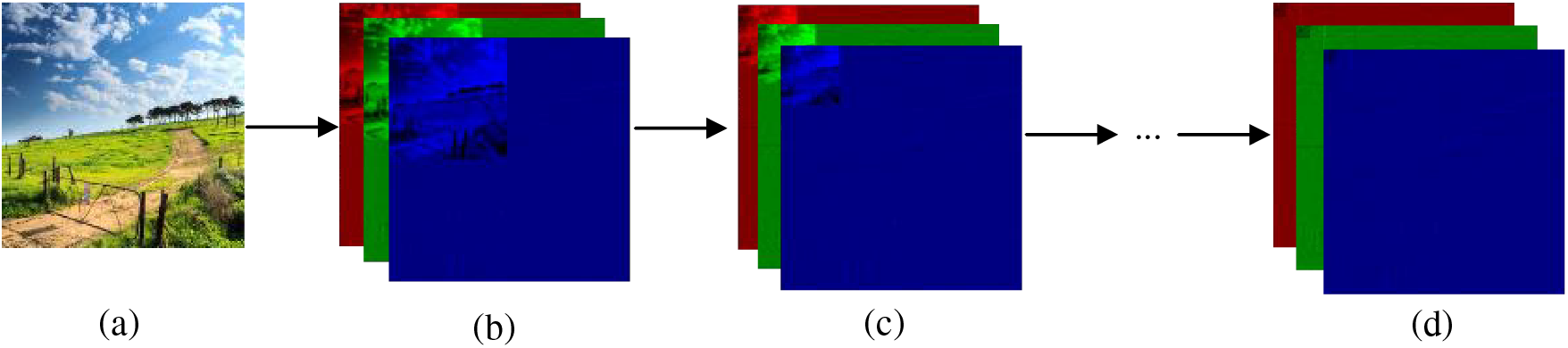
Figure 1: Preprocessing process: (a) A secret image of size 256 × 256; (b) The concatenated image of the four subbands from the first-level wavelet decomposition of the three channels of a secret image; (c) The concatenating image of four second-level decomposition subbands of the first-level approximation subband with three first-level detail subbands; (d) The approximation subband of the seventh-level decomposition is further decomposed into four subbands, which are concatenated with the previously obtained 21 subbands to form a 256 × 256 image

2.1.2 Dynamic Region Attention

In image hiding algorithms, regardless of whether the network is hidden or restored, the final result is related to the image’s quality and the algorithm’s security. The quality of an image is closely related to high-frequency areas and areas with strong color gradients, which often contain more detailed and edge information and are crucial to the overall visual quality and perception of the image. Establishing dynamic region attention can improve the quality of the network’s final output image.

Dynamic Region Attention (DRA) is an attention mechanism that dynamically adjusts the focus area of attention based on the characteristics of the input data. This method is particularly suitable for handling data with uneven distribution or multiple variations of crucial information, such as images, videos, and time series data. DRA enhances the model’s ability to recognize and utilize locally essential features in the data.

This study utilizes the spatial transformer network (STN) [35] to construct DRA based on high-frequency regions of images. DRA is divided into channel compression, attention weight, and element-wise multiplication. Channel compression compresses the extracted multi-channel features into a single channel. Attention weight is employed to obtain the attention weights of the compressed single channel. Element-wise multiplication is utilized to place the attention weights on the multi-channel features to enhance the locally essential features.

The complete process is shown in Fig. 2. The entire attention module has two branches that will eventually converge and output together. The multi-channel features are compressed into single-channel features via channel compression in the upper branch, and the high-frequency region weights are calculated. The final output is obtained after cross-channel integration through 1 × 1 convolution in the lower branch and element-wise multiplication with the obtained weights. The entire DRA focuses on obtaining the weights of region attention in the following process:

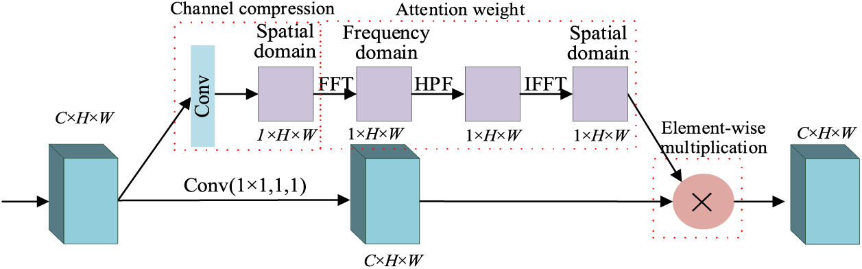
Figure 2: Structure of DRA module based on high-frequency image regions

(1)   Calculate the attention score: First, the extracted features are transformed from the spatial domain to the frequency domain by applying the Fourier transform—using a 2D Fast Fourier Transform (FFT) algorithm.

(2)   Suppress the low-frequency components and retain the high-frequency components using High-Pass Filtering (HPF).

(3)   Convert the filtered frequency domain image to the spatial domain using 2D Inverse Fast Fourier Transform (2D IFFT) to obtain the high-frequency components.

(4)   Generate the attention weight map: An attention weight map of the same size as the original image is constructed based on the intensity of the high-frequency components. Each pixel value in this attention weight map represents the importance of the corresponding pixel in the original image.

(5)   Standardization and Mapping. The obtained attention weight map is normalized to distribute the scores between 0 and 1, where 1 is the highest level of attention.

Finally, the weights of the features are obtained by integrating them into the model.

2.1.3 Dense Module

A DenseNet [36] is different from a ResCNN. The output of ResCNN is cumulative, which can hinder the flow of information in the network. However, DenseNet directly connects all inputs to the output layers. It consists of two main parts: dense blocks and transition layers. The dense block defines the relationship between input and output, while the transition layer controls the number of channels and shortens the connection between the front and back layers. DenseNet strengthens feature propagation, encourages feature reuse, and greatly reduces the number of parameters.

2.2 Structures of Image Hiding

The proposed hiding network consists of two parts: a feature extraction (the upper part in Fig. 3) and a container generation (the lower part in Fig. 3). The preprocessed secret image (S) and the carrier (C) are fed into the upper and lower parts, respectively. Three stacked convolutional layers extract features from the preprocessed secret image in the upper part. The extracted features are concatenated with the output of the third convolutional layer in the lower part and sent to the subsequent layers. To enhance the details of the container, in the lower part, the output of the first layer is concatenated with the outputs of the fourth, fifth, and sixth layers; the output of the second layer is concatenated with the outputs of the fifth and sixth layers; and the output of the third layer is concatenated with the output of the sixth layer. This operation is modeled after DenseNet, which uses dense connections and feature reuse to reduce the number of network parameters. Finally, the container image C* is obtained after two post-convolutional layers.

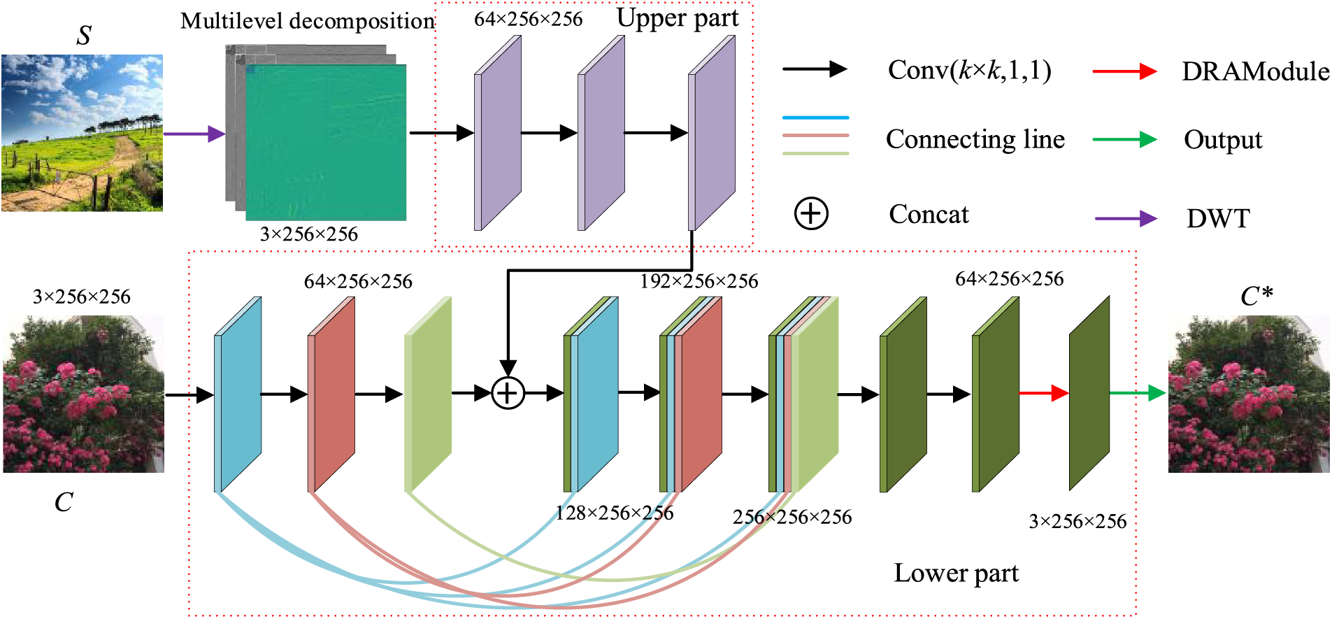
Figure 3: Structure of the hiding network

2.3 Recovery Network

The recovery network is structured as shown in Fig. 4 to extract the secret image from the container. The container image C* is evenly divided into four non-overlapping blocks (size 128 × 128 × 3) and sent to the four entrances of the recovery network. Each block contributes to the recovery of a small low-resolution secret image. The four branches of the recovery network have the same structure. After a three-layer convolution (Conv(3 × 3, 1, 1)), four feature maps of a quarter of the size of the original feature map are obtained. Then, after another special convolutional layer (Conv(4 × 4, 2, 2)), each of the four outputs is fed to the dense module. Next, the outputs of each of the four dense modules go to the convolutional layer and the DRA module at the same time. From top to bottom, as shown in Fig. 4, the output of the first DRA module is concatenated with the output of the fourth convolution layer; the output of the second DRA module is concatenated with the first convolution layer; the output of the third DRA module is concatenated with the output of the second convolutional layer; and the output of the fourth DRA module is concatenated with the output of the third convolution layer. Afterward, they pass through the convolutional layer and the pixel-shuffle layer successively. The pixel-shuffle layer enlarges the feature map by a factor of four and sends the output to the next dense module. Similarly, each output of the four dense modules arrives simultaneously at two places: the convolutional layer and the DRA module. The outputs of the four convolution layers are combined and sent to the convolutional layer. The output of the convolutional layer is concatenated with the outputs of the four DRA modules and then successively passes through the convolutional layer, the pixel-shuffle layer, and the dense module. Finally, the recovered secret image S* is obtained.

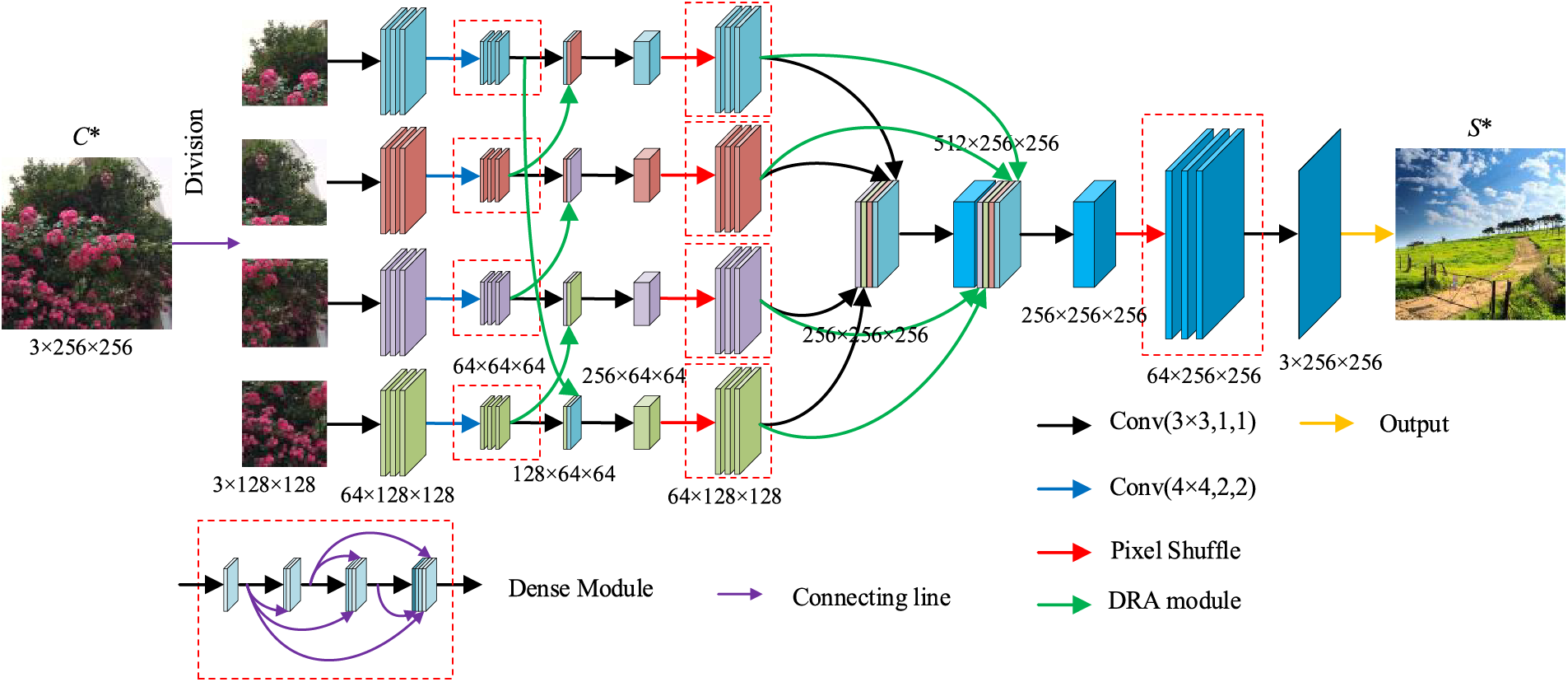
Figure 4: Structure of the recovery network

3  Dataset and Loss Function

3.1 Developmental Environment and Dataset

The hiding algorithm proposed in this study was implemented based on PyTorch 1.11.0 and trained using two GeForce RTX 3090Ti GPUs. Sixty thousand images from BOSSBase 1.01 [37] were used. This study resized all the original images to 256 × 256 and organized the 50,000 images into the training, validation, and test sets in a 4:1:1 ratio by random partitioning.

3.2 Training Process

During the training process, the loss function combines pixel and texture loss to restrict the container and reconstruct secret images.

3.2.1 Pixel Loss

The pixel loss between two images is defined as follows:

Lpixel=1cHW∑k=1c∑i=1H∑j=1W(y^i,j,k−yi,j,k)2(1)

where c is the number of channels of the image, typically 3; H is the height of the image; W is the image’s width; y^i,j,k is the pixel value of the image to be evaluated; yi,j,k is the pixel value of the reference image.

3.2.2 Texture Loss

Gatys et al. [38,39] introduced texture loss into super-resolution reconstruction to improve the texture similarity between the recovered and target images. For a color image I, let its Gram matrix be given as G∈ℜc×c, so its element at location (i, j) is defined as follows:

∑IGi,j(I)=Fi(I)Fj(I)(2)

where Fi(I) and Fj(I) are the i-th and j-th channels (R, G or B) of I, respectively. The expression for the texture loss of image y^ for y is as follows:

Ltexture=1c2∑i=1c∑j=1c(Gi,j(y^)−Gi,j(y))2(3)

For a color RGB format image, c = 3.

3.2.3 The Total Loss Function

During the training process, the hiding and recovery networks were trained together and constrained by the loss function. The loss function consists of two parts: the loss function LH for the hiding network and the loss function LR for the recovery network. The carrier image C and the secret image are the inputs of the hiding network, and the output of the hiding network is the container image C∗, as shown in Fig. 4. LH is utilized to minimize the difference between the carrier image C and the container image C∗, and is defined as follows:

LH=(Lpixel+Ltexture)/2=(13HW∑k=13∑i=1H∑j=1W(Ci,j,k∗−Ci,j,k)2+132∑i=13∑j=13(Gi,j(C∗)−Gi,j(C))2)(4)

where Ci,j,k∗,Ci,j,k are the pixel values at location (i, j) of the k-th channel of C∗ and C, respectively, in the first term; Gi,j(C∗) and Gi,j(C) are the Gram matrices of the i-th channel of C∗ and C, respectively.

LR is utilized to minimize the difference between the secret image S and the recovered secret image S∗, and it is defined as follows:

LH=(Lpixel+Ltexture)/2=(13HW∑k=13∑i=1H∑j=1W(Si,j,k∗−Si,j,k)2+132∑i=13∑j=13(Gi,j(S∗)−Gi,j(S))2)(5)

where Si,j,k∗,Si,j,k are the pixel values at location (i, j) of the k-th channel of S∗ and S, respectively.

Hence, the total loss function L is the sum of LH and LR.

L=LH+LR.(6)

During training, the batch size was set to 10, and the optimizer was chosen as Adam (Adaptive Moment Estimation) based on backpropagation. The initial learning rate was 0.015. The network training lasted over 25 days and converged after 1000 epochs, as shown in Fig. 5.

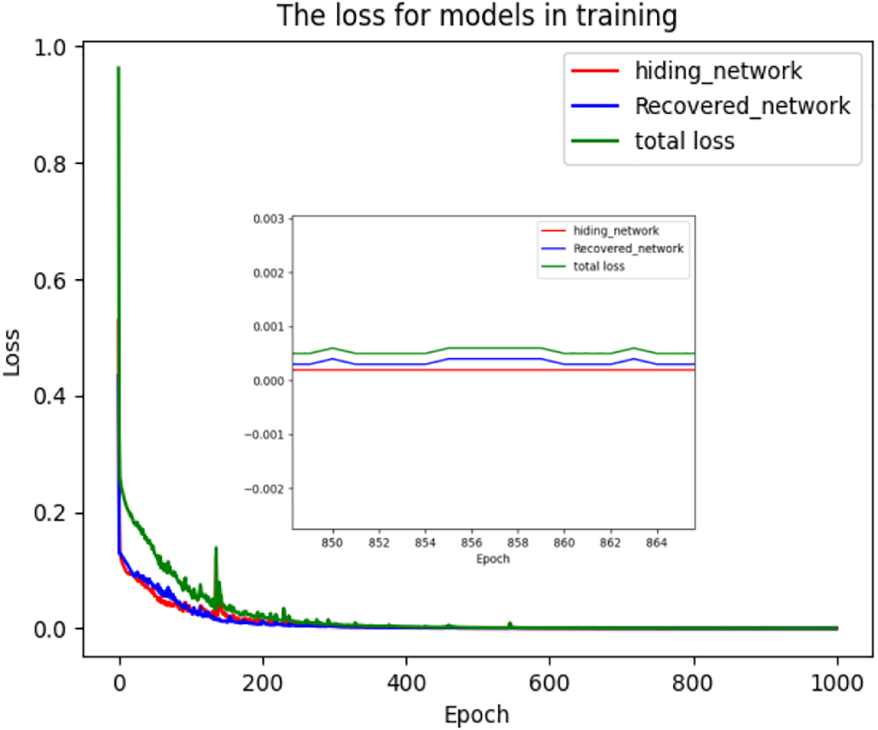
Figure 5: Loss function curves for the hiding network, recovery network, and total loss

Fig. 5 shows the relationship between the training epoch and the loss function. Fig. 5 indicates that the loss function LH decreases rapidly in the first 200 epochs and fluctuates in the following 400 epochs. It then enters a slow downward trend and converges to 0.001 after 600 epochs, eventually falling within the 0.0001–0.0002 interval. LR is similar to LH, converging to about 0.0005 after 600 epochs.

4  Experimental Results

This section shows the experimental results of the proposed hiding algorithm, including the performance of hiding and recovery.

4.1 Performance of the Hiding Algorithm

The four test image groups containing carrier images, secret images, container images, and corresponding recovered secret images and their difference images magnified by a factor of 20 are shown in Fig. 5. Fig. 6 indicates that the container images differ very little from their corresponding carrier images. In particular, the pixel values of the difference images between the carrier and container images remain small after being magnified by a factor of 20, and no abnormal disturbances can be visually perceived. Similarly, the differences and disturbances between the original secret and the recovered secret images are minimal, e.g., the whiskers of the recovered jellyfish are visible. Even when their different images are magnified 20 times, the outlines are only faintly visible.

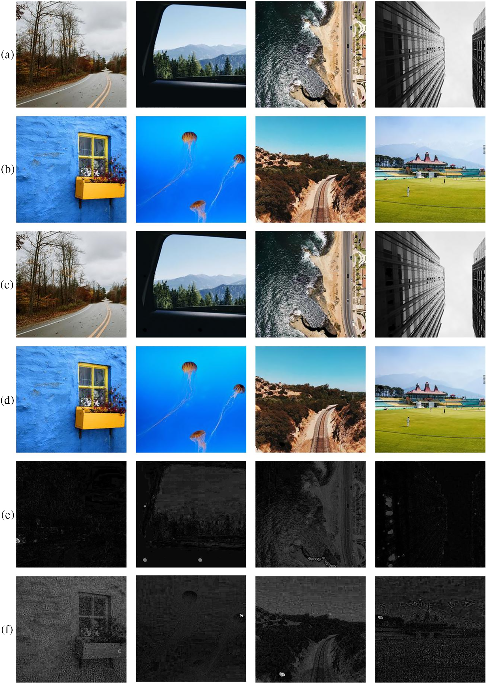
Figure 6: Steganography results: (a) carrier images; (b) secret images; (c) container images; (d) recovered secret images; (e) |a–c| × 20; (f) |b–d| × 20

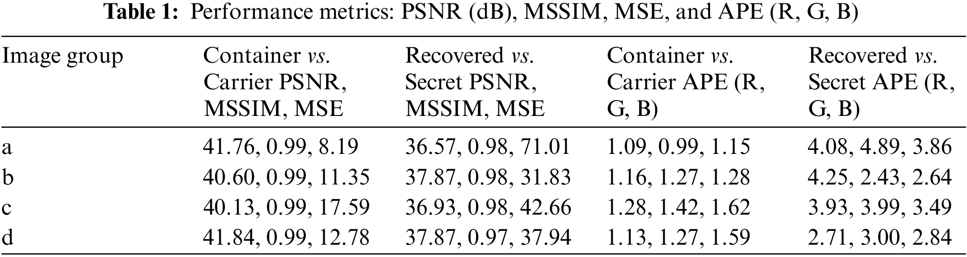
The evaluation metrics of the four test images in Fig. 6 are calculated and listed in Table 1 to illustrate the performance of the proposed steganography algorithm. The evaluation metrics include mean square error (MSE), peak signal-to-noise ratio (PSNR) [34], mean structural similarity (MSSIM) [40], and average absolute pixel error (APE) [27]. Table 1 shows that image groups a, b, c, and d correspond to the first, second, third, and fourth columns in Fig. 5. It exhibits that the PSNR between the container and carrier images exceeds 40 dB, and the MSSIM value reaches up to 0.99. This indicates that the image quality of the container images is excellent and very similar to that of the carrier image. The PSNR of the corresponding secret image exceeds 36 dB, and the MSSIM reaches 0.96, with a maximum APE of less than 5. This shows that the distortion of the recovered secret images is minimally acceptable.

4.2 Performance of Resistance to Noise Attacks

In the transmission process, the quality of the container image is often degraded due to the interference of various noises, adversely affecting subsequent image processing and visual effects. The effectiveness of recovering a high-quality secret image from a noise-polluted container is an index for evaluating steganography algorithms. In this section, the Gaussian noise with different intensities and the salt-and-pepper noise are added to the container image to demonstrate the restoration effect of the recovery network.

Fig. 7 shows container images with different Gaussian noise intensities, the corresponding recovered secret images, and their magnified detail images. Visually, the recovery network can reconstruct the ideal secret image when the container image is attacked by Gaussian noise. Most details are recovered, but the graininess and stereoscopic sense are lost. In addition, the quality of the recovered secret images does not decline rapidly with the increase in noise intensity. Table 2 indicates that when the Gaussian noise intensity is increased from 0.01 to 0.2 dBW (a 20-fold increase), the PSNR only decreases from 28.33 to 25.20 dB, while the MSSIM remains almost unchanged, with the APE and MSE increasing by factors of 2 and 3, respectively. This change is much smaller than the 20-fold change in the noise intensity. Even when the corresponding details of the recovered secret image are magnified by a factor of 9 (the edge length of the selected part is 1/3 of the original image), no noticeable difference can be observed. Only a minimal difference in color saturation is perceptible, and the edges become blurred.

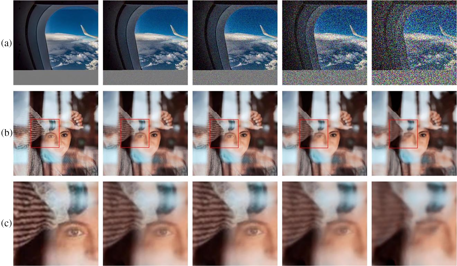
Figure 7: Steganography results when the container image is polluted by Gaussian noise of different intensities of 0, 0.01, 0.05, 0.1, and 0.2 dBW from left to right: (a) container image; (b) recovered secret images; (c) magnified with the corresponding details in (b) (enclosed area in the red rectangle)

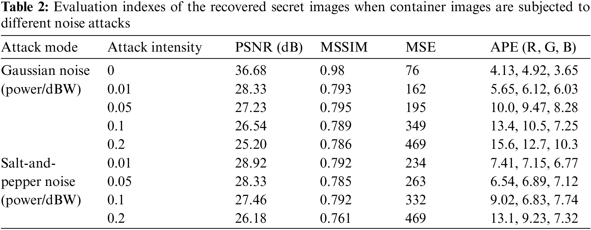
Fig. 8 exhibits container images with different salt-and-pepper noise intensities, the corresponding recovered secret images, and their magnified detail images. Similar to the case of Gaussian noise, the recovery network can reconstruct the ideal secret image, and the quality does not decline significantly with increasing noise intensity. Most of the details are recovered. Visually, there is no apparent difference between the original and recovered secret images at different noise intensities. This can also be verified with the quantitative results in Table 2. Table 2 indicates that when the salt-and-pepper noise intensity is increased from 0.01 to 0.2 dBW, the PSNR decreases from 28.92 to 26.18 dB, while the MSSIM remains almost unchanged, with no change in the APE and MSE increasing by less than twice their initial values. This change is far less than a 20-fold change in noise intensity. Similarly, no noticeable difference is observed when the corresponding details of the recovered secret image are magnified by a factor of 9. Only a minimal difference in color saturation is perceptible, and the edges become slightly blurred.

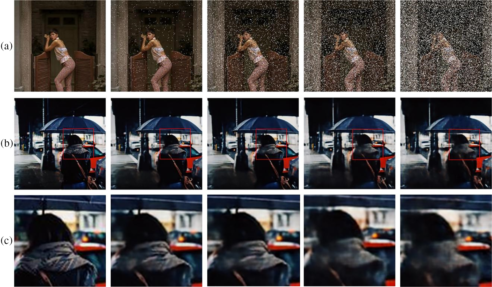
Figure 8: Steganography results when the container image is polluted with salt-and-pepper noise of different intensities of 0, 0.01, 0.05, 0.1, and 0.2 dBW from left to right: (a) container image; (b) recovered secret images; (c) magnified with the corresponding details in (b) (enclosed area in the red rectangle)

To summarize, the image quality of the container and the recovered secret images slowly decline if the intensity of Gaussian noise and salt-and-pepper noise gradually increases. However, the recovery network can effectively resist these two kinds of noise attacks and reconstruct the secret images with an acceptable quality.

4.3 Performance of Resistance to Cropping and Compression Attacks

Cropping and compression attacks are other common attacks that cause partial image data loss. They are often employed to test the robustness of steganography algorithms. The reconstruction effects of container images under different cropping and compression attacks are shown in Figs. 9 and 10.

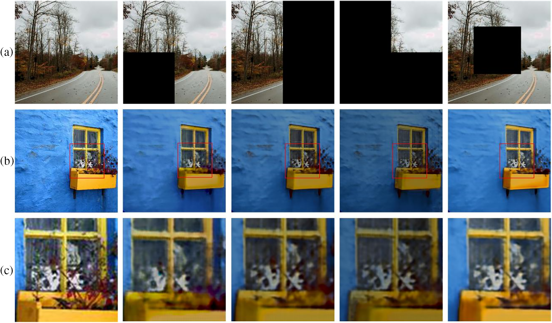
Figure 9: Steganography results when cropping the container image at different ratios of 0, 1/4, 1/2, 3/4, and 1/4 (center) from left to right: (a) container image; (b) recovered secret images; (c) magnified corresponding details in (b) (enclosed area in the red rectangle)

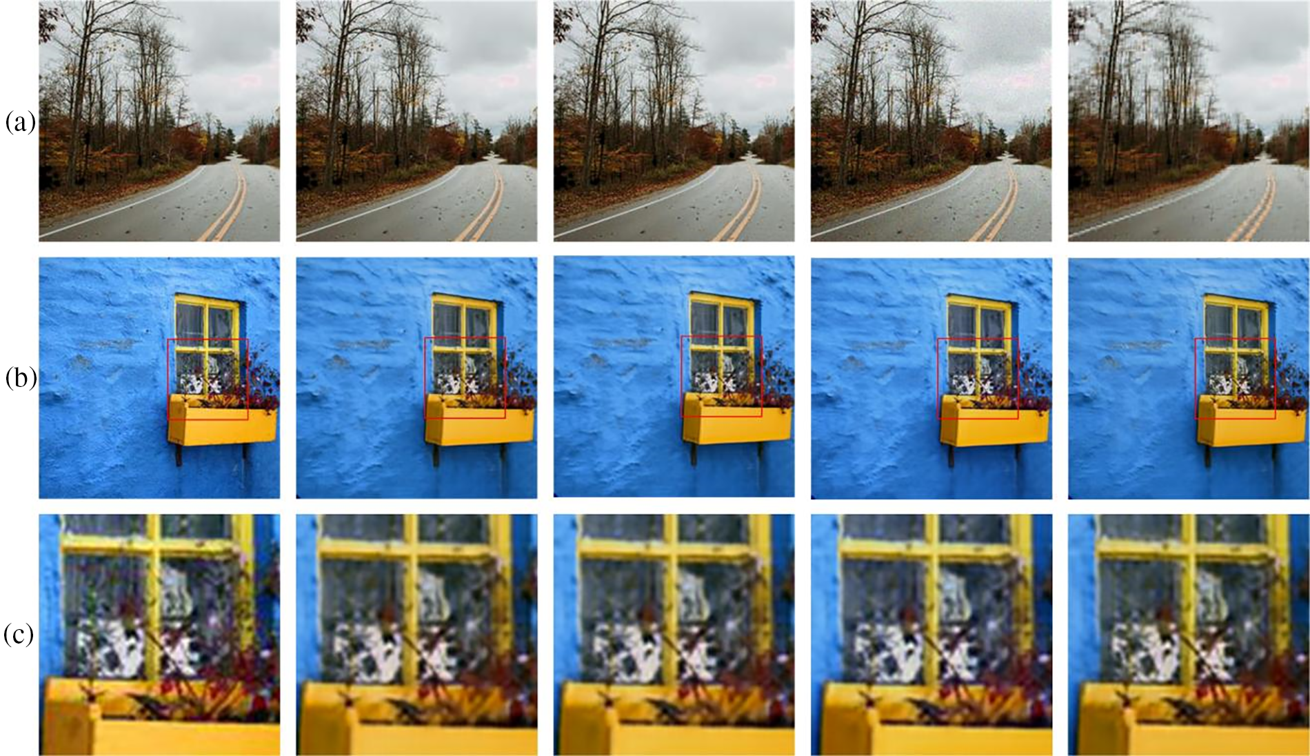
Figure 10: Steganography results when the container image is compressed with different ratios of 1, 1.18, 1.4, 2.2, and 5.8 from left to right: (a) container image; (b) recovered secret images; (c) magnified corresponding details in (b) (enclosed area in the red rectangle)

Fig. 9 shows the different cropping positions in the container, the corresponding recovered secret images, and their magnified detail images. As shown in the first row of Fig. 9, the container image is cut at a ratio of 0, 1/4, 1/2, 3/4, and 1/4 (center), respectively. As shown in the second row of Fig. 9, the color of the first four recovered secret images becomes increasingly unsaturated as the cropping size increases and the quality drops rapidly. The last one is cropped in the center area of the container at a ratio of 1/4, and the quality of the recovered image is the same as that of the second one, with the same cropping ratio, but in the left-bottom location. Visually, these recovered images only have a small difference in brightness and negligible difference in detail. This can also be verified by the quantitative results in Table 3. Table 3 indicates that when the cropping area size increases, the PSNR decreases from 21.86 to 14.21 dB, and the MSSIM decreases to as low as about 0.6. This shows that the structure of several secret recovered images has undergone some changes after cropping. However, due to the difference in pixel values, the PSNR reduces rapidly. In addition, the MSE and APE increase a lot with the increase of the cutting area. The secret image recovered from the partial container image can still contain much information about the secret image. Hence, when the container image is subjected to a cropping attack, acceptable secret images can still be recovered as long as enough container images are retained.

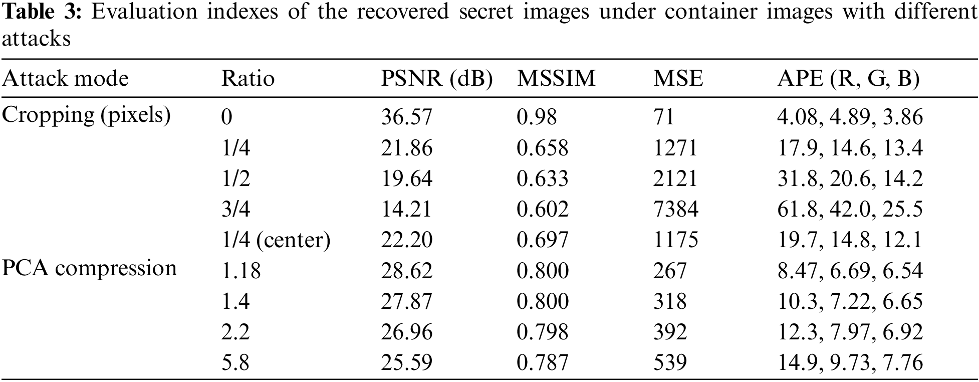
Fig. 10 shows the reconstruction results of container images with different compression ratios. The container is compressed using the principal component analysis (PCA) compression algorithm and then decompressed. The compression reduces the redundant information in the container image data, which decreases the quality of the recovered secret image. When the compression ratio is too large, the brightness of the recovered image diminishes. The results in Table 3 show the relationship between the quality of the recovered secret images and the compression ratios. As the compression ratio increases from 1.18 to 5.8, the PSNR between the recovered and original secret images decreases from 28.62 to 25.59 dB, and the MSSIM decreases from 0.8 to 0.787. At the same time, the MSE increases by about two times, from 267 to 539.

In summary, the proposed image steganography algorithm resists cropping and compression attacks.

4.4 Visual Comparison of DRA Modules

The proposed DRA module is applied in both hiding and recovery networks. The feature maps before and after the module are visualized and compared to illustrate the role of the module, as shown in Figs. 11 and 12.

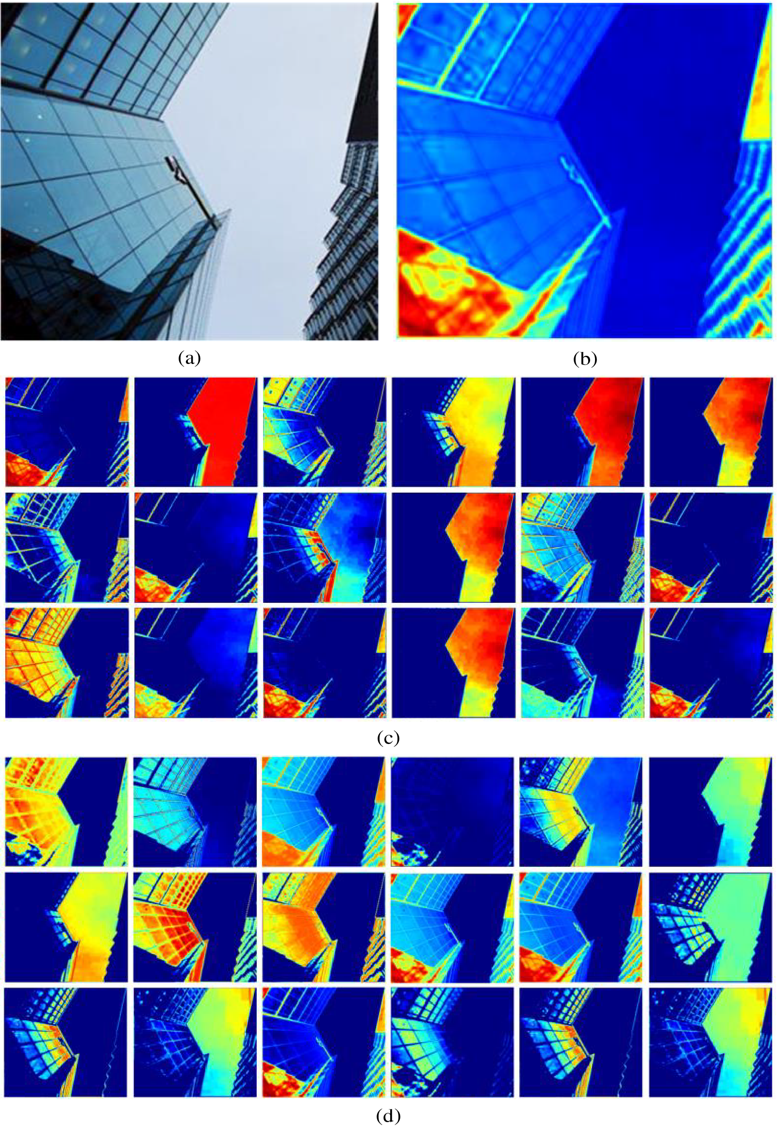
Figure 11: The performance of DRA modules in hiding networks: (a) container; (b) the weights of the features; (c) feature maps before using the DRA module; (d) feature map after using the DRA module

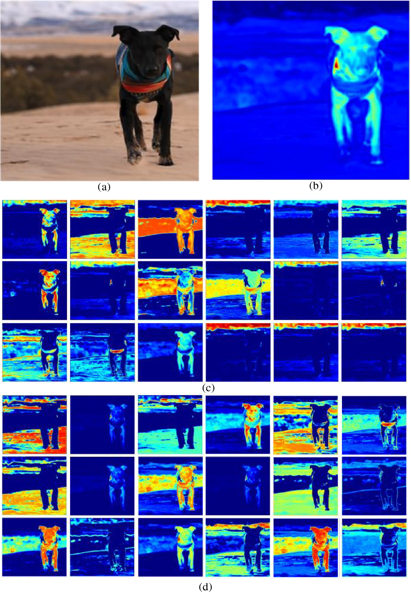
Figure 12: The performance of DRA modules in recovery networks: (a) recovered; (b) the weights of the features; (c) feature maps before using the DRA module; (d) feature map after using the DRA module

From Figs. 13 and 14, the changes in the features before and after applying the DRA module can be observed. The details in the features are significantly enhanced after the DRA operation.

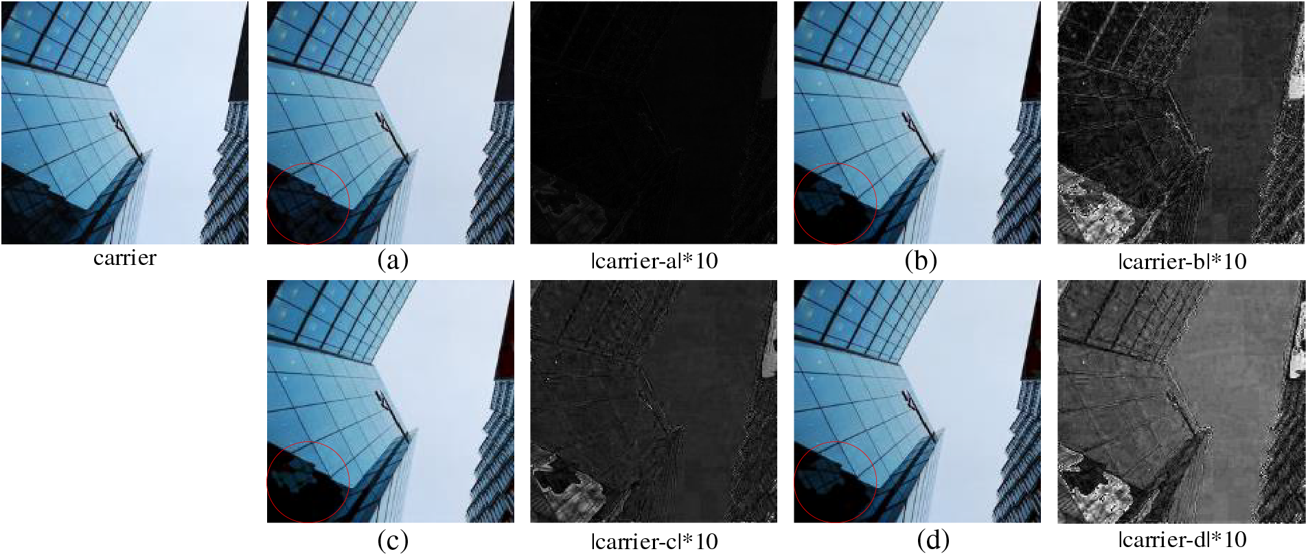
Figure 13: Visualization results displaying ablation experiments in the hiding network

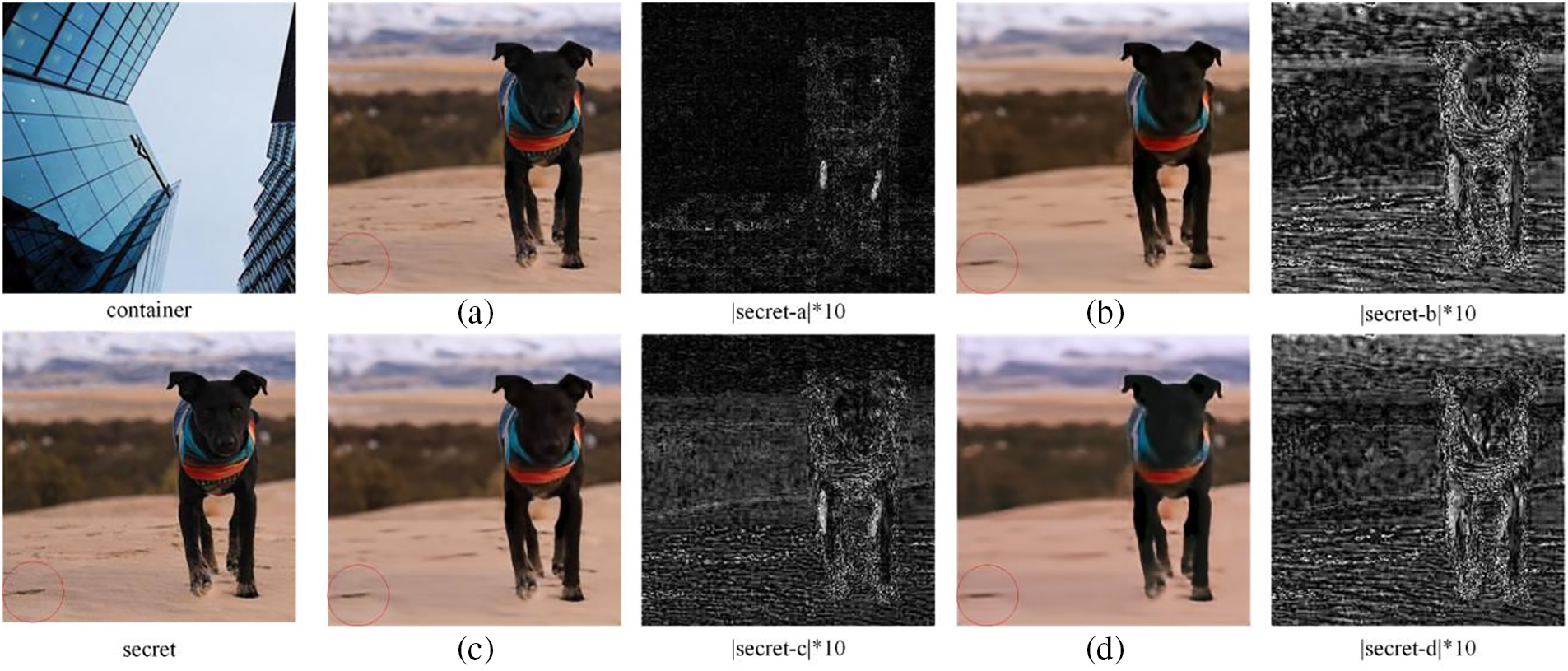
Figure 14: Visualization results displaying ablation experiments in the recovery network

4.5 Ablation Experiments

These two modules are replaced with modules usually connected to the recovery network to illustrate the role of the DenseNet and DRA modules in the recovery network. The check marks in Table 4 show the use of this structure in the network, and the cross marks indicate removal, resulting in three simplified networks. The three simplified recovery networks were trained the same number of times, 1000, and the trained model was saved. The trained simplified network models randomly selected and recovered one hundred container images.

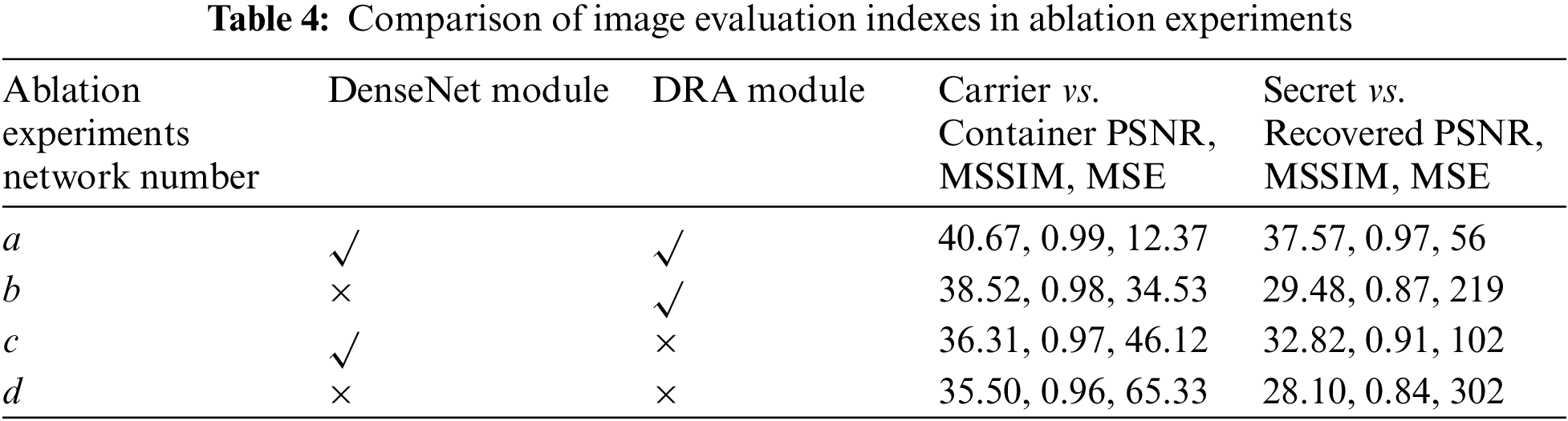
The results of one ablation experiment were randomly selected, as shown in Figs. 13 and 14. Fig. 13a–d corresponds to the containers produced by networks a–d in Table 4, with network a representing the proposed hiding network. The first column of the figure represents the carrier image, while the third and fifth columns represent the 10-fold difference between the carrier image and the container image, respectively. Similarly, Fig. 14a–d represents the recovered secret images by networks a–d in Table 4, with network a as the proposed recovery network. The first column in the figure represents the container image and the secret image, while the third and fifth columns represent the 10-fold difference between the recovered secret image and the original secret image, respectively. From the part circled in red, as the DenseNet and DRA modules are removed, the container and recovered secret images continue to deteriorate, as indicated by the different images.

The average image quality calculated for the recovered secret images is listed in Table 4. When the DenseNet module is deleted, the parameters and training time remain the same, but the quality of the container and recovered secret images is much lower than that of the complete network. The DenseNet module enables the extracted features to be reused without adding parameters, effectively improving the network’s expressive capability. When DRA modules are deleted, the parameters and training time are reduced, but the details of the recovered secret image become blurred. The role of the DRA module is to target key areas and details for focused enhancement so that the container and recovered images have better quality.

4.6 Resistance to Steganalysis

The effectiveness of a steganography algorithm in resisting steganalysis attacks is closely related to its other kinds of security. Three widely used open-source steganalysis algorithms, namely spatial rich model (SRM) [41], MaxSRM [42], and Ye-Net [43], were employed for testing. SRM is a spatially enriched model-based steganalysis method, mainly used for steganalysis of spatially coded images. SRM adopts multiple sub-models to extract more features and information about how steganography destroys multiple correlations of neighboring pixels. MaxSRM uses all the pixels of an image to calculate the sum of the maximum value of the embedded changes and the probability of the corresponding residuals to detect if this is a suspicious image. These two methods occupy the mainstream position in the traditional way of manual feature extraction. Ye-Net is based on the CNN steganography analysis model. It utilizes 30 filters of residual mapping in SRM as the weights of CNN to calculate the noise residuals, which can accelerate the network convergence. Three thousand images (1500 carrier and 1500 container ones) generated by the proposed steganography algorithm were used for steganalysis. The results are shown in Fig. 14, including receiver operating characteristic (ROC) curves and areas under the ROC curves (AUC) obtained by three steganalysis methods.

The image hiding algorithm proposed in this study uses a multi-level wavelet transform to decompose secret images. The low-frequency component degenerates into a single coefficient in the wavelet domain. This reduces the variance of the adjacent pixel correlation of container images, making those traditional steganalysis algorithms useless. Fig. 15 indicates that the AUCs of SRM and MaxSRM are 0.51 and 0.52, respectively, slightly higher than a random guess. Ye-Net also improved the accuracy of discrimination only to 0.58. This shows that the proposed steganography model resists traditional and deep learning-based image steganalysis.

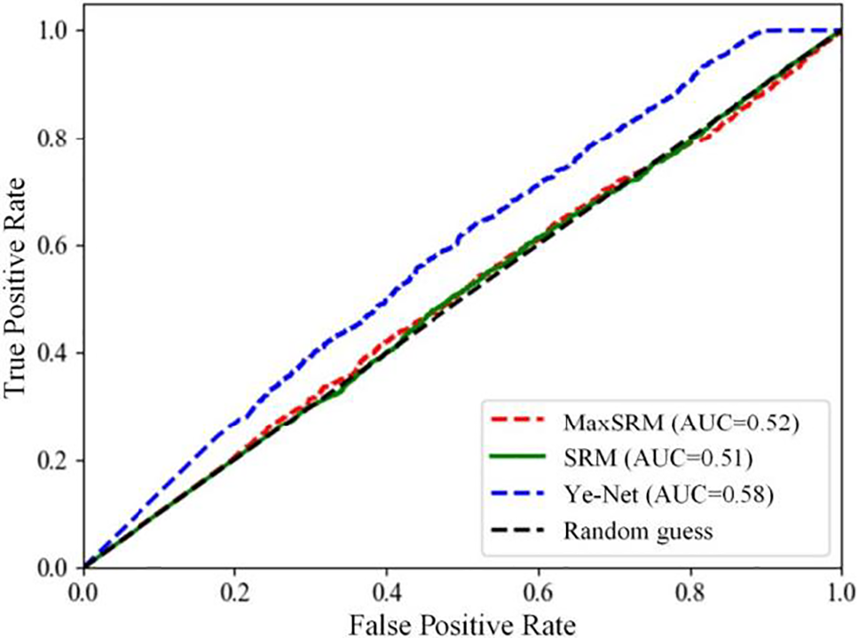
Figure 15: ROC and AUC were obtained using three steganalysis algorithms

4.7 Comparison with Other State-of-the-Art CNN Steganography Approaches

This section compares the proposed steganography with other state-of-the-art CNN approaches regarding image hiding and recovery performance and the performance against steganography analysis. The comparative results are shown in Table 5, representing the averages for 100 groups of container and carrier images.

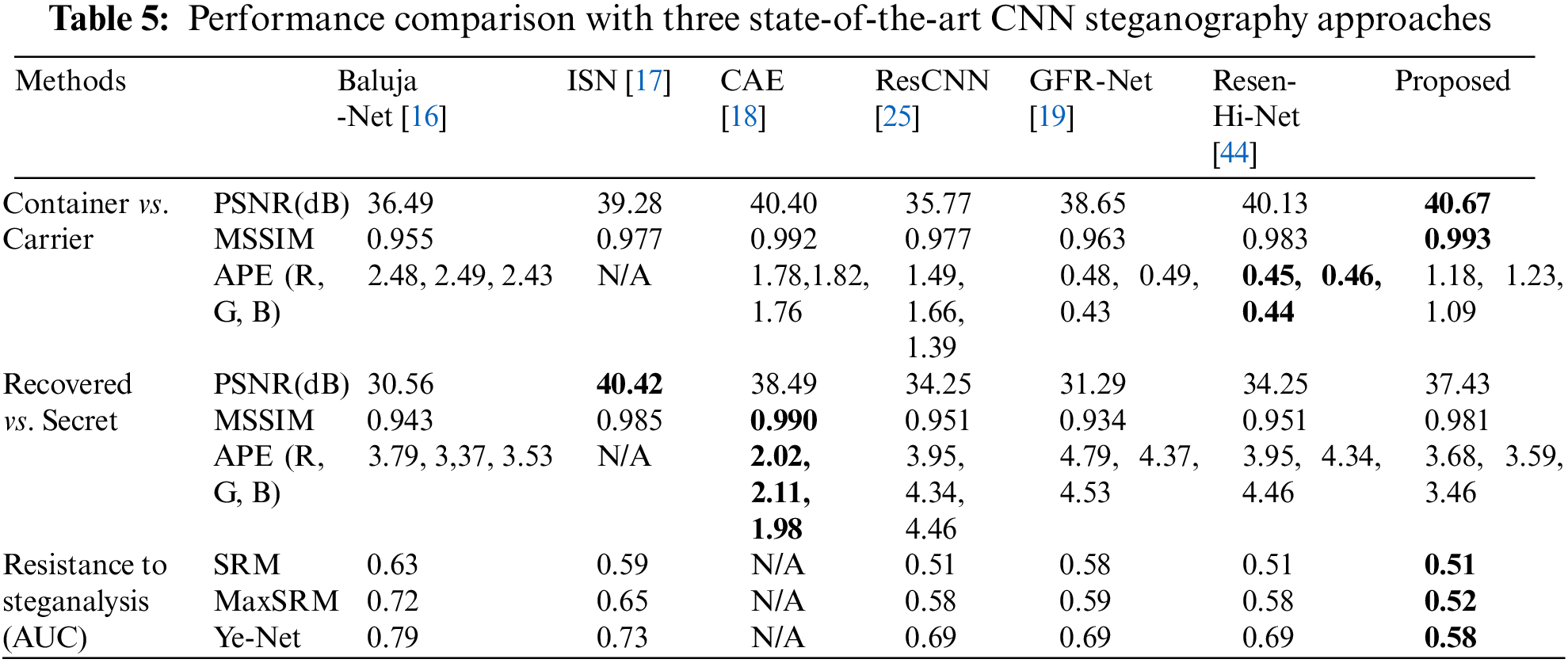
Table 5 indicates that PSNR and MSSIM reached the optimum, but APE was not the best. This is because the model training employed a joint constraint of pixel loss and texture loss. Although a simple pixel loss constraint can reduce the value of APE, it also affects the PSNR and MSSIM. As a result, texture loss was introduced to improve the PSNR and MSSIM of the container image and recovered secret images. The PSNR and MSSIM of the container image were optimal, resulting in the best resistance to steganalysis. However, the PSNR and MSSIM of the recovered secret image were suboptimal, slightly lower than those of ISN, with little deviation from the APE. Hence, the proposed steganography algorithm outperforms the others.

5  Conclusion and Discussion

A new image hiding algorithm with high robustness is proposed. Through wavelet multi-scale decomposition, the low-frequency component of the secret image degenerates into a single coefficient in the wavelet domain, which improves the security and resistance against steganalysis algorithms. The recovery process divides the container image into four non-overlapping quarter-sized sub-images. Each sub-image hides partial information about the secret image and can be used to reconstruct low-resolution secret images. High-quality secret images can be obtained by concatenating and reconstructing the features of secret images extracted from the four sub-containers. Compared to other CNN image hiding algorithms, due to the embedding features, the proposed hiding algorithm is effective in resisting various hiding analysis attacks and highly robust when container images are subject to destructive attacks such as noise, cropping, and compression attacks.

Acknowledgement: None.

Funding Statement: This work was partly supported by the National Natural Science Foundation of China (Jianhua Wu, Grant No. 62041106).

Author Contributions: The authors confirm their contribution to the paper as follows: Xishun Zhu, Donghua Jiang and Jianhua Wu proposed the hiding algorithm, Zengxiang Li, Jianhua Wu and Yongchong Wu implemented algorithm through programming, Yongchong Wu, Donghua Jiang and Alanoud Al Mazroa conducted experiments based on the algorithm, Zengxiang Li, Alanoud Al Mazroa and Donghua Jiang wrote the main manuscript text, Zengxiang Li and Yongchong Wu prepared figures and tables. All authors reviewed the results and approved the final version of the manuscript.

Availability of Data and Materials: The data used in the article can be accessed at: http://agents.fel.cvut.cz/boss/index.php?mode=view&tmpl=materials (accessed on 30 April 2024).

Conflicts of Interest: The authors declare that they have no conflicts of interest to report regarding the present study.

References

1. Liu Z, Chen H, Blondel W, Shen Z, Liu S. Image security based on iterative random phase encoding in expanded fractional Fourier transform domains. Opt Laser Eng. 2018;105:1–5. doi:10.1016/j.optlaseng.2017.12.007. [Google Scholar] [CrossRef]

2. Liu Z, Li S, Yang M, Liu W, Liu S. Image encryption based on the random rotation operation in the fractional Fourier transform domains. Opt Laser Eng. 2012;50(10):1352–8. doi:10.1016/j.optlaseng.2012.05.021. [Google Scholar] [CrossRef]

3. Mielikainen J. LSB matching revisited. IEEE Signal Proc Let. 2006;13(5):285–7. doi:10.1109/LSP.2006.870357. [Google Scholar] [CrossRef]

4. Li X, Yang B, Cheng D, Zeng T. A generalization of LSB matching. IEEE Signal Proc Let. 2019;16(2):69–72. [Google Scholar]

5. Fridrich J, Kodovský J. Multivariate Gaussian model for designing additive distortion for steganography. In: IEEE International Conference on Acoustics, Speech and Signal Processing; 2013; Vancouver, BC, Canada. p. 2949–53. [Google Scholar]

6. Sedighi V, Cogranne R, Fridrich J. Content-adaptive steganography by minimizing statistical detectability. IEEE T Inf Foren Sec. 2015;11(2):221–34. doi:10.1109/TIFS.2015.2486744. [Google Scholar] [CrossRef]

7. Filler T, Judas J, Fridrich J. Minimizing additive distortion in steganography using syndrome-trellis codes. IEEE T Inf Foren Sec. 2011;6(3):920–35. doi:10.1109/TIFS.2011.2134094. [Google Scholar] [CrossRef]

8. Holub V, Fridrich J, Denemark T. Universal distortion function for steganography in an arbitrary domain. Eurasip J Inform Secur. 2014;1(1):1–13. doi:10.1186/1687-417X-2014-1. [Google Scholar] [CrossRef]

9. Li B, Ming W, Huang J, Li X. A new cost function for spatial image steganography. In: IEEE International Conference on Image Processing; 2014; Paris: France. p. 4204–10. [Google Scholar]

10. Holub V, Fridrich J. Designing steganographic distortion using directional filters. In: IEEE Workshop on Information Forensic and Security; 2012; Tenerife, Spain. p. 234–9. [Google Scholar]

11. Pevný T, Filler T, Bas P. Using high-dimensional image models to perform highly undetectable steganography. In: 12th Information Hiding Workshop; 2010; Calgary, AB, Canada. p. 161–77. [Google Scholar]

12. Goodfellow I, Bengio Y, Courville A. Deep learning. Cambridge, MA, USA: MIT press; 2016. vol. 1, p. 326–66. [Google Scholar]

13. Gu J, Wang Z, Kuen J, Ma L, Shahroudy A, Shuai B, et al. Recent advances in convolutional neural networks. Pattern Recogn. 2018;77(11):354–77. doi:10.1016/j.patcog.2017.10.013. [Google Scholar] [CrossRef]

14. Rehman AU, Rahim R, Nadeem MS, Hussain SU. End-to-end trained CNN encode-decoder networks for image. In: European Conference on Computer Vision Workshops; 2018; Munich, Germany. p. 723–9. [Google Scholar]

15. Subramanian N, Cheheb I, Elharrouss O, Al-Maadeed S, Bouridane A. End-to-end image steganography using deep convolutional autoencoders. IEEE Access. 2021;9:135585–93. doi:10.1109/ACCESS.2021.3113953. [Google Scholar] [CrossRef]

16. Baluja S. Hiding images within images. IEEE T Pattern Anal. 2020;42(7):1685–97. doi:10.1109/TPAMI.2019.2901877. [Google Scholar] [PubMed] [CrossRef]

17. Lu S, Wang R, Zhong T, Paul LR. Large-capacity image steganography based on invertible neural networks. In: IEEE/CVF Conference on Computer Vision and Pattern Recognition; 2021. p. 10816–25. [Google Scholar]

18. Liu X, Ma Z, Guo X, Hou J, Wang L, Zhang J, et al. Joint compressive autoencoders for full-image-to-image hiding. In: International Conference on Pattern Recognition; 2021; Milan, Italy. p. 7743–50. [Google Scholar]

19. Wu J, Lai Z, Zhu X. Generative feedback residual network for high-capacity image hiding. J Mod Optic. 2022;69(13/15):870–86. [Google Scholar]

20. Wu P, Yang Y, StegNet Li X. Megaimage steganography capacity with deep convolutional network. Future Int. 2018;10(6):64. [Google Scholar]

21. Duan X, Jia K, Li B, Guo D, Zhang E, Qinet C. Reversible image steganography scheme based on a U-Net structure. IEEE Access. 2019;7(1):9314–23. doi:10.1109/ACCESS.2019.2891247. [Google Scholar] [CrossRef]

22. He K, Zhang X, Ren S, Sun J. Deep residual learning for image recognition. In: IEEE Conference on Computer Vision and Pattern Recognition; 2016; Las Vegas, NV, USA. p. 770–8. [Google Scholar]

23. Wang G, Zeng G, Cui X, Feng S. Dispersion analysis of the gradient weighted finite element method for acoustic problems in one, two, and three dimensions. Int J Numer Meth Eng. 2019;120(4):473–97. doi:10.1002/nme.6144. [Google Scholar] [CrossRef]

24. Duan X, Li B, Xie Z, Yue D, Ma Y. High-capacity information hiding based on residual network. ITET Technical Review. 2021;38(1):172–83. doi:10.1080/02564602.2020.1808097. [Google Scholar] [CrossRef]

25. Zhu X, Lai Z, Liang Y, Xiong J, Wu J. Generative high-capacity image hiding based on residual CNN in wavelet domain. Appl Soft Comput. 2021;115:108170. [Google Scholar]

26. Mallat S. A compact multiresolution representation: the wavelet model. In: IEEE International Conference on Computer Vision; 1987. London, UK. p. 2–7. [Google Scholar]

27. Mallat S. The theory for multiresolution signal decomposition: the wavelet representation. IEEE T Pattern Anal. 1989;11(7):654–93. doi:10.1109/34.192463. [Google Scholar] [CrossRef]

28. Varuikhin V, Levina A. Continuous wavelet transform applications in steganography. Procedia Comput Sci. 2021;186(1):580–7. doi:10.1016/j.procs.2021.04.179. [Google Scholar] [CrossRef]

29. Pandimurugan V, Sathish K, Amudhavel J, Sambath M. Hybrid compression technique for image hiding using Huffman, RLE and DWT. Mater Today. 2022;57(5):2228–33. [Google Scholar]

30. Khandelwal J, Sharma VK, Singh D, Zaguia A. DWT-SVD based image steganography using threshold value encryption method. Comput Mater Contin. 2022;8(2):3299–312. doi:10.32604/cmc.2022.023116. [Google Scholar] [CrossRef]

31. Raju K, Nagarajan A. A steganography embedding method based on CDF-DWT technique for reversible data hiding application using elgamal algorithm. Int J Found Comput S. 2022;6(7):489–512. [Google Scholar]

32. Yue L, Shen H, Li J, Yuan Q, Zhang H, Zhang L. Image super-resolution: the techniques, applications, and future. Signal Process. 2016;128:389–408. [Google Scholar]

33. Li Q, Zhang A, Liu P, Li J, Li C. A novel CSI feedback approach for massive MIMO using LSTM-attention CNN. Access. 2020;8:7295–302. [Google Scholar]

34. Welstead S. Fractal and wavelet image compression techniques. In: Society of Photo-Optical Instrumentation Engineers (SPIE); 1999; WA, USA: SPIE Optical Engineering Press. p. 155–6. [Google Scholar]

35. Mo K. Spatial Transformer Network; 2016. Available from: https://arxiv.org/abs/1506.02025. [Accessed 2024]. [Google Scholar]

36. Iandola F, Moskewicz M, Karayev S, Girshick R, Keutzer K. Implementing efficient ConvNet descriptor pyramids; 2014. doi:10.48550/arXiv.1404.1869. [Google Scholar] [CrossRef]

37. Bas P, Filler T, Pevny T. Break our steganographic system: the ins and outs of organizing BOSS. In: 13th International Conference on Information Hiding; 2011; Prague, Czech Republic. p. 59–70. [Google Scholar]

38. Gatys L, Ecker A, Bethge M. Texture synthesis using convolutional neural networks; 2015. Available from: https://arxiv.org/abs/1505.07376. [Accessed 2024]. [Google Scholar]

39. Gatys L, Ecker A, Bethge M. Image style transfer using convolutional neural networks. In: IEEE Conference on Computer Vision and Pattern Recognition; 2016; Las Vegas, NV, USA. p. 2414–23. [Google Scholar]

40. Wang Z, Bovik A, Sheikh R, Simoncelli E. Image quality assessment: from error visibility to structural similarity. IEEE T Image Process. 2014;13:600–12. [Google Scholar]

41. Fridrich J, Kodovský J. Rich models for steganalysis of digital images. In: IEEE International Workshop on Information Forensics and Security; 2012; Tenerife, Spain. p. 868–82. [Google Scholar]

42. Denemark T, Sedighi V, Holub V, Cogranne R, Fridrich J. Selection-channel-aware rich model for steganalysis of digital image. In: IEEE International Workshop on Information Forensics and Security; 2014; Atlanta, GA, USA. p. 48–53. [Google Scholar]

43. Ye J, Ni J, Yi Y. Deep learning hierarchical representations for image steganalysis. In: IEEE International Workshop on Information Forensics and Security; 2017; Rennes, France. vol. 12, p. 2545–57. [Google Scholar]

44. Zhu X, Lai Z, Zhou N, Wu J. Steganography with high reconstruction robustness: hiding of encrypted secret images. Mathematics. 2022;10(16):10162934. doi:10.3390/math10162934. [Google Scholar] [CrossRef]