
 Submit a Paper
 Propose a Special lssue
 Open Access
ARTICLE

A Microseismic Signal Denoising Algorithm Combining VMD and Wavelet Threshold Denoising Optimized by BWOA
1 Zijin Mining Group Co., Ltd., Xiamen, 361016, China
2 Zijin (Changsha) Engineering Technology Co., Ltd., Changsha, 410006, China
3 State Key Laboratory of Comprehensive Utilization of Low-Grade Refractory Gold Ores, Shanghang, 364204, China
4 School of Resources and Safety Engineering, Central South University, Changsha, 410083, China
5 School of Resources & Environment Engineering, Jiangxi University of Science and Technology, Ganzhou, 341000, China
6 Zijin School of Geology and Mining, Fuzhou University, Fuzhou, 350116, China
7 State Key Laboratory for Fine Exploration and Intelligent Development of Coal Resources, China University of Mining and Technology, Xuzhou, 221116, China
* Corresponding Author: Zhi Yu. Email:
(This article belongs to the Special Issue: Bio-inspired Optimization in Engineering and Sciences)
Computer Modeling in Engineering & Sciences 2024, 141(1), 187-217. https://doi.org/10.32604/cmes.2024.051402
Received 05 March 2024; Accepted 14 June 2024; Issue published 20 August 2024
 View Full Text
 Download PDF
Abstract
The denoising of microseismic signals is a prerequisite for subsequent analysis and research. In this research, a new microseismic signal denoising algorithm called the Black Widow Optimization Algorithm (BWOA) optimized Variational Mode Decomposition (VMD) joint Wavelet Threshold Denoising (WTD) algorithm (BVW) is proposed. The BVW algorithm integrates VMD and WTD, both of which are optimized by BWOA. Specifically, this algorithm utilizes VMD to decompose the microseismic signal to be denoised into several Band-Limited Intrinsic Mode Functions (BLIMFs). Subsequently, these BLIMFs whose correlation coefficients with the microseismic signal to be denoised are higher than a threshold are selected as the effective mode functions, and the effective mode functions are denoised using WTD to filter out the residual low- and intermediate-frequency noise. Finally, the denoised microseismic signal is obtained through reconstruction. The ideal values of VMD parameters and WTD parameters are acquired by searching with BWOA to achieve the best VMD decomposition performance and solve the problem of relying on experience and requiring a large workload in the application of the WTD algorithm. The outcomes of simulated experiments indicate that this algorithm is capable of achieving good denoising performance under noise of different intensities, and the denoising performance is significantly better than the commonly used VMD and Empirical Mode Decomposition (EMD) algorithms. The BVW algorithm is more efficient in filtering noise, the waveform after denoising is smoother, the amplitude of the waveform is the closest to the original signal, and the signal-to-noise ratio (SNR) and the root mean square error after denoising are more satisfying. The case based on Fankou Lead-Zinc Mine shows that for microseismic signals with different intensities of noise monitored on-site, compared with VMD and EMD, the BVW algorithm is more efficient in filtering noise, and the SNR after denoising is higher.Keywords
Abbreviation
| VMD | Variational Mode Decomposition |
| BWOA | Black Widow Optimization Algorithm |
| WTD | Wavelet Threshold Denoising |
| BVW | The BWOA optimized VMD joint WTD Algorithm |
| EMD | Empirical Mode Decomposition |
| EEMD | Ensemble Empirical Mode Decomposition |
| BLIMF | Band-limited Intrinsic Mode Function |
| SNR | The signal-to-noise ratio |
| RMSE | The root mean square error |
| P-CC | The Pearson correlation coefficient |
| TFR | The time-frequency representation |
As mineral resources in the shallow earth gradually become exhausted, mining has gradually entered the deep earth. One of the accompanying problems is that ground pressure disasters occur more frequently, which will seriously threaten the safety of personnel and equipment. Therefore, the safety issue in deep underground mines has become a popular research topic [1,2]. As an efficient means of ground pressure monitoring, microseismic monitoring technology can be used for long-term, uninterrupted monitoring. This technology is effective in monitoring microfractures that may develop into macro instability failures inside rock masses and revealing the state of failure development in rock masses. By processing and analyzing microseismic records, engineering and technical personnel are able to get the precursor of ground pressure disaster, and take timely and reasonable measures, so as to protect personnel or equipment from the damage caused by ground pressure disasters and ensure safe and smooth production activities. Therefore, this technology has been extensively applied in mines [3,4].
The microseismic events that this paper focuses on are mining-induced microseismic events, whose main characteristics are similar to earthquakes [5,6], belonging to mechanical waves propagating in rock masses and exhibiting both the P-phases and S-phases. However, because its energy is small, the magnitude is generally less than 0, and the propagation distance is generally short, it often exhibits features of a low signal-to-noise ratio (SNR) and an overlap of the P- and S-phases [4]. Resulting from the complexities of underground construction environments and geological conditions, the signals acquired by microseismic monitoring systems usually contain various noises, including electrical signals, mechanical vibration signals, and drilling signals [7], whose frequency and amplitude can be distributed throughout the whole record, which greatly impacts follow-up analysis, such as picking the arrival time of P/S waves, parameter inversion, and mechanism analysis [4]. Therefore, denoising the microseismic signal monitored is essential for subsequent analysis and research.
Microseismic signals exhibit nonstationarity and randomness [8,9]. The commonly employed techniques for processing these signals involve Wavelet Threshold Denoising (WTD) [10], Empirical Mode Decomposition (EMD) [11], and the improved techniques derived from EMD, including Ensemble Empirical Mode Decomposition (EEMD) [12]. The foundation of WTD is wavelet transform. For example, Xu et al. [13] applied wavelet transform to denoise microseismic signals. They verified through experiments that the syml6 wavelet basis function is suitable for denoising microseismic signals monitored in large-scale rock structures and evaluated the denoising performance of four commonly used threshold algorithms, including the rigrsure threshold algorithm [14]. Their experiments indicate that the rigrsure threshold algorithm achieved the best SNR and root mean square error (RMSE), and its denoising was the most effective. However, WTD needs to determine multiple parameters, such as the threshold algorithm and the wavelet basis function. As a result, its denoising performance is affected by the mutual influence of harmonic components in every frequency band in the original signal [15], which makes qualitative analysis and research difficult to conduct. Moreover, this algorithm cannot filter out high-frequency noise [16], which affects the denoising performance. In 1998, Huang et al. [17] proposed the classic adaptive signal processing technique EMD, which exhibits excellent performance in processing non-stationary signals. This method decomposes the signal based on its time-scale characteristics to obtain several intrinsic mode functions. Then, each intrinsic mode function is analyzed and screened for signal reconstruction. In light of these benefits, the EMD method is extensively applied to microseismic signal denoising [18,19]. Nevertheless, EMD is deficient in a robust theoretical basis and is liable to experience mode mixing [20,21]. EEMD is an improvement based on EMD. This method involves adding Gaussian white noise to the signal beforehand, followed by mode decomposition. In this way, the process of adding different Gaussian white noise and then decomposition is repeated many times. Finally, the results of repeated processes are averaged to obtain more accurate intrinsic mode functions [12,22]. Although this improved method solves the issue of mode mixing in EMD, the iterative process increases the computational complexity of the algorithm, and errors may occur due to poor selection of the amplitude of pre-added Gaussian white noise and iteration times [23].
In addition, there are also some other methods used for denoising microseismic signals. For example, Dong et al. [24] proposed a denoising algorithm called LMD-SVD, which is a combination of Local Mean Decomposition and Singular Value Decomposition. In the algorithm, the signal is decomposed using Local Mean Decomposition and obtain several product functions from high to low frequencies. After screening, Singular Value Decomposition is used to denoise the low-frequency product functions, and the denoised signal is obtained after reconstruction. Li et al. [25] developed a microseismic signal denoising method combining Empirical Wavelet Transform and adaptive threshold. With this technique, the signal undergoes adaptive decomposition into distinct modes, guided by its frequency characteristics. Then, the modes containing more useful components are processed using the hard threshold function to preserve the amplitude, while other modes containing fewer useful components are processed using an improved threshold function to ensure the reconstructed signal remains continuous. Peng et al. [26] proposed a non-parametric automatic algorithm for denoising microseismic signals. This method first applies the two-step Akaike Information Criterion to pick up the arrival of P-waves. Then the noise power spectrum is subtracted from the signal power spectrum. Finally, the reconstructed signal is acquired through the inverse Fourier transform.
Variational Mode Decomposition (VMD) [27] is a modal variational and signal-processing algorithm introduced in 2014, which is characterized by self-adaptation and complete non-recursion. In VMD, the number of decomposed Band-Limited Intrinsic Mode Functions (BLIMFs) is capable of being manually set, and the finite bandwidth of BLIMFs and the optimal center frequency can be matched autonomously during the algorithm process. So mode separation is more effective, and mode mixing and other problems do not exist in VMD. When VMD is applied to complex nonlinear time series, it can effectively reduce nonstationarity, therefore, it has been thoroughly researched and utilized in the past few years [28]. However, its decomposition performance is usually affected by the number of BLIMFs K and the penalty factor
This study presents a novel algorithm for denoising microseismic signals. This algorithm is called the Black Widow Optimization Algorithm (BWOA) optimized VMD joint WTD algorithm, abbreviated as BVW. As shown in Fig. 1, in the algorithm, firstly, the microseismic signal is decomposed using VMD, and then the BLIMFs with correlation coefficients higher than the threshold are selected as the effective mode functions. Then, the residual low- and intermediate-frequency noise in the effective mode functions are filtered out through WTD. Finally, the denoised microseismic signal is obtained through reconstruction. The values of VMD parameters, including the number of BLIMFs K and penalty factor
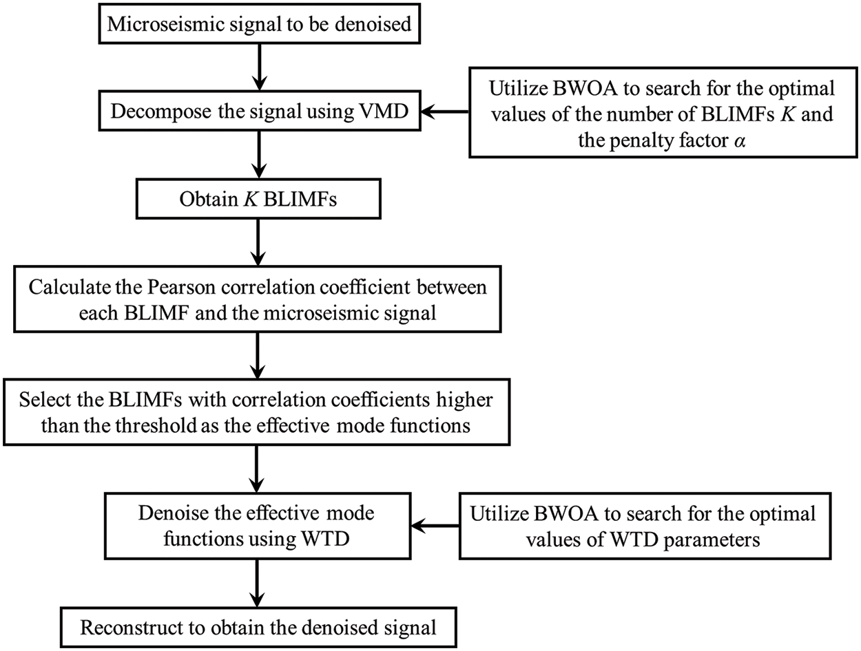
Figure 1: The schematic diagram of the BVW algorithm
2.1 The BWOA Optimized VMD Joint WTD Algorithm (BVW)
The denoising process of the BVW algorithm is presented in Fig. 2, and its procedure includes the following steps:
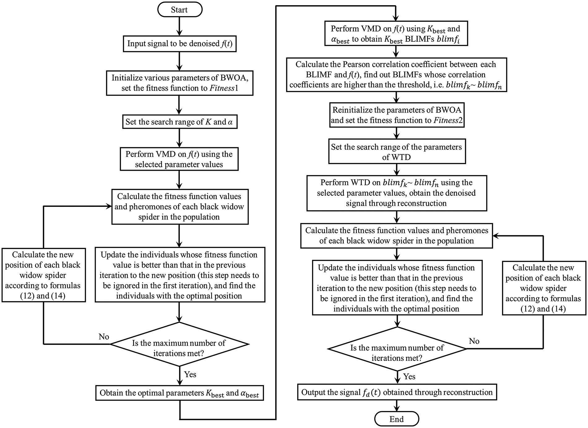
Figure 2: The denoising process of the BVW algorithm
1) Initialize various parameters of BWOA, set the search boundaries of K and
2) Perform VMD on the signal using the selected parameter values, and calculate the fitness function values and pheromones of each black widow spider in the population. The pheromone is an indicator that affects the updating of individual positions by influencing the courtship behavior of black widow spiders, which is thoroughly explained in Section 2.4.
3) Update the individuals whose fitness function value is better than that in the previous iteration to the new position (this step needs to be ignored in the first iteration), and find the individuals with the optimal position.
4) Check if the upper limit of iterations is met. If this condition is met, the optimal individual position is output as the optimal parameters, otherwise, the updated position of each black widow spider is calculated according to formulas (12) and (14), and the iterative calculation is continued by returning to steps 2) and 3).
5) Perform VMD on the signal to be denoised using the obtained optimal parameters Kbest and
6) Calculate the Pearson correlation coefficient (P-CC) between each BLIMF and the signal to be denoised, and find out the BLIMFs whose P-CCs are higher than the threshold, i.e.,
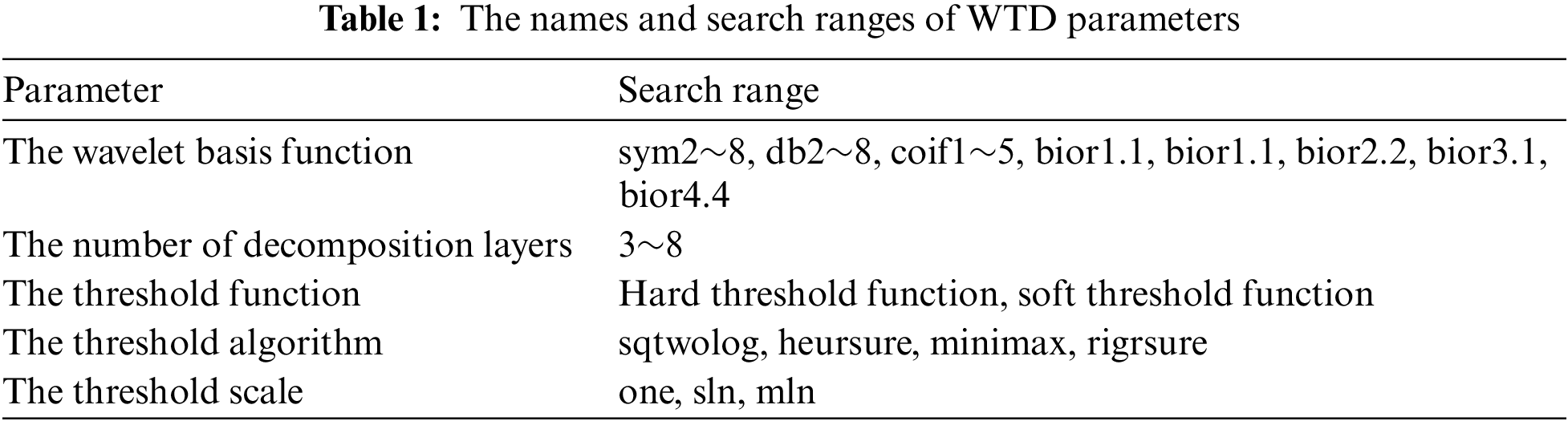
7) Reinitialize the parameters of BWOA and set the fitness function to Fitness2. The names and search ranges of WTD parameters to be selected are shown in Table 1. The search ranges are determined based on experience in the relevant researches [13,31–34].
8) Perform WTD on
9) Update the individuals whose fitness function value is better than that in the previous iteration to the new position (this step needs to be ignored in the first iteration), and find the individuals with the optimal position.
10) Check if the upper limit of iterations is met. If this condition is met, output the denoised signal obtained through reconstruction as the final result, otherwise, the updated position of each black widow spider is calculated according to formulas (12) and (14), and the iterative calculation is continued by returning to steps 8) and 9).
When searching for the effective mode functions, the P-CC threshold [35] is computed using the below equation:
where ri is P-CC between the ith BLIMF and the signal to be denoised.
2.2 Variational Mode Decomposition (VMD)
The underlying principle of VMD is to convert the problem into a variational problem and then find its solution [36]. The following is an introduction to the basic principles of VMD based on relevant research [30,37–40]. The signal undergoes VMD decomposition into various BLIMFs. To model the nonstationarity and nonlinearity of the signal, the band-limited intrinsic mode components are defined as amplitude modulation-frequency modulation harmonics [41], which may be written as
where
To assess the bandwidth of every mode, VMD is formulated as a constrained variational problem, and the constrained variational condition is [30,42]
where
Eq. (3) is a constrained variational problem. To address it and convert it into an unconstrained one, the penalty factor
The alternating direction multiplier method [45,46] is employed to alternately update
The stated formula is reformed into a nonnegative frequency interval integration to obtain the updated method of
To effectively reconstruct the signal, the update of the Lagrangian multiplier is also done with this formula:
The algorithm iterates repeatedly according to formulas (5)–(7) until meeting the convergence requirement, and the termination criterion is provided as follows:
where
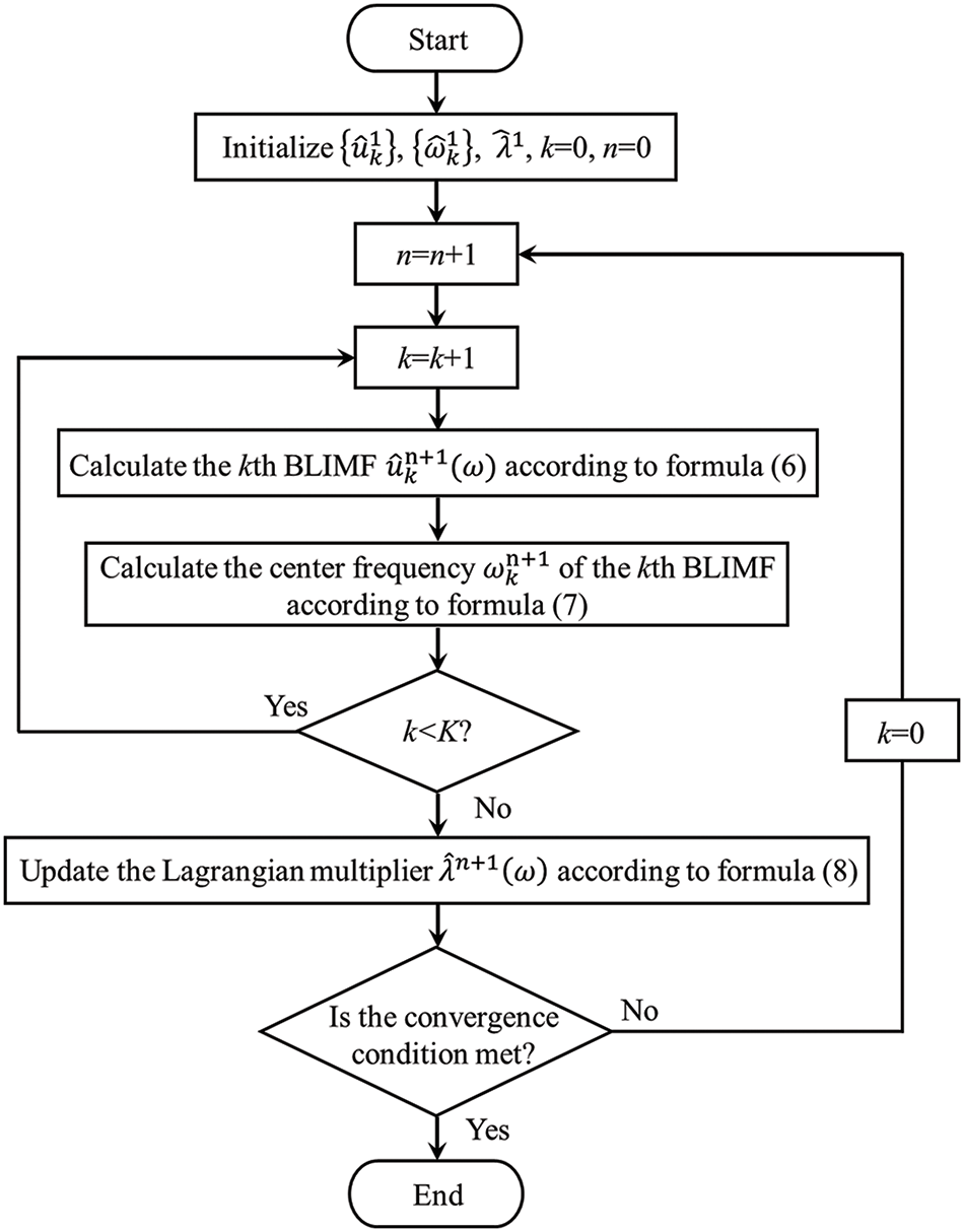
Figure 3: The implementation process of the VMD algorithm [37]
2.3 Wavelet Threshold Denoising (WTD)
WTD is a multi-scale method for signal analysis initially introduced by Donoho in 1995 [49,50], which is built upon the wavelet transform. The wavelet transform performs well in the time-frequency domain which has its foundation in the Fourier transform [51,52]. It resolves the issue where instantaneous time-domain variations are not represented in the frequency domain of the Fourier transform [53]. So WTD has found widespread application, including in electrocardiogram signal denoising [54], electromyography signal denoising [55], and image denoising [56]. In the WTD algorithm, the superposition of several wavelet basis functions of distinct scales is used to represent the signal. After wavelet decomposition, the approximation coefficients and the detail coefficients are acquired. One of their uses is to explain the association between the wavelet basis functions and the components with different frequencies. The detail coefficients correspond to the noise contained in the components with high frequencies. The detail coefficients are zeroed or shrank by a threshold function, and some approximation coefficients are retained. In this way, noise is removed from the signal.
As shown in Fig. 4, WTD consists of three main steps [57,58]: (1) Wavelet decomposition of the signal: Determine a wavelet basis function and an appropriate number of decomposition layers to decompose the signal into corresponding wavelet coefficients (including approximation coefficients and detail coefficients); (2) Wavelet coefficient threshold processing: Set an appropriate threshold for each decomposition layer, assign zero to wavelet coefficients whose absolute values fall below this threshold, and retain or shrink those with absolute values exceeding this threshold; (3) Signal reconstruction: The quantized wavelet coefficients serve to reconstruct the signal via inverse wavelet transform.
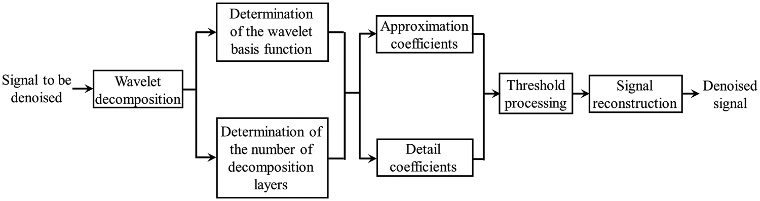
Figure 4: The schematic diagram of WTD
Fig. 5 presents the process of wavelet decomposition. In the figure, the number of decomposition layers is 3, X(t) is the signal to be denoised, and AC1 and DC1 are the approximation coefficient and detail coefficient of the first layer after X(t) decomposition, respectively. AC1 is decomposed to get the approximation coefficient AC2 and detail coefficient DC2 at the second layer, and the decomposition continues in this way until the specified number of decomposition layers is reached.
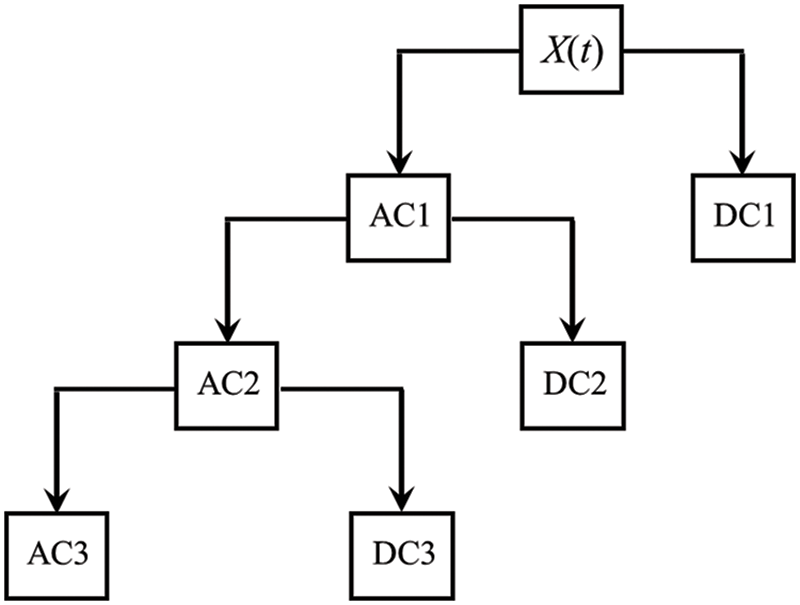
Figure 5: The schematic diagram of the wavelet decomposition
The performance of wavelet thresholding denoising is mainly affected by the wavelet basis function, the threshold algorithm, the threshold function, the threshold scale, and the number of decomposition layers [59]. When using WTD, users usually select the above parameters based on experience or trial and error, which restricts its application to a certain extent.
2.4 Black Widow Optimization Algorithm (BWOA)
BWOA is an innovative metaheuristic optimization algorithm developed in 2020 by Peña-Delgado et al. [60]. Its inspiration comes from the distinctive mating habits of black widow spiders [60]. This algorithm simulates the various movement strategies of black widow spiders during courtship and is characterized by simplicity, efficiency, quick convergence, and high precision [61]. Its inherent principle is to randomly search and gradually optimize. It requires fewer population size and iteration numbers to obtain the optimal solution, and well balances the diversification and intensification of search space [62]. So it has been applied in fields such as economic load dispatch [62], improving the precision of solar photovoltaic electrical model parameters [63], and predicting the plastic zones of underground caverns [64], and has achieved good performance. The optimization of denoising parameters for microseismic signals and the above applications are similar issues. So BWOA was adopted in this research.
In BWOA, to ensure its global search capability, a population with N individuals is initialized as
where D is the number of dimensions of the problem to be addressed. The spider’s current position (corresponding to a solution to the problem) is represented by each row of the candidate solution matrix X. Thus, the current position of the lth individual can be expressed as
where UB and LB denote the maximum and minimum limit vectors of the parameters to be searched, respectively, and rand is a random variable within the bounds of 0 and 1.
There are two ways in which a black widow spider can move on the spider web: linear and spiral. These two movements occur with different probabilities, and their mathematical model is shown below:
where Xl (t+1) and Xl (t) indicate the updated position and current position of the lth individual at the (t+1)th iteration, respectively, Xb (t) and Xr (t) represent the position of the optimal individual and a randomly chosen individual from the previous iteration (r ≠ l), respectively, m is a random value ranging from 0.4 to 0.9, while β is a random value ranging from −1 to 1.
The courtship behavior of black widow spiders is greatly influenced by pheromones. Males are able to sense high and low amounts of pheromones in the silk of females to determine how hungry they are. The pheromones from satiated females are more readily sensed by male spiders because such females have better fertility and can reduce the risk of male spiders being eaten by females. Pheromones can be expressed as follows:
where ph(l) denotes the pheromone value of the lth female spider and Fitness(l) denotes the fitness function value of the lth female spider. For the minimization problem, Fitnessmax and Fitnessmin are the poorest and best fitness function values, respectively.
Female spiders with pheromone values equal to or less than 0.3 are considered to be in a state of starvation, and it is difficult for them to mate with males. Therefore, the positions of these individuals are adjusted in accordance with the subsequent formula.
where Xr1 (t) and Xr2 (t) are the positions of two different individuals randomly chosen from the current population and σ is a randomly chosen natural number.
Setting a reasonable fitness function, i.e., the objective function, is the primary task when selecting the values of parameters using BWOA. The complexity of the time series can be reflected using the envelope entropy [65]. Following the decomposition of the signal via VMD, the BLIMF with more noise has a higher complexity and lower self-similarity in the time series [66,67], resulting in a higher envelope entropy. The BLIMF with less noise has stronger regularity, and its envelope entropy is smaller [68]. When the envelope entropy reaches the minimum value, the best decomposition performance of VMD has been achieved [69]. Therefore, we adopt the local minimum envelope entropy as the fitness function for searching for the optimal values of K and
where a(j) is the envelope signal of signal x(j) obtained after the Hilbert transformation and pj is a(j) after normalization.
where Epi is the envelope entropy of each BLIMF obtained after decomposition using VMD.
While seeking the best values of WTD parameters using BWOA, the fitness function Fitness2 is calculated using the following formula:
where SNRout is the SNR after denoising. R is P-CC between the denoised signal and the signal to be denoised. SNRout is used to filter out noise as much as possible while preserving the effective signal, while R is used to avoid results where the denoised signal has an ideal SNR but the denoised waveform is not satisfactory. The value of R ranges from −1 to 1, so no normalization is required. Considering that the SNR of the microseismic signals studied in this research is usually far less than 50, the SNRout in the above formula is normalized by dividing it by 50. 0.45 and 0.55 are weights determined based on experience, and their sum is 1.
To validate the superiority of the BVW algorithm, we first perform denoising experiments on simulated signals. A microseismic signal with weak noise is selected from microseismic signals monitored on-site, and the noise is filtered out as an original signal. The original signal is sampled at 6000 Hz. Fig. 6 presents its waveform, and the spectrum and the time-frequency representation (TFR) are presented in Fig. 7. In TFR, the time is on the x-axis and the frequency is on the y-axis, while the different colors denote the amplitude corresponding to the time and frequency. Gaussian white noise of a certain intensity was added to the original signal to synthesize the simulated signal. The SNR of the simulated signal is 8 dB, and the number of samples is 4000. Figs. 8 and 9 present the waveform, the spectrum, and the TFR of the simulated signal. As shown in Figs. 7 and 9, the frequency of the original signal is mainly in the range of 0~300 Hz. After adding white Gaussian noise, the noise frequency is distributed in the range of 0~1000 Hz.
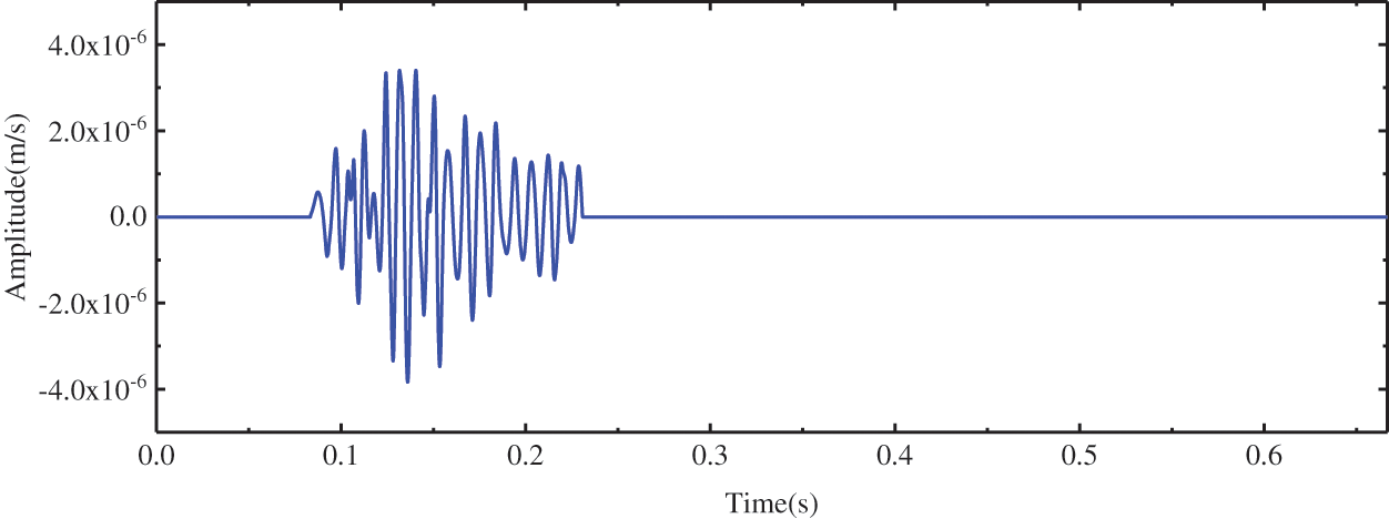
Figure 6: The waveform of the original signal
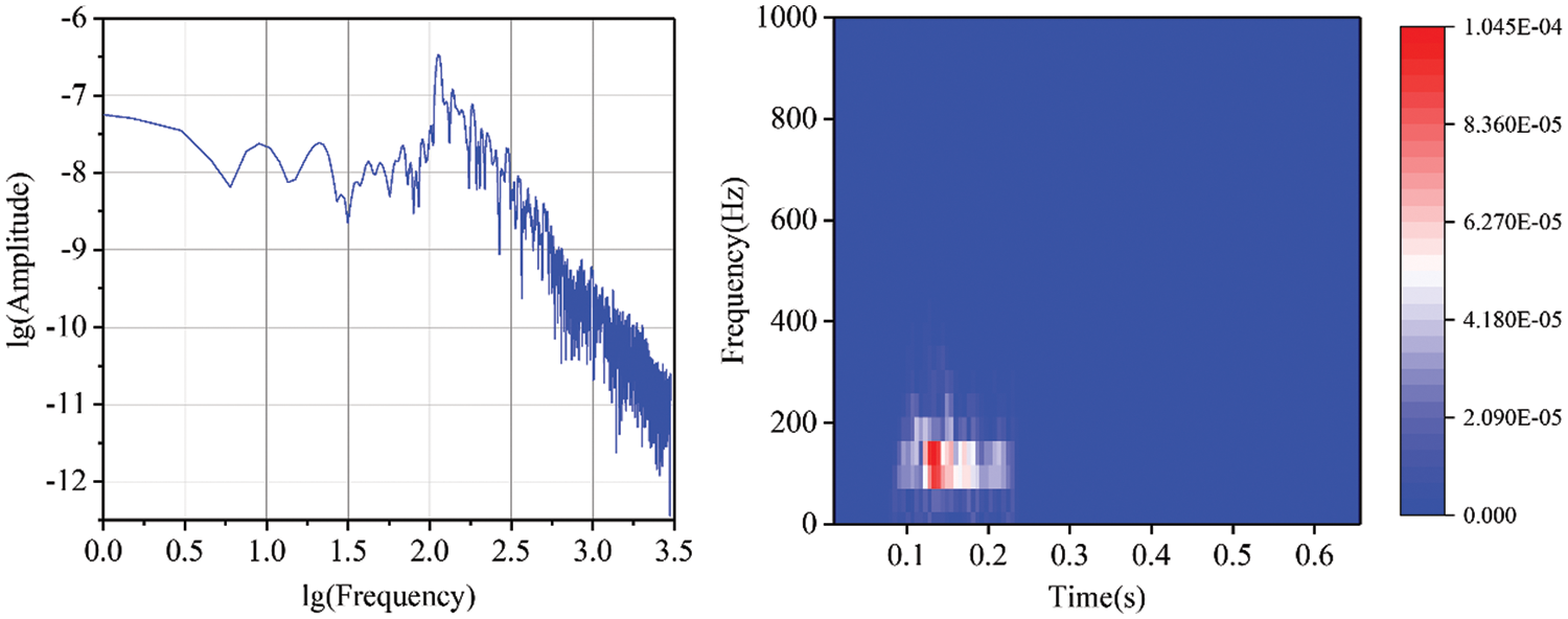
Figure 7: The spectrum and TFR of the original signal
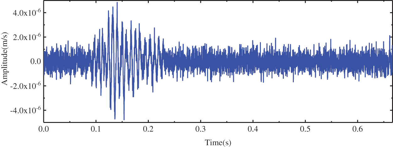
Figure 8: The waveform of the simulated signal
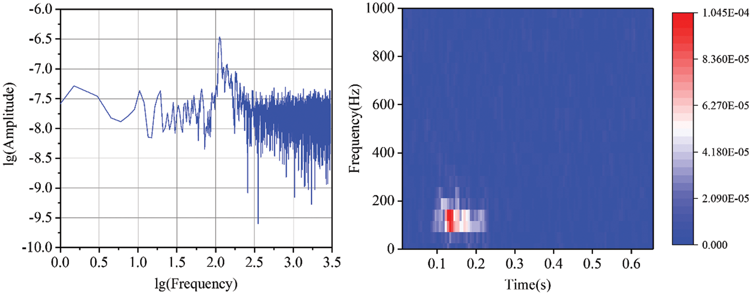
Figure 9: The spectrum and TFR of the simulated signal
To examine the denoising capability of the BVW algorithm, the VMD and EMD algorithms were introduced for comparison, and the SNR and RMSE were calculated. It should be noted that when the VMD and EMD algorithms are used for denoising, the selection rules of the mode functions used for reconstruction are the same as those of the BVW algorithm, that is, mode functions whose P-CC with the original signal exceeding the threshold are selected for reconstruction. The threshold is calculated according to formula (1).
SNR is defined as [9]
where σsingal and σnoise represent the root mean square amplitudes of the signal and the noise, respectively.
The definition of RMSE is
where s(t) is the original signal and
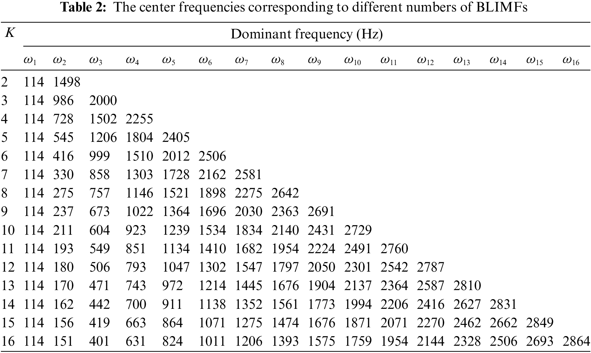
When VMD is used to denoise the simulated signal, the penalty factor
When using the BVW algorithm to denoise the simulated signal, the variations in fitness function values during the BWOA search for the best values of VMD parameters and WTD parameters are presented in Fig. 10. The best values of VMD parameters and WTD parameters were obtained at the 4th and 7th iteration, respectively, which indicates that BWOA needs only a few iterations to obtain the optimal solution, confirming the excellent performance of BWOA.
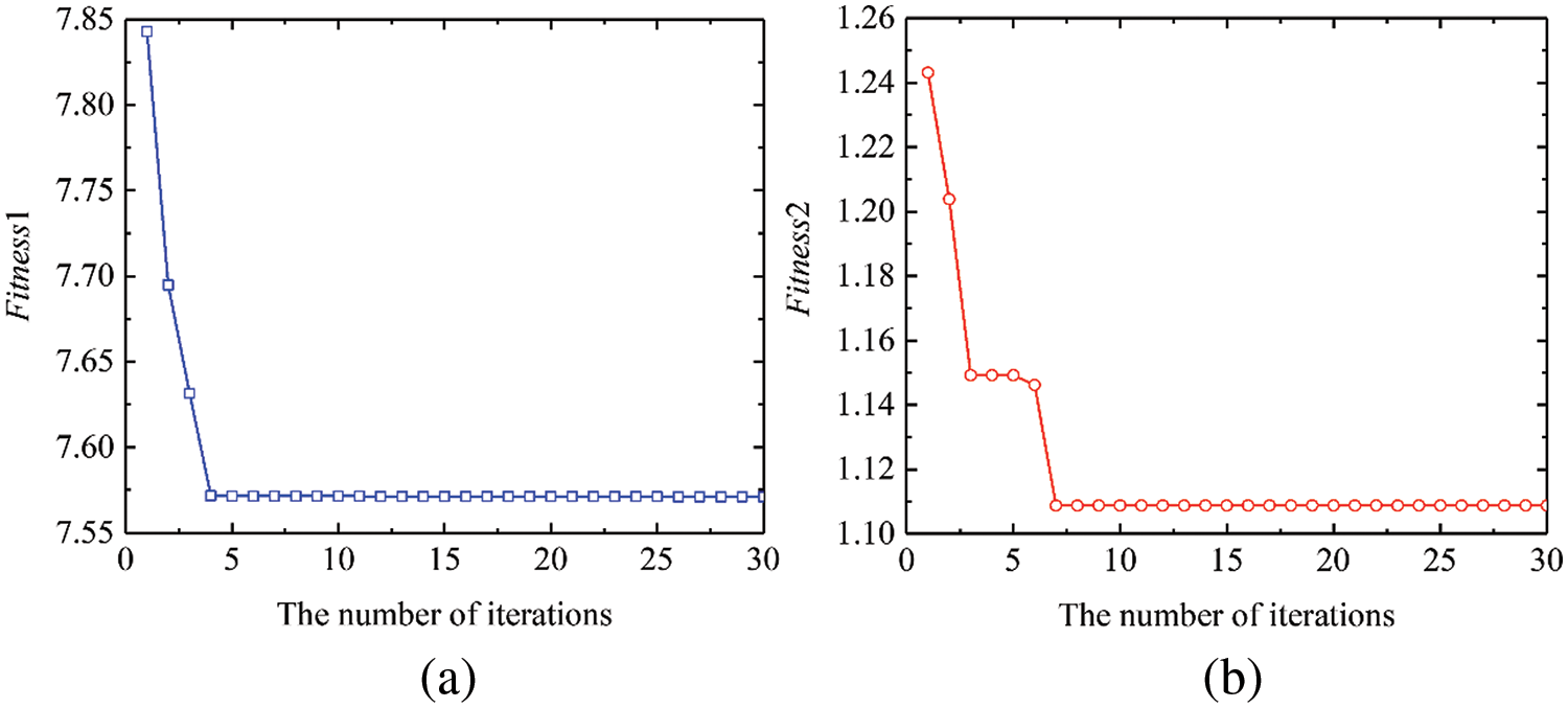
Figure 10: (a) The variation of Fitness1 value with the number of iterations in search of the best values of VMD parameters, (b) the variation of Fitness2 value with the number of iterations in search of the best values of WTD parameters
After denoising the simulated signal with the BVW, VMD, and EMD algorithms, the waveforms are presented in Fig. 11. Additionally, Fig. 12 displays the spectra and TFRs of the denoised signal. Obviously, after denoising with BVW, its waveform is the smoothest, and the attenuation of signal amplitude is reasonable, as it is the closest to the original signal. According to Fig. 11, it can be found that BVW is the most effective in filtering noise for the simulated signal, followed by VMD, with EMD being the least efficient. Fig. 12 further confirms this. Fig. 12a demonstrates that after using BVW to denoise the simulated signal, there is minimal residual noise. Meanwhile, Fig. 12b shows that after denoising using VMD, there is still residual noise with frequency ranging from 0 to 400 Hz that has not been filtered out. Additionally, Fig. 12c shows that after denoising using EMD, there is still residual noise with frequency ranging from 0 to 500 Hz that has not been filtered out.
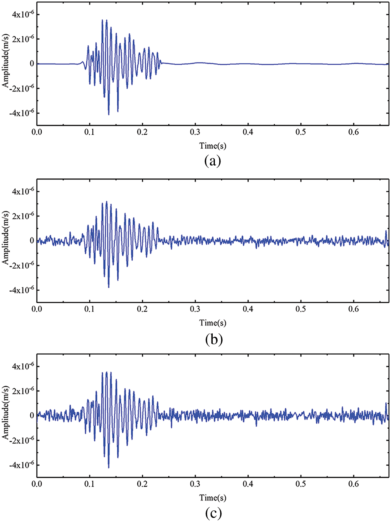
Figure 11: (a) The signal’s waveform after denoising with BVW, (b) the signal’s waveform after denoising with VMD, (c) the signal’s waveform after denoising with EMD
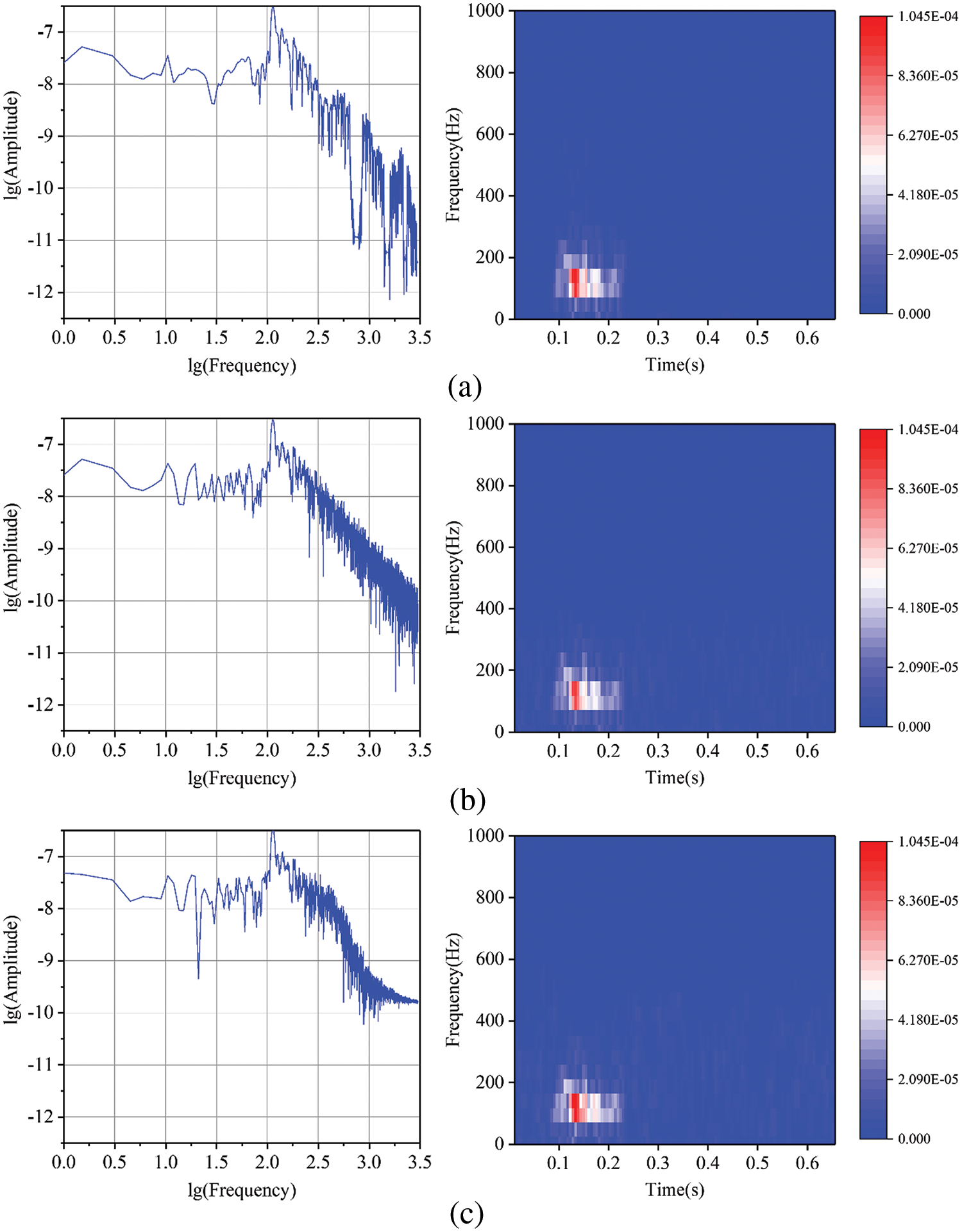
Figure 12: (a) The signal’s spectrum and TFR after denoising with BVW, (b) the signal’s spectrum and TFR after denoising with VMD, (c) the signal’s spectrum and TFR after denoising with EMD
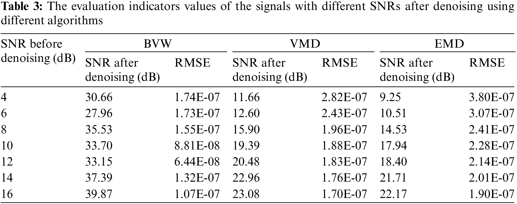
The SNR and the RMSE of the signals after denoising by the three algorithms were calculated which are displayed in Table 3. According to the table, the SNR of the simulated signal is 8 dB, the SNR increases to 14.53 dB and the RMSE is 2.41 × 10⁻⁷ after denoising using EMD. The SNR increases to 15.90 dB and the RMSE is 1.96 × 10⁻⁷ after denoising using VMD. After denoising using BVW, the SNR increased to 35.53 dB and the RMSE was 1.55 × 10⁻⁷. The evaluation indicators values after denoising using BVW are the most excellent.
In summary, BVW benefits from better values of VMD parameters and WTD parameters, which can further filter low- and intermediate-frequency noise in the signal. In addition, the waveform after denoising using BVW is closer to the original signal, its SNR is higher, and its RMSE is lower. Therefore, BVW achieved the best denoising performance.
To further illustrate the effectiveness of the BVW algorithm, simulated signals with different SNRs were synthesized by adding Gaussian white noise with different intensities to the above original signal, which means that only the Gaussian noise magnitude was changed without changing the original signal. The previously mentioned three algorithms were utilized to denoise the above-simulated signals and the SNR and RMSE after denoising are calculated, as displayed in Table 3 and Fig. 13. The BVW algorithm can obtain a higher SNR and a lower RMSE under the noise of different intensities, and the denoising performance is greatly superior to that of VMD and EMD.
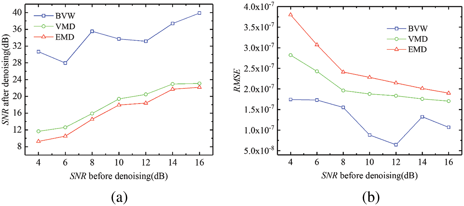
Figure 13: The evaluation indicators values of the signals with various SNRs after denoising through various algorithms
To validate the applicability of the BVW algorithm to microseismic signals monitored on-site, microseismic signals from Fankou Lead-Zinc Mine were denoised. As shown in Fig. 14, the position of Fankou Lead-Zinc Mine is in Shaoguan City, South China. The mine is an underground metal mine famous for using the vertical crater retreat mining method to extract ore, and the minimum mining level is more than 850 m from the surface. To prevent ground pressure disasters, Fankou Lead-Zinc Mine installed the microseismic monitoring system from the Institute of Mine Seismology at the end of 2016. As shown in Fig. 15, the system consists of 26 uniaxial geophones and 6 triaxial geophones, which are installed at 5 different levels [2].
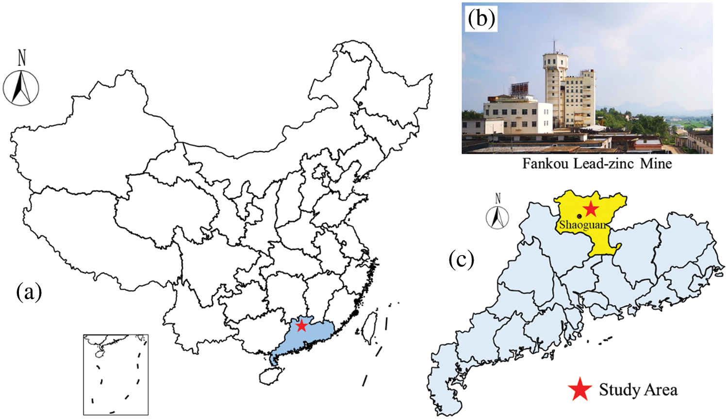
Figure 14: The schematic diagrams of mine location: (a) The location of Fankou Lead-Zinc Mine in China, (b) the main shaft of the mine, (c) the location of the mine in Guangdong province
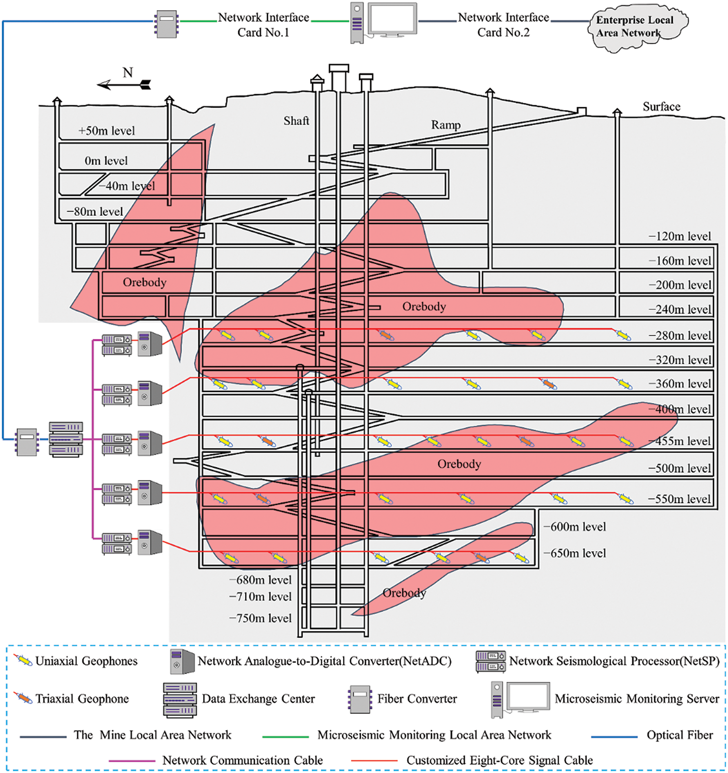
Figure 15: The development system and microseismic monitoring system of the mine
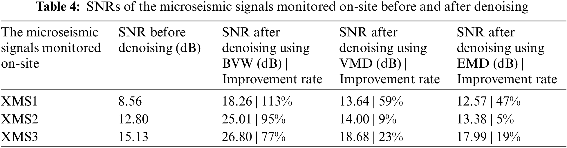
Three relatively typical microseismic signals (XMS1, XMS2, and XMS3) with different intensities of noise were selected randomly from microseismic signals monitored on-site to verify the universality of the algorithm. The sampling frequencies of the microseismic signals monitored on site are 6000 Hz, and their SNRs are 8.56, 12.80, and 15.13 dB, respectively. The numbers of samples are 3500, 2500, and 6000, respectively. These three signals were denoised using the BVW, VMD, and EMD algorithms.
The waveforms of XMS1 pre- and post-denoising are presented in Fig. 16. Additionally, Fig. 17 displays the spectra and TFRs of XMS1 pre- and post-denoising. Fig. 17a demonstrates that the frequency of the noise is primarily in the range of 0~200 Hz, and there is also distribution in 300~500 Hz and 700~800 Hz. Fig. 17b indicates that the denoising with BVW is more efficient with less residual noise. Conversely, after denoising with VMD, Fig. 17c still exhibits residual noise within the ranges of 100~200 Hz and 400~500 Hz. Similarly, after denoising with EMD, Fig. 17d also presents residual noise within the ranges of 400~500 Hz and 700~800 Hz.
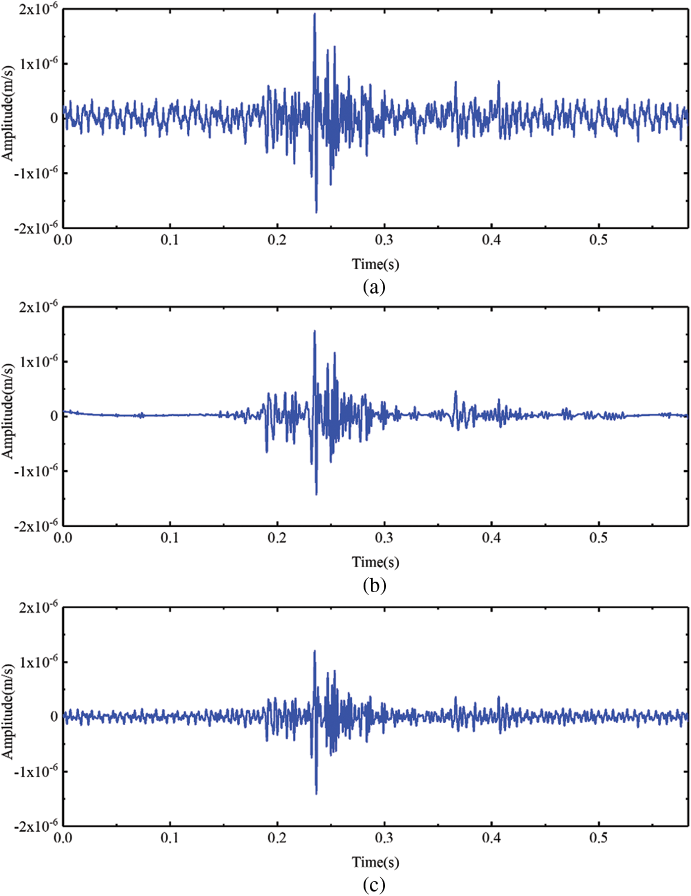
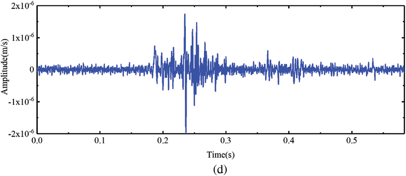
Figure 16: (a) The waveform of XMS1, (b) the waveform of the signal after XMS1 denoised using the BVW algorithm, (c) the waveform of the signal after XMS1 denoised using the VMD algorithm, (d) the waveform of the signal after XMS1 denoised using the EMD algorithm
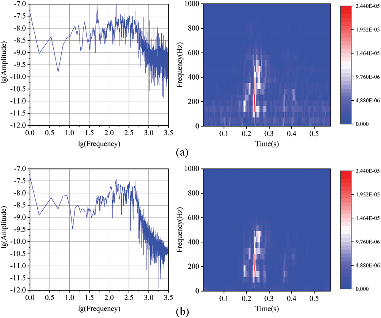
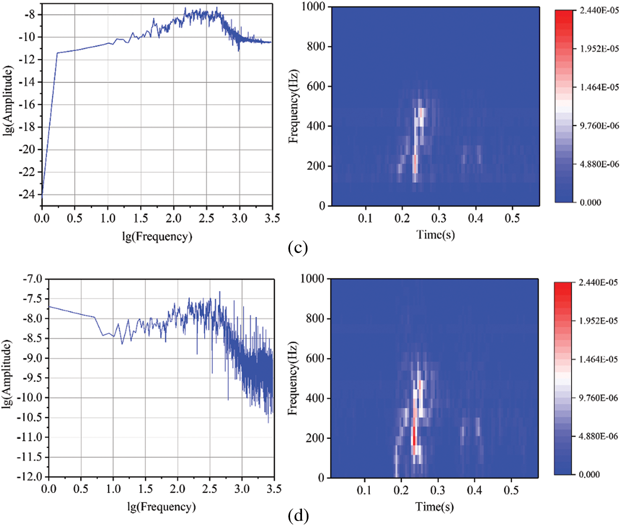
Figure 17: (a) The spectrum and TFR of XMS1, (b) the spectrum and TFR of the signal after XMS1 denoised using the BVW algorithm, (c) the spectrum and TFR of the signal after XMS1 denoised using the VMD algorithm, (d) the spectrum and TFR of the signal after XMS1 denoised using the EMD algorithm
The waveforms of XMS2 pre- and post-denoising are presented in Fig. 18. Additionally, Fig. 19 displays the spectra and TFRs of XMS2 before and after denoising. Fig. 19a reflects that the noise frequency is primarily within the 0~500 Hz range. After denoising with BVW, there is very little residual noise, which can be seen in Fig. 19b. Conversely, after denoising with VMD, Fig. 19c still exhibits residual noise within the ranges of 100~300 Hz. Similarly, after denoising with EMD, Fig. 19d also presents residual noise within the ranges of 300~500 Hz. So the denoising with BVW is more efficient.
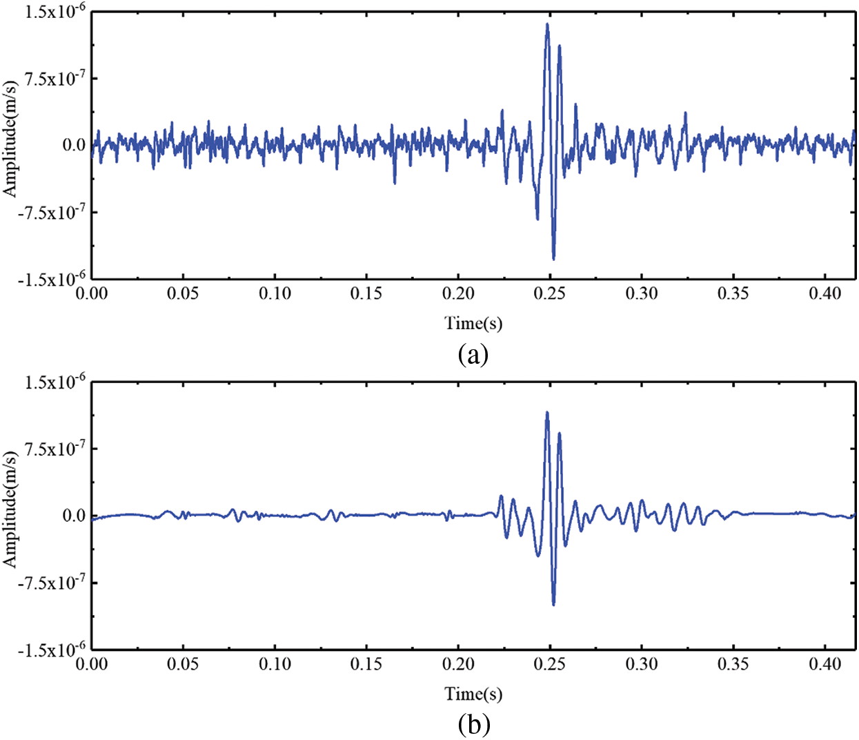
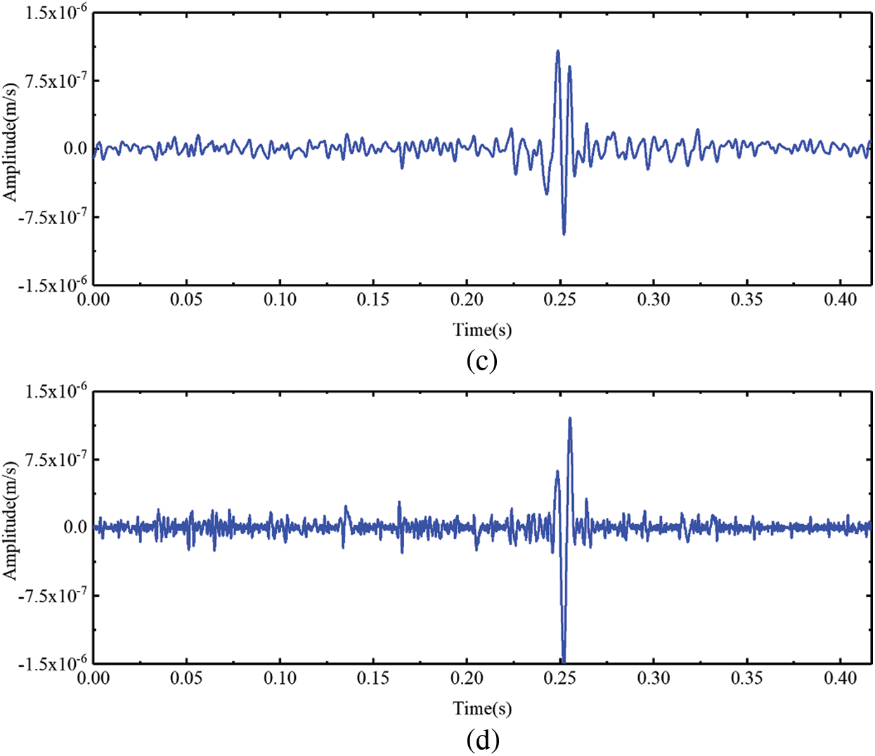
Figure 18: (a) The waveform of XMS2, (b) the waveform of the signal after XMS2 denoised using the BVW algorithm, (c) the waveform of the signal after XMS2 denoised using the VMD algorithm, (d) the waveform of the signal after XMS2 denoised using the EMD algorithm
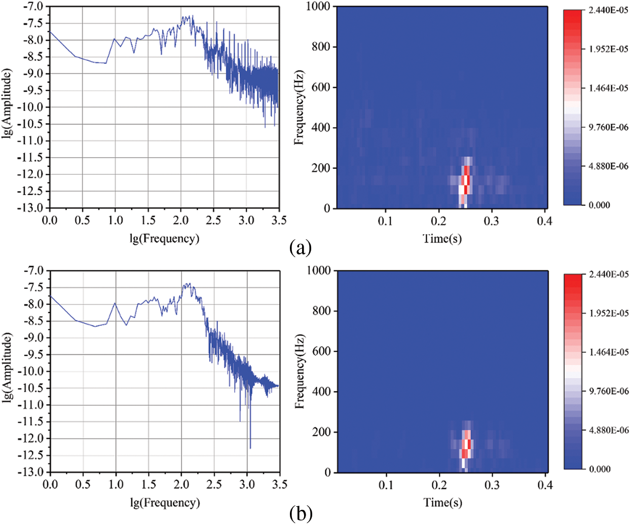
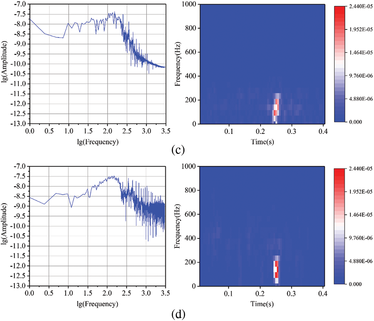
Figure 19: (a) The spectrum and TFR of XMS2, (b) the spectrum and TFR of the signal after XMS2 denoised using the BVW algorithm, (c) the spectrum and TFR of the signal after XMS2 denoised using the VMD algorithm, (d) the spectrum and TFR of the signal after XMS2 denoised using the EMD algorithm
The waveforms of XMS3 pre- the noise is primarily inand post-denoising are presented in Fig. 20. Additionally, Fig. 21 displays the spectra and TFRs of XMS3 pre- and post-denoising. Fig. 21a demonstrates that the noise frequency is primarily within the 0~500 Hz range. After denoising with BVW, there is very little residual noise, which can be seen in Fig. 21b. However, after using VMD for denoising, there is a large amount of residual noise with frequencies ranging from 0~300 Hz, which can be seen in Fig. 21c. Similarly, after denoising with EMD, Fig. 21d also presents residual noise within the ranges of 100~400 Hz. Obviously, the denoising with BVW is more efficient.
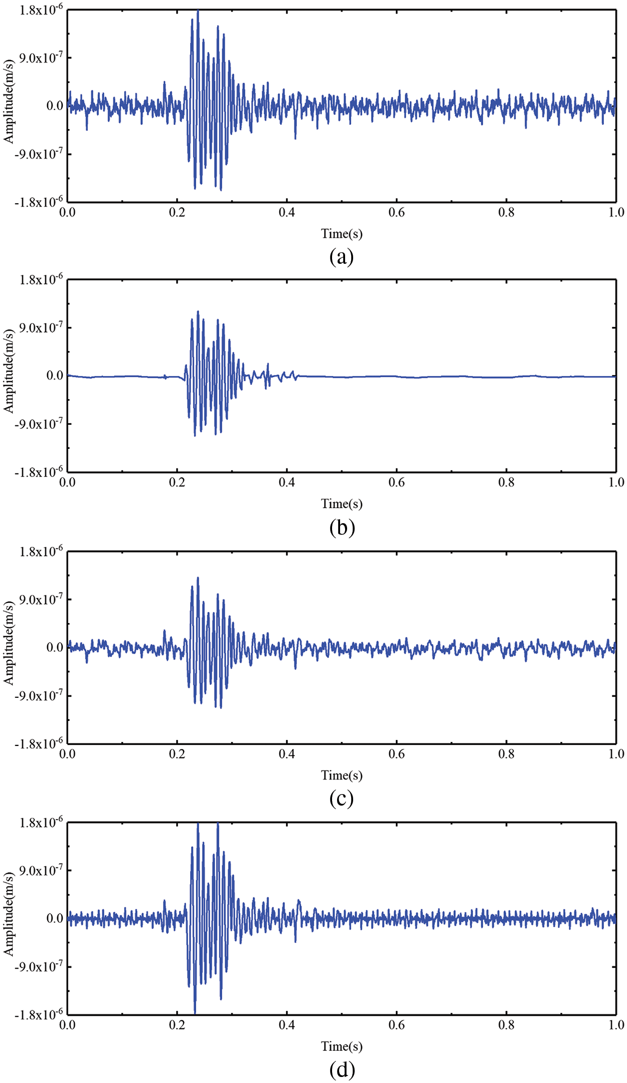
Figure 20: (a) The waveform of XMS3, (b) the waveform of the signal after XMS3 denoised using the BVW algorithm, (c) the waveform of the signal after XMS3 denoised using the VMD algorithm, (d) the waveform of the signal after XMS3 denoised using the EMD algorithm
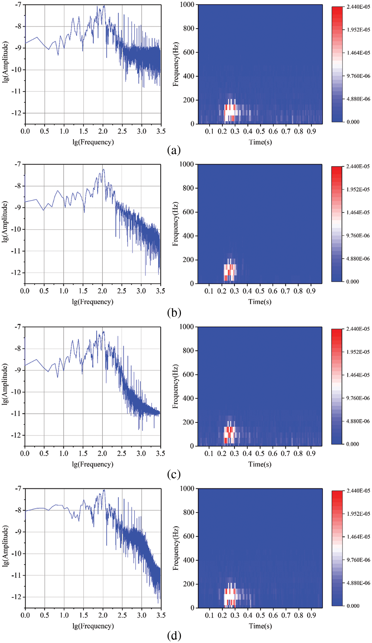
Figure 21: (a) The spectrum and TFR of XMS3, (b) the spectrum and TFR of the signal after XMS3 denoised using the BVW algorithm, (c) the spectrum and TFR of the signal after XMS3 denoised using the VMD algorithm, (d) the spectrum and TFR of the signal after XMS3 denoised using the EMD algorithm
The SNRs of XMS1, XMS2, and XMS3 before and after denoising were calculated and shown in Table 4. The improvement rates of the SNRs after denoising compared to the SNRs before denoising have also been calculated and presented. The table shows that after denoising with BVW, VMD, and EMD, the SNR has been improved, but the improvement with BVW denoising is more significant because its improvement rate is the largest. This also confirms the conclusion that the denoising with BVW is more efficient.
The BVW algorithm presented in this research integrates the VMD algorithm, thereby avoiding the issues with mode mixing and the deficiency of a solid mathematical theoretical foundation commonly found in EMD and its improved methods. Additionally, the BVW algorithm utilizes BWOA to find the best VMD parameter values, resulting in superior decomposition performance and enhanced usability of VMD. Furthermore, in the BVW algorithm, the best values of WTD parameters are acquired through searching with BWOA. That solved the problem of relying on experience for parameter value selection and requiring a large workload in the application of the WTD algorithm, which greatly improved the usability and efficiency of WTD.
However, there are some limitations to the algorithm. When using the BVW algorithm to denoise common microseismic signals in mines on a laptop computer equipped with an Intel Core i78500U CPU, the time consumed is less than 3 min. But for more complex signals, it may require a workstation with stronger computing power to complete the denoising quickly. In addition, when BWOA is used for optimization to obtain the best values of WTD parameters, the weights in the fitness function formula, i.e., 0.45 and 0.55, are determined based on experience, potentially limiting the applicability of the algorithm. The authors intend to address these issues in their subsequent research.
A new algorithm called BVW is presented for denoising microseismic signals in this research. The BVW algorithm utilizes VMD to decompose microseismic signals and then uses WTD to filter out the residual low- and intermediate-frequency noise in the effective mode functions. Finally, the denoised microseismic signal is acquired through reconstruction. The values of VMD parameters (the number of BLIMFs K and penalty factor
Acknowledgement: The authors wish to express sincere appreciation to the reviewers for their valuable comments that enhanced the paper’s quality. We also sincerely appreciate the editors for their patience, supportive reminders, and dedicated efforts in editing the manuscript.
Funding Statement: This research is funded by the National Natural Science Foundation of China (Grant No. 51874350), the National Natural Science Foundation of China (Grant No. 52304127), the Fundamental Research Funds for the Central Universities of Central South University (Grant No. 2020zzts200), the Science Foundation of the Fuzhou University (Grant No. 511229) and Fuzhou University Testing Fund of Precious Apparatus (Grant No. 2024T040).
Author Contributions: The authors confirm contribution to the paper as follows: study conception and design: Dijun Rao, Zhengxiang He; data collection: Min Huang, Xiuzhi Shi; analysis and interpretation of results: Dijun Rao, Zhi Yu; draft manuscript preparation: Dijun Rao, Min Huang. All authors reviewed the results and approved the final version of the manuscript.
Availability of Data and Materials: The data that support the findings of this study are available from the first and corresponding authors upon reasonable request.
Conflicts of Interest: Dijun Rao and Min Huang were employed by the Zijin Mining Group Co., Ltd., and Zijin (Changsha) Engineering Technology Co., Ltd. The authors declare that they have no conflicts of interest to report regarding the present study.
References
1. Zhang JY, Jiang RC, Li B, Xu NW. An automatic recognition method of microseismic signals based on EEMD-SVD and ELM. Comput Geosci. 2019;133:104318. doi:10.1016/j.cageo.2019.104318. [Google Scholar] [CrossRef]
2. Rao DJ, Shi XZ, Zhou J, Yu Z, Gou YG, Dong ZZ, et al. An expert artificial intelligence model for discriminating microseismic events and mine blasts. Appl Sci. 2021;11(14):6474. doi:10.3390/app11146474. [Google Scholar] [CrossRef]
3. Brown L, Hudyma M. Identification of stress change within a rock mass through apparent stress of local seismic events. Rock Mech Rock Eng. 2017;50:81–8. doi:10.1007/s00603-016-1092-z. [Google Scholar] [CrossRef]
4. He ZX, Xu XL, Rao DJ, Peng PA, Wang JH, Tian SC. PSSegNet: segmenting the P- and S-phases in microseismic signals through deep learning. Mathematics. 2024;12(1):130. doi:10.3390/math12010130. [Google Scholar] [CrossRef]
5. Palo M, Ogliari E, Sakwa M. Spatial pattern of the seismicity induced by geothermal operations at the geysers (California) inferred by unsupervised machine learning. IEEE Trans Geosci Remote Sens. 2024;62:1–13. doi:10.1109/TGRS.2024.3361169. [Google Scholar] [CrossRef]
6. Palo M, Picozzi M, de Landro G, Zollo A. Microseismicity clustering and mechanic properties reveal fault segmentation in southern Italy. Tectonophysics. 2023;856:229849. doi:10.1016/j.tecto.2023.229849. [Google Scholar] [CrossRef]
7. Xiao YX, Feng XT, Hudson JA, Chen BR, Feng GL, Liu JP. ISRM suggested method for in situ microseismic monitoring of the fracturing process in rock masses. Rock Mech Rock Eng. 2016;49:343–69. doi:10.1007/s00603-015-0859-y. [Google Scholar] [CrossRef]
8. Zhang XL, Lu XM, Jia RS, Kan ST. Micro-seismic signal denoising method based on variational mode decomposition and energy entropy. J China Coal Soc. 2018;43(2):356–63 (In Chinese). doi:10.13225/j.cnki.jccs.2017.4153. [Google Scholar] [CrossRef]
9. Huang WX, Liu DW. Mine microseismic signal denosing based on variational mode decomposition and independent component analysis. J Vib Shock. 2019;38(4):56–63. doi:10.1007/s00024-023-03365-0. [Google Scholar] [CrossRef]
10. Mallat SG. A theory for multiresolution signal decomposition: the wavelet representation. IEEE Trans Pattern Anal Mach Intell. 1989;11(7):674–93. doi:10.1109/34.192463. [Google Scholar] [CrossRef]
11. Huang NE, Shen Z, Long SR. A new view of nonlinear water waves: the Hilbert spectrum. Annu Rev Fluid Mech. 1999;31:417–57. doi:10.1146/annurev.fluid.31.1.417. [Google Scholar] [CrossRef]
12. Wu ZH, Huang NE. Ensemble empirical mode decomposition: a noise-assisted data analysis method. Adv Adapt Data Anal. 2009;1(1):1–41. doi:10.1142/S1793536909000047. [Google Scholar] [CrossRef]
13. Xu HB, Li SL, Chen JJ. A study on method of signal denoising based on wavelet transform for micro-seismicity monitoring in large-scale rockmass structures. Acta Seismol Sin. 2012;34(1):85–96. doi:10.3969/j.issn.0253-3782.2012.01.008. [Google Scholar] [CrossRef]
14. Valencia D, Orejuela D, Salazar J, Valencia J. Comparison analysis between rigrsure, sqtwolog, heursure and minimaxi techniques using hard and soft thresholding methods. In: 2016 XXI Symposium on Signal Processing, Images and Artificial Vision (STSIVA); Bucaramanga, Colombia; 2016. p. 1–5. doi:10.1109/STSIVA.2016.7743309. [Google Scholar] [CrossRef]
15. Chen DY, Cao CX, Peng W. Method of time-frequency analysis of engineering signals using wavelet. J Chongqing Univ. 1999;22(5):27–31 (In Chinese). [Google Scholar]
16. Su MZ. Risk zone identification of slope based on microseismic monitoring. Xi’an University of Architecture and Technology:China; 2021. doi:10.15244/pjoes/187142. [Google Scholar] [CrossRef]
17. Huang NE, Shen Z, Long SR, Wu MC, Shi HH, Yen N, et al. The empirical mode decomposition and the Hilbert spectrum for nonlinear and non-stationary time series analysis. Proc R Soc A. 1998;454(1971):903–95. doi:10.1098/rspa.1998.0193. [Google Scholar] [CrossRef]
18. Liang Z, Peng SP, Zheng J. Self-adaptive denoising for microseismic signal based on EMD and mutual information entropy. Comput Eng Appl. 2014;50(4):7–11. [Google Scholar]
19. Li X, Dong LL, Li B, Lei YF, Xu NW. Microseismic signal denoising via empirical mode decomposition, compressed sensing, and soft-thresholding. Appl Sci. 2020;10(6):2191. doi:10.3390/app10062191. [Google Scholar] [CrossRef]
20. Liu SX, Chen YH, Luo CP, Jiang HJ, Li H, Li HQ, et al. Particle swarm optimization-based variational mode decomposition for ground penetrating radar data denoising. Remote Sens. 2022;14(13):2973. doi:10.3390/rs14132973. [Google Scholar] [CrossRef]
21. Tang BP, Dong SJ, Song T. Method for eliminating mode mixing of empirical mode decomposition based on the revised blind source separation. Signal Process. 2012;92(1):248–58. doi:10.1016/j.sigpro.2011.07.013. [Google Scholar] [CrossRef]
22. Li W, Jiang XL, Chen HB, Jin ZP, Liu ZJ, Li XW, et al. Denosing method of mine microseismic signal based on EEMD_Hankel_SVD. J China Coal Soc. 2018;43(7):1910–7 (In Chinese). doi:10.1007/s11227-022-04554-9. [Google Scholar] [CrossRef]
23. Su MZ, Li FB, Lu CW, Zhang S, He YG. Noise reduction of microseismic signal based on VMD-SSA. Prog Geophys. 2020;1–13. [Google Scholar]
24. Dong LL, Jiang RC, Xu NW, Qian B. Research on microseismic signal denoising method based on LMD-SVD. Adv Eng Sci. 2019;50(5):126–36. [Google Scholar]
25. Li J, Li Y, Li Y, Qian ZH. Downhole microseismic signal denoising via empirical wavelet transform and adaptive thresholding. J Geophys Eng. 2018;15(6):2469–80. doi:10.1088/1742-2140/aacf63. [Google Scholar] [CrossRef]
26. Peng PA, Wang LG. A nonparametric method for automatic denoising of microseismic data. Shock Vib. 2018;2018:1–8. doi:10.1155/2018/4367201. [Google Scholar] [CrossRef]
27. Dragomiretskiy K, Zosso D. Variational mode decomposition. IEEE Trans Signal Process. 2014;62(3):531–44. doi:10.1109/TSP.2013.2288675. [Google Scholar] [CrossRef]
28. Zhou Y, Li L, Wang K, Zhang X, Gao C. Coherent doppler wind lidar signal denoising adopting variational mode decomposition based on honey badger algorithm. Opt Express. 2022;30(14):25774–87. doi:10.1364/OE.461116. [Google Scholar] [PubMed] [CrossRef]
29. Liu X, Wang Z, Li M, Yue C, Liang SY, Wang L. Feature extraction of milling chatter based on optimized variational mode decomposition and multi-scale permutation entropy. Int J Adv Manuf Technol. 2021;114(9–10):2849–62. doi:10.1007/s00170-021-07027-0. [Google Scholar] [CrossRef]
30. Li H, Chang J, Xu F, Liu Z, Yang Z, Zhang L, et al. Efficient lidar signal denoising algorithm using variational mode decomposition combined with a whale optimization algorithm. Remote Sens. 2019;11(2):126. doi:10.3390/rs11020126. [Google Scholar] [CrossRef]
31. Chen Z, Ding LL, Luo H, Song BY, Zhang M, Pan YS. Mine microseismic events classification based on improved wavelet decomposition and ELM. J China Coal Soc. 2020;45(S2):637–48 (In Chinese). doi:10.1007/s12559-022-09997-z. [Google Scholar] [CrossRef]
32. Zhu XH, Chen BR, Li T, Wei FB, Wang X. FIR-wavelet joint filtering algorithm for microseismic signals and its application. Chinese J Rock Mech Eng. 2020;9:1872–82 (In Chinese). [Google Scholar]
33. Gong Y, Jia RS, Lu XM, Peng YJ, Zhao WD, Zhang XL. To suppress the random noise in microseismic signal by using empirical mode decomposition and wavelet transform. J China Coal Soc. 2018;11:3247–56 (In Chinese). doi:10.13225/j.cnki.jccs.2017.1667. [Google Scholar] [CrossRef]
34. Tang LZ, Chen ZN, Zhang J, Gao LH. Research and analysis on wavelet of mine microseismic signals. Sci Technol Rev. 2013;31(32):29–33. [Google Scholar]
35. Du Y, Li H, Liu QQ, Lu JY, Li F. Research on improved method for denoising of PSO-VMD-SVD. J Jilin Univ (Information Sci Ed). 2021;39(2):142–51 (In Chinese). [Google Scholar]
36. Zhao DM, Du G, Liu X, Wu ZQ, Li C. Wind power combination prediction model based on time series decomposition and machine learning. Mod Electr Power. 2022;39(1):9–18. [Google Scholar]
37. Long J, Wang X, Dai D, Tian M, Zhu G, Zhang J. Denoising of UHF PD signals based on optimised VMD and wavelet transform. IET Sci Meas Technol. 2017;11(6):753–60. doi:10.1049/iet-smt.2016.0510. [Google Scholar] [CrossRef]
38. Wang X, Pang X, Wang Y. Optimized VMD-wavelet packet threshold denoising based on cross-correlation analysis. Int J Performability Eng. 2018;14(9):2239–47. doi:10.23940/ijpe.18.09.p33.22392247. [Google Scholar] [CrossRef]
39. Zhang J, He J, Long J, Yao M, Zhou W. A new denoising method for UHF PD signals using adaptive VMD and SSA-based shrinkage method. Sensors. 2019;19(7):1594. doi:10.3390/s19071594. [Google Scholar] [PubMed] [CrossRef]
40. Lei Y, Liu L, Bai WL, Feng HX, Wang ZY. Seismic signal analysis based on adaptive variational mode decomposition for high-speed rail seismic waves. Appl Geophys. 2023;21:358–71. doi:10.1007/s11770-023-1034-y. [Google Scholar] [CrossRef]
41. Ding MK, Shi ZY, Du BH, Wang HG, Han LY. A signal de-noising method for a MEMS gyroscope based on improved VMD-WTD. Meas Sci Technol. 2021;32(9):95112. doi:10.1088/1361-6501/abfe33. [Google Scholar] [CrossRef]
42. Wang P, Gao Y, Wu M, Zhang F, Li G, Qin C. A denoising method for fiber optic gyroscope based on variational mode decomposition and beetle swarm antenna search algorithm. Entropy. 2020;22(7):765. doi:10.3390/e22070765. [Google Scholar] [PubMed] [CrossRef]
43. Zhao S, Zhou YL, Shu XW. Compensation of fiber optic gyroscope vibration error based on VMD and FPA-WT. Meas Sci Technol. 2022;33(11):115104. doi:10.1088/1361-6501/ac7849. [Google Scholar] [CrossRef]
44. Wang Q, Hu S, Wang XY. Detection of incipient rotor unbalance fault based on the RIME-VMD and modified-WKN. Sci Rep. 2024;14(1):1–15. doi:10.1038/s41598-024-54984-z. [Google Scholar] [PubMed] [CrossRef]
45. Li Y, Li Y, Chen X, Yu J. Denoising and feature extraction algorithms using NPE combined with VMD and their applications in ship-radiated noise. Symmetry. 2017;9(11):256. doi:10.3390/sym9110256. [Google Scholar] [CrossRef]
46. Zhou ZY, Ding S, Zhu K. Reducing the noise in power quality disturbance with VMD. In: 2022 IEEE 2nd International Conference on Power, Electronics and Computer Applications (ICPECA); 2022; Shenyang, China, IEEE. p. 52–6. [Google Scholar]
47. Ma P, Zhang HL, Fan WH, Wang C. Early fault detection of bearings based on adaptive variational mode decomposition and local tangent space alignment. Eng Comput. 2019;36(2):509–32. doi:10.1108/EC-05-2018-0206. [Google Scholar] [CrossRef]
48. Hu HP, Zhang LM, Yan HC, Bai YP, Wang P. Denoising and baseline drift removal method of MEMS hydrophone signal based on VMD and wavelet threshold processing. IEEE Access. 2019;7:59913–22. doi:10.1109/ACCESS.2019.2915612. [Google Scholar] [CrossRef]
49. Donoho DL. De-noising by soft-thresholding. IEEE Trans Inf Theory. 1995;41(3):613–27. doi:10.1109/18.382009. [Google Scholar] [CrossRef]
50. Wang Z, Liu Y, Du J, Wang Z, Shao Q. De-noising magnetotelluric data using variational mode decomposition combined with mathematical morphology filtering and wavelet thresholding. J Appl Geophys. 2022;204:104751. doi:10.1016/j.jappgeo.2022.104751. [Google Scholar] [CrossRef]
51. Cui HM, Zhao RM, Hou YL. Improved threshold denoising method based on wavelet transform. Phys Procedia. 2012;33:1354–9. doi:10.1016/j.phpro.2012.05.222. [Google Scholar] [CrossRef]
52. Wang ZZ, Ding HB, Wang BX, Liu D. New denoising method for lidar signal by the WT-VMD joint algorithm. Sensors. 2022;22(16):5978. doi:10.3390/s22165978. [Google Scholar] [PubMed] [CrossRef]
53. Liu M, Wang EY, Liu ZT, Xu FL, Zhang Y, Yu XY. Application of wavelet denoising in processing the micro-seismic signal of coal-rock. Min Res Dev. 2011;31(2):67–70. doi:10.3390/app14041509. [Google Scholar] [CrossRef]
54. Karthikeyan P, Murugappan M, Yaacob S. ECG signal denoising using wavelet thresholding techniques in human stress assessment. Int J Electr Eng Inform. 2012;4(2):306. doi:10.15676/ijeei.2012.4.2.9. [Google Scholar] [CrossRef]
55. Phinyomark A, Limsakul C, Phukpattaranont P. An optimal wavelet function based on wavelet denoising for multifunction myoelectric control. In: 2009 6th International Conference on Electrical Engineering/Electronics, Computer, Telecommunications and Information Technology; 2009; Chonburi, Thailand, IEEE. vol. 2, p. 1098–101. doi:10.1109/ECTICON.2009.5137236. [Google Scholar] [CrossRef]
56. Kaur L, Gupta S, Chauhan RC. Image denoising using wavelet thresholding. In: Proceedings of the Third Indian Conference on Computer Vision, Graphics & Image Processing (ICVGIP); 2002; Ahmadabad, India. vol. 2, p. 16–8. [Google Scholar]
57. Zhou X, Wang X, Yang Y, Guo J, Wang P. De-noising of high-speed turnout vibration signals based on wavelet threshold. J Vib Shock. 2014;33(23):200–6 (In Chinese). [Google Scholar]
58. Wang Z, Zhu NN, Zheng X. Research on partial discharge pattern recognition method of switchgear based on LDA and RBF neural network. Electron Meas Technol. 2021;44(14):148–52. doi:10.1088/1742-6596/1659/1/012057. [Google Scholar] [CrossRef]
59. Wang QQ. Research on analytical method and function construction method of aircraft telemetry data. Xi’an Technological University: Xi’an, China; 2019. [Google Scholar]
60. Peña-Delgado AF, Peraza-Vázquez H, Almazán-Covarrubias JH, Torres Cruz N, García-Vite PM, Morales-Cepeda AB, et al. A novel bio-inspired algorithm applied to selective harmonic elimination in a three-phase eleven-level inverter. Math Probl Eng. 2020;2020:1–10. doi:10.1155/2020/8856040. [Google Scholar] [CrossRef]
61. Fu YM, Xu LQ, Qi KH, Shen YM, Qu CW. Multi-objective black widow algorithm guided by competitive mechanism and pheromone mechanism. J Front Comput Sci Technol. 2023;17(12):2913–27 (In Chinese). [Google Scholar]
62. Pawani K, Singh M. Economic load dispatch using black widow optimization algorithm. In: 2021 IEEE 2nd International Conference on Electrical Power and Energy Systems (ICEPES); 2021; Bhopal, India. p. 1–4. doi:10.1109/ICEPES52894.2021.9699512. [Google Scholar] [CrossRef]
63. Chauhan A, Prakash S. A novel black widow optimization approach to improve the precision in parameter estimation problem of solar photovoltaic electrical model. Environ Prog Sustain Energy. 2022;41(5):e13846. doi:10.1002/ep.13846. [Google Scholar] [CrossRef]
64. Zhou J, Chen YX, Wang Y. Performance evaluation of hybrid YYPO-RF, BWOA-RF and SMA-RF models to predict plastic zones around underground powerhouse caverns. Geomech Geophys Geo-Energy Geo-Resour. 2022;8(6):179. doi:10.1007/s40948-022-00496-x. [Google Scholar] [CrossRef]
65. Tang GJ, Wang XL. Parameter optimized variational mode decomposition method with application to incipient fault diagnosis of rolling bearing. J Xi’an Jiaotong Univ. 2015;49(5):73–81 (In Chinese). doi:10.7652/xjtuxb201505012. [Google Scholar] [CrossRef]
66. Pincus SM. Approximate entropy as a measure of system complexity. Proc Natl Acad Sci. 1991;88(6):2297–301. doi:10.1073/pnas.88.6.2297. [Google Scholar] [PubMed] [CrossRef]
67. Richman JS, Moorman JR. Physiological time-series analysis using approximate entropy and sample entropy. Am J Physiol Circ Physiol. 2000;278(6):H2039–49. doi:10.1152/ajpheart.2000.278.6.H2039. [Google Scholar] [PubMed] [CrossRef]
68. Zhang C, Hou N, Lu JY, Wang C. Improved PSO-VMD algorithm and its application in pipeline leak detection. J Jilin Univ (Information Sci Ed). 2021;39(1):28–36 (In Chinese). doi:10.1109/TII.2018.2794987. [Google Scholar] [CrossRef]
69. Liao XH, Chen CC. An improved VMD-SVD power quality disturbance denoising method. Water Resour Power. 2021;39(4):190–194+208 (In Chinese). [Google Scholar]
70. Zheng XX, Zhou GW, Ren HH, Fu Y. A rolling bearing fault diagnosis method based on variational mode decomposition and permutation entropy. J Vib Shock. 2017;36(22):22–8 (In Chinese). doi:10.1109/URAI.2016.7625792. [Google Scholar] [CrossRef]
Cite This Article
 Copyright © 2024 The Author(s). Published by Tech Science Press.
This work is licensed under a Creative Commons Attribution 4.0 International License , which permits unrestricted use, distribution, and reproduction in any medium, provided the original work is properly cited.
 Downloads
 Citation Tools