Quantifying Uncertainty in Dielectric Solids’ Mechanical Properties Using Isogeometric Analysis and Conditional Generative Adversarial Networks

1  Introduction

Recent advances in finite element methods have explored uncertainties in piezoelectric materials [1,2]. However, these methods struggle with efficiency and computational demand. Our study introduces a novel approach that integrates Isogeometric Analysis (IGA) and Conditional Generative Adversarial Networks (CGAN), enhancing both accuracy and computational efficiency. This consolidation addresses critical gaps in current research methodologies and offers a robust solution for piezoelectric material applications. Piezoelectric materials, as the most common material in dielectric solids, are widely used in automotive sensors, actuators, transducers, and active damping devices [3,4]. These materials possess a remarkable capability: converting mechanical energy into electrical energy, and vice versa, is a distinctive trait. This unique quality makes piezoelectric materials highly desirable for the development of intelligent structures in industries such as medical, military, scientific, and industrial applications [5–7]. Among piezoelectric materials, some exhibit significant strain gradients called flexoelectric materials [8,9]. These materials require to consider the coupled effects of displacement and electric potential, and it is difficult to obtain an analytical solution [10]. Thus, the numerical analysis for dielectric solids is needed to obtain their mechanical responses.

Scholars have increasingly focused on the IGA approach because it can simplify meshing complexities while maintaining computational accuracy, as cited in [11]. Utilizing non-uniform rational B-spline (NURBS) basis functions, this technique discretizes partial differential equations, thus enabling direct numerical analysis using computer-aided design (CAD) models [12–14]. Since its inception, IGA has found widespread application across various engineering fields, such as electromagnetics, fluid flow, elasticity, acoustics [15–17], and optimization [18–21]. Establishment of models using boundary elements has been helpful for the development of finite element models [22,23]. Notably, Jahanbin has made valuable contributions to stochastic isogeometric analysis (SIGA), specifically in the uncertainty quantification for high-dimensional linear elasticity functions. Another notable contribution comes from Liu et al. [24], a novel approach was introduced by researchers to tackle real-world engineering challenges through SIGA, employing reduced basis vectors. The efficiency of IGA in tackling flexoelectric challenges has been evidenced [25]. With its ability to meet the C1 continuity prerequisites of fourth-degree partial differential equations (PDEs), this method demonstrates remarkable effectiveness. In our investigation, IGA is applied to scrutinize the mechanical properties of piezoelectric and flexoelectric substances.

In the realm of numerical analysis for piezoelectric and flexoelectric solids, most studies are focused on deterministic parameters [26–30]. However, practical engineering applications often involve input parameters with high levels of uncertainty [31,32]. The goal of engineering uncertainty quantification is to accurately depict the statistical attributes of the system’s response through an examination of the uncertainties linked to input parameters within the model [33–36]. Diverse approaches, including Monte Carlo simulation (MCs), stochastic spectral methodologies, and perturbation techniques [37,38], are utilized in uncertainty analysis to quantify statistical properties such as mean and standard deviation of system responses [39]. Traditional MCs necessitate a substantial number of samples and model observations, posing challenges in efficiently addressing uncertainties, particularly in handling complex problems. To tackle these challenges, surrogate models [40,41] offer alternatives to complex analytical or computational models. These surrogate models establish input-output relationships using basic polynomial functions, offering model observations at a reasonable computational expense. Developing an appropriate surrogate model allows for efficient uncertainty quantification, overcoming the limitations of conventional calculations.

Originally proposed by Goodfellow et al. [42], Generative Adversarial Networks (GAN) is a machine learning technique. GAN can autonomously learn the distribution characteristics of real data without supervision, which is an important achievement of combining deep learning and probability. The primary objective of GAN is to iteratively train and optimize an objective function, ensuring that the distribution of generated data aligns with that of real data. However, GAN suffers from a limitation in controlling the output of the generative network. For instance, when working with the MINIST dataset consisting of handwritten digits from zero to nine, GAN may generate any digit as the output without predictability. This lack of control hampers the practical applicability of GAN in real-world scenarios. To address this issue, the CGAN is required [43–45]. CGAN incorporates a conditional variable that allows for controlling the behavior of the generative network, enabling output constraint to a user-specified distribution and enhancing stability [46]. The adversarial training in CGAN not only produces accurate and realistic images but also facilitates learning the relationships between data. CGAN has found applications in various fields, including image synthesis for generating new images with specific attributes [47], data augmentation to improve machine learning model performance, style transfer for applying the style of one image to another, and text-to-image synthesis based on textual descriptions. In addition, the CGAN is also employed in various fields, such as DCGAN [48] and DAGAN [49], and others [50–52].

The main contributions of this paper include:

1.    The first application of CGAN technology to IGA for quantifying the uncertainty in piezoelectric materials, significantly enhances computational efficiency.

2.    Empirical validation that our method can maintain high computational accuracy while significantly reducing the number of computational samples required.

3.    A proposed method for optimizing model parameters, effectively improving the model’s stability and reliability in practical applications.

The organization of this study is as follows: In Section 2, a concise introduction to the theory of CGAN and its application to optimization problems is presented. Sections 3 and 4 introduce the governing equations for piezoelectric and flexoelectric problems, respectively, and outline the basic principles of IGA. Subsequently, Section 5 utilizes two numerical examples to confirm the effectiveness of the IGA and CGAN methods in quantifying the uncertainty of mechanical properties in dielectric solids, followed by Section 6 conclusions.

2  CGAN Basic Theory and Optimization Problem

CGAN has shown remarkable achievements in various fields, including image generation, image editing, and deep learning. The success of CGANs lies in the concept of adversarial loss, this effectively ensures that the generated data closely resembles real data in practical terms. Such capability proves particularly advantageous for tasks related to data generation, which is often the objective of computer graphics designs. This paper utilizes CGANs to learn data mapping, facilitating the generation of data that closely resembles real data in practical terms.

Fig. 1 presents the CGAN model, which is built upon the core concept of Nash equilibrium derived from game theory. It mainly consists of two network structures, G and D, which can be regarded as players in the game. G’s function is to learn data distribution features from real data as much as possible, and then generate false data that may confuse the discriminator. The primary role of the discriminator is to accurately differentiate real and synthesized data, thus effectively discerning the origin of the dataset. To outperform each other, both the generator and discriminator must continuously enhance and optimize their abilities. This iterative process of improvement and optimization in CGAN aims to achieve a Nash equilibrium between the two components.

Figure 1: CGAN accelerates the process of uncertainty analysis

For the generation model G, its input is random noise z and corresponding conditional information y, and its output is generated sample similar to real data distribution. The model D, known as the discriminator, is specifically crafted to process real data x, corresponding conditional information y, and generated sample G(z,y) as inputs. It assigns an output of 0 or 1, depending on whether the input is real data or a generated sample, respectively. Its main function is a dichotomous test. The mutual game optimization process of generator G and discriminator D makes the ability of D and G continuously improve and finally reach an equilibrium state, that is, discriminator D can no longer distinguish between the two types of input data. The training of CGAN is a process of D and G alternating repeatedly, so its loss function is closely related to the loss function of D and G, which can be expressed as:

L(G,D)=Ex,y,Pdata(x,y)[log⁡D(x,y)]+Ey,py(y),z,pz(z)[log⁡(1−D(G(y,z),y))](1)

where Pdata(x,y) represents the distribution of input data, D(.) and G(.) represent the output of D and G, respectively, z is random noise. The loss function for D and G is written as:

LD=−Ex,y,pdata(x,y)[log⁡D(x,y)]−Ez,pz,y,py(z,y)[log⁡(1−D(G(z,y),y))](2)

LG=Ez,pz,y,py(z,y)[log⁡(1−D(G(z,y)),y)](3)

Next, the neural networks of the G and D will briefly be introduced. The schematic diagram of the fully connected neural network is shown in Fig. 2a, the input vector x= {x1,x2,…,xn} is represented, and the output vector is denoted as y = (y1,y2,…,yn). The connection between nodes across layers can be visualized in Fig. 2b. Each node connects to the next layer using weights ωω and bias b.

Figure 2: Schematic diagram of neural network structure and neuron node calculation

v^ik=fk(vik)(4)

also written as:

v^ik=fk(∑j=1nk−1ωijkv^jk−1+bik)(5)

where 1 ≤ k ≤ K, K represents the total number of layers in the neural network model, i=1,2,…,nk. In a neural network structure, the variable i is used to index the nodes within each layer, representing the index of a node in a particular layer, ranging from 1 to nk, where nk is the number of nodes in the k-th layer. At the first layer:

v^i1=f1(∑j=1n0ωij1xj+bi1)(6)

where i=1,2,…,nk. At the last layer:

v^iK=fK(∑j=1nK−1ωijKv^jK−1+biK)(7)

where i=1,2,…,nK. The weights and biases are denoted by ωij and bi, respectively. The position of the node within the layer is indicated by j, while nk−1 signifies the total count of nodes in the (k−1)th layer. Essentially, i indexes nodes in the current layer, while j indexes nodes in the previous layer that contribute inputs to the node i via weighted connections. Hence, the output can be expressed as follows:

v^ik=fk(ωkv^k−1+bk),1≤k≤K(8)

CGAN is used as an effective sample collection method to accelerate the uncertainty quantification in piezoelectric and flexoelectric problems. This method establishes a surrogate model by training CGANs, thereby avoiding a large amount of duplicate calculations. Additionally, due to the diversity of CGAN-generated data, the established proxy model is also utilized to solve optimization problems. For instance:

(FL){minx⁡g^0(x),s.t.{g^f(x)≤0,f=1,2,…,o,xt∈X,t=1,2,…,u,(9)

where X={x∈Ru:xtmin≤xt≤xtmax,t=1,2,…,u}. The symbol t represents the index for decision variables or parameters within the optimization problem. As shown in Eq. (9). This approach reduces computational costs by minimizing redundant calculations and leverages the diverse data generated by CGAN to enhance optimization efficiency. The surrogate model efficiently addresses the complex relationships between design variables and outcomes, facilitating rapid shape optimization in uncertain conditions. g^f:Ru→R,f=0,1,…,o is expressed as a continuously differentiable function, with a formulation that can be delineated as follows:

g^f(x)=∑t=1ug^ft(xt),f=1,2,…,o.(10)

Following this, via a neural network, a mapping model from the set x= {x^1,x^2,…,x^n} to g^0(x) is constructed. The formulation of the optimization problem (FL) is articulated below:

min{y^1,y^2,…,y^n},(11)

where y^ = {g^0(x(i))|x(i)∈x}, denoting the forecasted output of the neural network model, assumes a critical function in shaping the makeup of the resultant dataset. Therefore, the resultant dataset can be described as follows:

{(x^1,y^1),…(x^c,y^c),…(x^n,y^n)}.(12)

Leveraging the neural networks’ mapping capabilities enables the expansion of the initial sample to reach a broader scope.

{(x^1,y^1),…(x^c,y^c),…(x^n,y^n)}→{(x1,y1),…(xv,yv),…(xn~,yn~)},(13)

where n~≫{n}, and the neural network achieves high prediction accuracy, the optimal forecasted value can be viewed as the solution to the original optimization problem. In Eq. (12), the superscripts c and n denote specific sample data points in the neural network model, whereas in Eq. (13), the superscripts v and n~ represent transformed sample data points in the neural network model. This section explores the use of CGAN for optimization problems. The process flow of using CGAN to accelerate uncertainty analysis, which significantly enhances our methodology’s efficiency, is illustrated in Fig. 3.

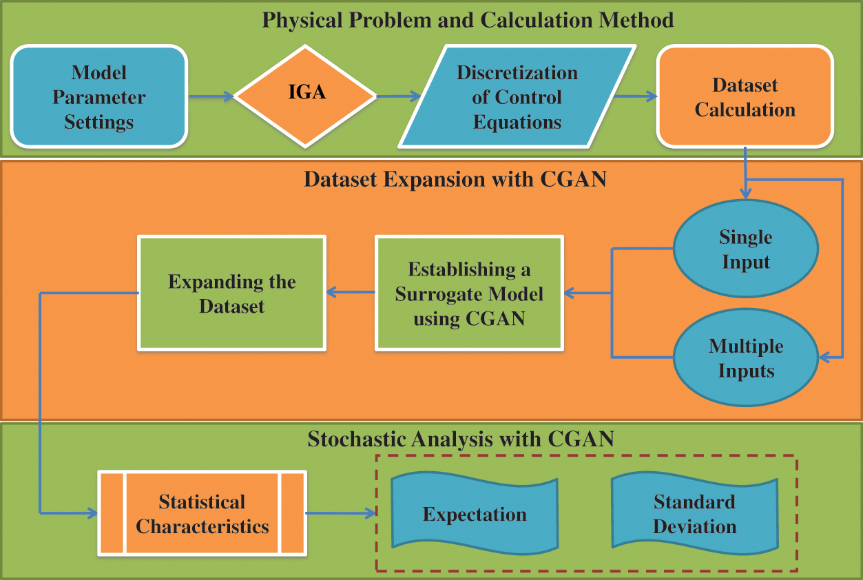
Figure 3: CGAN accelerates the process of uncertainty analysis

3  Theory of Multiphysics Problems

3.1 Theory of Piezoelectricity

In piezoelectric issues, the enthalpy density is usually defined in the following manner:

h(Sij,Ei)=12Cijklεijεkl−ekijEkεij−12κijEiEj.(14)

where Cijkl is the elastic tensor. ekij denotes the dielectric tensor while the κij represents the piezoelectric tensor. The strain tensor εij=12(ui,j+ui,i), and the electric field Ei=−φ,i are defined, with u representing displacement and φ denoting electric potential. The formulation of the governing equation’s weak form concerning piezoelectric issues is presented as follows:

∫ΩCijklδεijεkl{d}Ω+∫Ωekijδφ,kεijdΩ+∫Ωekijφkδεij{d}Ω−∫Ωκijδφ,iφ,j{d}Ω−∫∂Ωf¯iδui{d}Γ−∫ ΓdωδφdΓd=0.(15)

The surface force components f¯i, surface charge density denoted as ω, and the plane Γd where electric loads are applied, are defined within the context. The following section introduces the theoretical formulations for flexoelectric problems, which account for both strain and gradients in the electric field effects.

3.2 Theory of Flexoelectricity

The enthalpy density of dielectric solids, exhibiting flexoelectric effects, depends on both the gradient of strain and the gradient of electric field. This mathematical expression can be articulated as:

ℋ(εij,Ei,εjk,l,Ei,j)=12Cijklεijεkl−eiklEiεkl+(dijklEi,jεkl+fijklEiεjk,l)−12κijEiEj(16)

where the fourth-order direct flexoelectric tensor is denoted by fijkl, and the fourth-order converse flexoelectric tensor is represented by dijkl. Through integration across the physical domain Ω in the aforementioned equation, applying integration by parts and the Gauss divergence theorem to the initial term yields the following result:

∫Ω(dijklEi,jSkl+fijklEiSjk,l)dΩ=−∫Ω(diljk−fijkl)EiSjk,ldΩ+∫∂ΩdijklEiSkldΓ=−∫ΩμijklEiSjk,ldΩ+∫∂ΩdijklEiSkldΓ(17)

where μijkl represents a single material tensor, given by μijkl=diljk−fijkl. Consequently, the Eq. (16) can be rewritten as follows:

ℋ(εij,Ei,εjk,l)=12Cijklεijεkl−eiklEiεkl−μijklEiεjk,l−12κijEiEj.(18)

Comparing Eqs. (15) and (18), it can be seen that the enthalpy density for the flexoelectric problems is similar to the piezoelectric problems. Hence, a corresponding weak formulation of the governing equation for flexoelectric issues can be derived as follows:

∫Ω(Cijklδεijεkl−ekijEkδεij−μlijkElδεij,k−κijδEiEj−eiklδEiεkl−μijklδEiεjk,l)dΩ−∫∂Ωf¯iδuidΓt+∫ΓωδφdΓD=0.(19)

For more details refer to the work of Ghasemi et al. [53].

4  IGA Discretization of Multiphysics Problems

The set of B-spline basis functions Ni,pi=1n is defined over a set of non-decreasing coordinates Ξ=[ξ0,ξ1,…,ξm], the quantity n represents the number of basis functions, while p denotes the order of the polynomial, where m=n+p+1 in the parameter space. Fig. 4 illustrates the partition of unity and the non-negativity properties of these basis functions. The Cox-de-Boor recursive formula is expressed as follows:

Figure 4: An illustration of B-spline shape functions defined by customized knot vectors

Ni,0(ξ)={1ifξi≤ξ<ξi+10otherwiseNi,p(ξ)=ξ−ξiξi+p−ξiNi,p−1(ξ)+ξi+p+1−ξξi+p+1−ξi+1Ni+1,p−1(ξ)(20)

The B-spline surface is defined by the parameter coordinate ξ, with n representing the number of basis functions and p indicating their order. Here, the formula for B-spline surfaces is expressed:

S(ξ,η)=∑i=1n∑j=1mNi,p(ξ)Mj,q(η){P}i,j(21)

The univariate B-spline basis functions of order p and q are denoted as Ni,p(ξ) and Mj,q(η), respectively. The control points of the NURBS surface, represented by Pi,j∈Rd, are also specified. Referring to the B-spline, NURBS surfaces are represented in the following form:

S¯(ξ,η)=∑i=1n∑j=1mRi,jp,q(ξ,η)Pi,j(22)

and

Ri,jp,q(ξ,η)=Ni,p(ξ)Mj,q(η)𝒲i,j∑i′=1n∑j′=1mNi′,p(ξ′)Mi′,q(η)𝒲i′,j′(23)

where ith weight is denoted as 𝒲i. In this investigation, NURBS basis functions are employed for estimating both displacements, denoted as u, and electric potential, denoted as φ.

u=∑B=0nb−1NBUBφ=∑B=0nb−1NBΦB(24)

The displacement coefficients for set Bth are represented by {U}B, while the electric potential node coefficients are denoted as Bth. Here, the total number of basis functions is defined as nb. Utilizing the Bubnov-Galerkin approach, the matrix representation of the weak formulation concerning governing Eq. (15) for multiphysics dilemmas is structured as follows:

[AuuAuφAφuAφφ][uΦ]=[fufφ](25)

and

Auu=∑e∫Ωe(Bu)TC(Bu)dΩe(26)

Auφ=∑e∫Ωe[(Bu)TeT(Bφ)+(Hu)TμT(Bφ)]dΩe(27)

Aφu=∑e∫Ωe[(Bφ)Te(Bu)+(Bφ)Tμ(Hu)]dΩe(28)

Aφφ=−∑e∫Ωe(Bφ)Tκ(Bφ)dΩe(29)

fu=∑e∫∂ΩeNuTf¯idΓe(30)

fφ=−∑e∫ΓDeNφTωdΓDe(31)

where the subscript e in Eqs. (26)–(31) denotes the number of elements.

For piezoelectric problems, the second terms are not contained in Eqs. (27) and (28) and the elastic, piezoelectric, and dielectric matrices are:

C=[C1111C11330C1133C3333000C1313](32)

e=[00e115e311e3330](33)

κ=[κ1100κ22](34)

μ=[μ11μ1200μ44000μ44μ12μ110](35)

For flexoelectric problems, considering the plane strain hypothesis, thus the elastic matrix can be expressed as:

{C}=(Y(1+ν)(1−2ν))[1−νν0ν1−ν000(12−ν)](36)

The variable Y signifies Young’s modulus, while ν represents the Poisson’s ratio in the given context. The Bu, Bφ, and Hu are specified as follows:

Bu=[∂N1∂x∂N2∂x⋯∂Nncp∂x000⋯00⋯0∂N1∂z∂N2∂z⋯∂Nncp∂z∂N1∂z∂N2∂z⋯∂Nncp∂z∂N1∂x∂N2∂x⋯∂Nncp∂z](37)

Bφ=[∂N1∂x⋯∂Nncp∂x∂N1∂z⋯∂Nncp∂z](38)

Hu=[∂2N1∂x2∂2N2∂x2⋯∂2Nncp∂x200⋯000⋯0∂2N1∂z∂x∂2N2∂z∂x⋯∂2Nncp∂z∂x∂2N1∂z∂x∂2N2∂z∂x⋯∂2Nncp∂z∂x∂2N1∂x2∂2N2∂x2⋯∂2Nncp∂x2∂2N1∂x∂z∂2N2∂x∂z⋯∂2Nncp∂x∂z00⋯000⋯0∂2N1∂z2∂2N2∂z2⋯∂2Nncp∂z2∂2N1∂z2∂2N2∂z2⋯∂2Nncp∂z2∂2N1∂x∂z∂2N2∂x∂z⋯∂2Nncp∂x∂z](39)

IGA provides a robust framework for both shape optimization and uncertainty quantification by utilizing NURBS for geometry representation. This integration allows for precise control over geometry, facilitating efficient shape modifications and accurate evaluation of performance metrics. Uncertainty quantification involves assessing the impact of input parameter uncertainties on the model’s output to ensure the robustness and reliability of the results.

5  Numerical Examples

In the following section, the accuracy verification is conducted for the proposed method using two numerical examples. Primarily, uncertainty quantification is utilized to analyze the impact of material parameters on the electric potential of the model. Subsequently, a shape optimization example is introduced where the maximum electric potential of the model is chosen as the optimization objective. The goal is to identify the shape when the electric potential of the model is maximum. Finally, the CGAN is employed to establish a correlation between the material parameters and the electric potential of the optimal model to perform uncertainty quantification for optimal models under uncertain conditions.

5.1 Piezoelectric Clamped Tapered Panel

5.1.1 The Static Analysis Focuses on Clamped Tapered Panels with Piezoelectric Properties

This section focuses on performing a static analysis of the clamped tapered panel depicted in Fig. 5. The left boundary of the tapered piezoelectric panel was secured, while the right boundary experienced a distributed load. Additionally, the bottom edge was set to have a zero electric potential. The boundary conditions are chosen to be similar to the cantilever structure. The model is built using Lead Zirconate Titanate-4 (PZT-4) piezoelectric material, with the specific material parameters listed in Table 1. Additionally, a zero electric potential is assigned to the lower surface. IGA employs NURBS functions from CAD as shape functions, which can accurately represent geometric models. Using h-refinement will significantly increase the number of control points, adding to the computational burden. Therefore, p-refinement can be adopted to improve numerical accuracy by increasing the order of the basis functions, as demonstrated in the second example in this paper. In the piezoelectric example, the accuracy gap between finite element method and IGA calculations is not significant. However, for flexoelectric problems, due to the need to consider the impact of strain gradients, finite element method is not suitable for solving flexoelectric problems, thus, this paper considers the IGA method. In contrast, the IGA approach employed first-order NURBS basis functions for piezoelectric material examples to facilitate rapid computations while maintaining accuracy. Due to the flexoelectric effect requiring consideration of the strain gradient, first-order NURBS basis functions are not suitable. Therefore, this paper employs the p-refinement method, increasing the basis functions to second-order.

Figure 5: A schematic illustrating the layout of a model featuring a clamped tapered panel

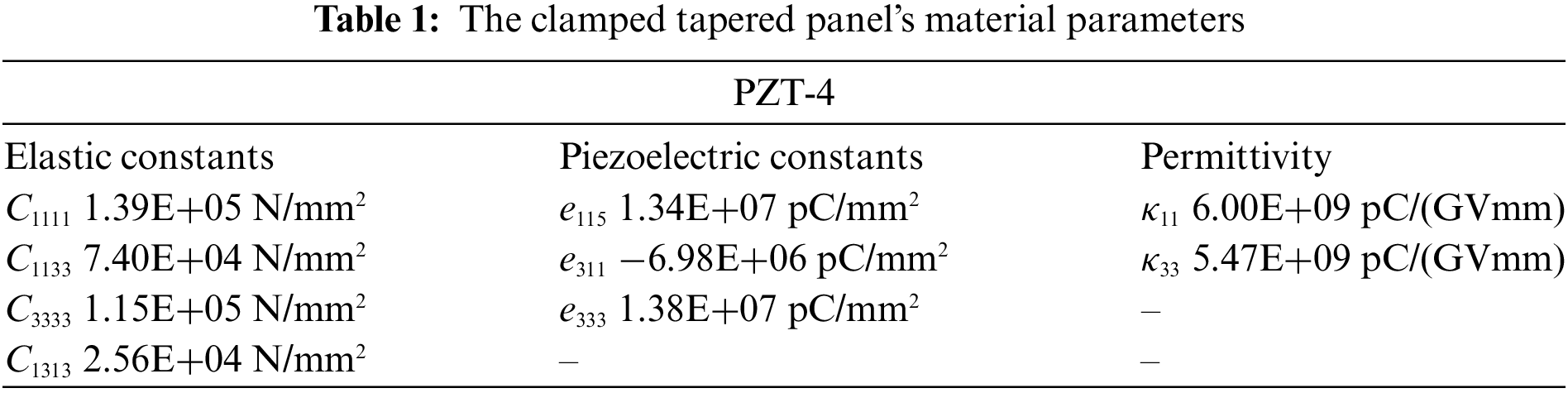
Fig. 6 illustrates the electric potential distribution of a clamped tapered panel, taking into account piezoelectric effects, alongside the h-refinement model of the clamped tapered panel computed using the IGA method.

Figure 6: The electric potential results using h-refinement. (a) The h-refinement model, (b) the electric potential result

5.1.2 Verification of CGAN Method in Piezoelectric Problems

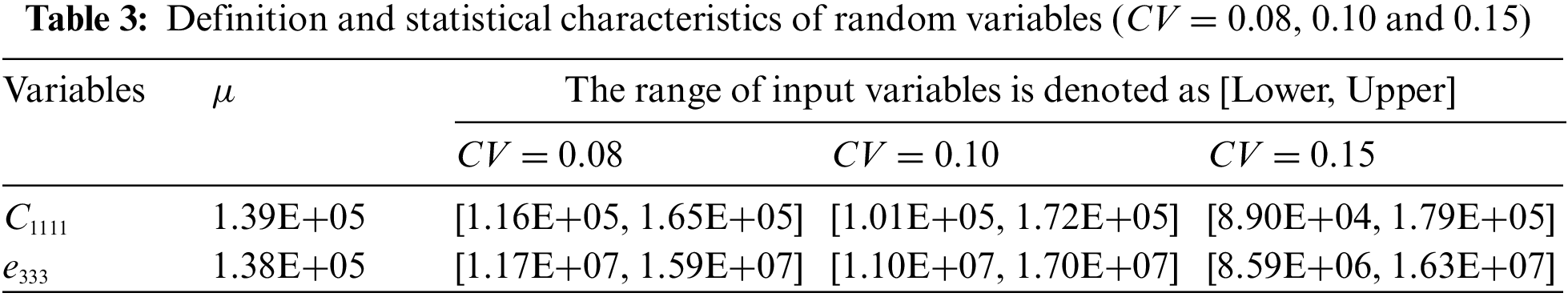
In the subsequent section, the model discussed earlier is adopted to validate the efficacy of the CGAN method. The random input variables examined are the elastic constant C1111 and the piezoelectric constant e333. These random variables follow Gaussian distributions with expected values μ = 1.39E+05 and μ = 1.38E+07, respectively. The coefficient of variation, denoted by CV, is used to calculate the standard deviation, given as σ=μ×CV.

Tables 2 and 3 present details of input parameters. Using the 3σ principle, the range of the datasets is established. For single random input variables (“1-D”), a total of 100 sampling points, labeled as na, are selected. However, for multidimensional input variables (“2-D”), na is chosen as 102. Finding a balance in the number of sampling points for Monte Carlo simulation is crucial because computational efficiency is dependent on the quantity of sampling points. Insufficient sample points may compromise computational accuracy, while an excess of sample points reduces computational efficiency. Subsequently, 100 samples are obtained using IGA for transmission to CGAN for training purposes, thereby expanding the sample set. Eighty samples were chosen from the total of 100 for training purposes, leaving the remaining 20 for testing. Both the generator and discriminator utilize fully connected neural networks comprising three hidden layers. The dimensionality of the noise vector matches that of the label, and the Adam optimization algorithm is employed. To achieve precise data fitting, the loss function is defined as binary cross-entropy, with the learning rate configured to 0.0002. The training process consists of 5000 sessions.

The predicted results for both the “1-D” and “2-D” analyses can be observed in Figs. 7–9. The consistency between the results derived from the CGAN method and those from IGA is evident. The results obtained from CGAN-IGA demonstrate the effectiveness of CGAN as a sample extension method, indicating its capability to effectively predict the response of piezoelectric problems.

Figure 7: Electric potential results obtained from CGAN and IGA (C1111)

Figure 8: Electric potential results obtained from CGAN and IGA (e333)

Figure 9: Electric potential results obtained from CGAN and IGA (C1111 + e333)

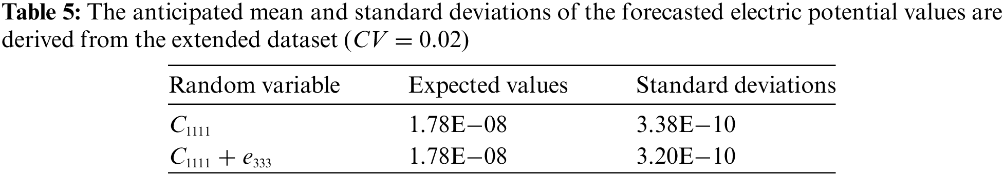
5.1.3 Uncertainty Quantification Based on Optimal Clamped Tapered Panel Model under Uncertain Parameters

In this section, the shape optimization analysis of the model in Section 5.1.1 is performed using different parameters to obtain the optimal models that maximize the electric potential. Then, the electric potential variations are examined for the optimized model under uncertain parameters. Precisely, the initial sample is computed based on the parameters outlined in the preceding section. Consequently, a dataset with a size of 100 × 100 using the IGA method is obtained and the electric potential of piezoelectric problems is calculated using the dataset, followed by training the CGAN. For each parameter sample, the optimized model with maximum electric potential corresponding to one hundred parameter sets is obtained. Ultimately, a prediction model is established using different random parameters to conduct the uncertainty quantification.

To perform shape optimization, adjustments are made to the coordinates of the control points located at the top and bottom of the right edge of the model, enabling variations within a range of 10%. To obtain samples, the Latin hypercube sampling is adopted. Later, to verify the fitting capability of CGAN, the tests on the dataset are performed. To optimize the shape of the model using uncertainty parameters, each adjustment in the parameters undergoes a shape optimization process. However, when the coefficient of variation is 0.02, the influence of random variables on electric potential is insignificant. Hence, to conserve computational resources, the shape optimization analysis is performed on uncertain parameters using a coefficient of variation of 0.02. The objective of this analysis was to investigate how alterations in shape affect the electric potential. The optimal shape coordinates are derived by leveraging predictive models and incorporating uncertainty parameters. Additionally, the sample set from 100 to 2000 samples is expanded to conduct a more comprehensive analysis. Table 4 shows the improvement of maximum electric potential before and after optimization. In Table 4, P1 and P2 represent the coordinates of two points located on the right side of the example. The electric potentials recorded in the table are the values at the midpoint of the line connecting P1 and P2, providing a direct measure of the electric potential magnitude within the model. Subsequently, the optimization model in Scenario 4 is employed using different random parameters to obtain their electric potential, facilitating uncertainty quantification through the CGAN-IGA method. In Fig. 10, the electric potential’s predicted values from the optimization model with various random parameters are depicted. Observing Fig. 10, a gradual decrease in the maximum potential linked with the optimized model is evident with the increment of C1111. Moreover, the rise in e333 results in a higher maximum electric potential observed in the optimized model, especially when considering the interplay of two random variables, C1111 and e333. Table 5 presents the anticipated values and standard deviations of the electric potential for optimal models utilizing an expanded dataset with a coefficient of variation set at 0.02. These findings underscore the suitability of CGAN-IGA for effectively quantifying uncertainties in piezoelectric problems. According to reference [54], under the boundary conditions of scenario 1, the analytical solution for the electric potential at the midpoint of the line connecting points P1 and P2 on the right side of a piezoelectric clamped tapered panel is 1.73E−08V. The reference solution obtained in this paper is 1.72E−08V, with a difference of 0.5%, thereby verifying the correctness of the solution in this paper.

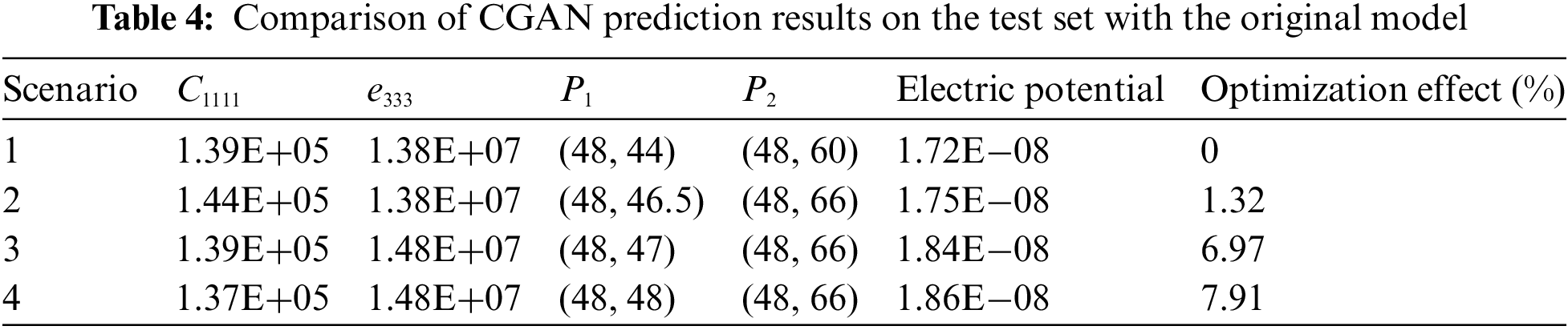
Figure 10: (a and b) show the values predicted of electric potential using CGAN under the change in parameters C1111 and C1111+e3333, respectively

5.2 Flexoelectric Truncated Pyramid

5.2.1 Static Analysis of Truncated Pyramid

The truncated pyramid model is often used model in flexoelectric problems because the model can generate significant strain gradients under excitation. Therefore, the model selected for examination in this section is the one depicted. The meshing of the truncated pyramid model, depicted in Fig. 11, is shown. The bottom edge of the pyramid remains stationary, while a consistent force with strength F acts upon its top edge. Table 6 provides the material parameters and dimensions used in the model. By using the IGA method, the electric potential is obtained as shown in Fig. 12.

Figure 11: (a) illustrates the application of a uniformly distributed force denoted as F to the upper edge of the truncated pyramid model. (b) depicts the discretization meshing of the model

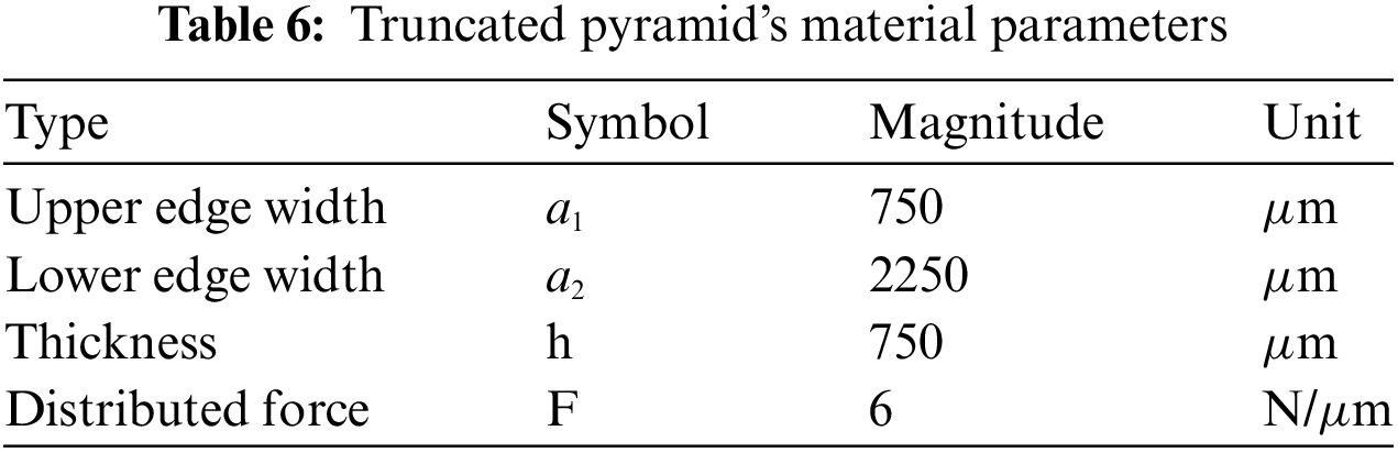
Figure 12: (a) illustrates the distribution of overall electric potential φ, while (b) provides the mesh information

5.2.2 Verification of CGAN Method in Flexoelectric Problems

The verification process for the CGAN method in flexoelectric problems is carried out similarly to the previous example. Second-order NURBS basis functions were used for flexoelectric material examples to enhance the geometric representation and solution continuity. Selected randomly as input parameters are Young’s modulus denoted as Y and a force uniformly distributed, labeled as F. The range of variation and statistical characteristics of these parameters are presented in Tables 7 and 8. The designated output variable is the maximum electric potential observed at the lower edge.

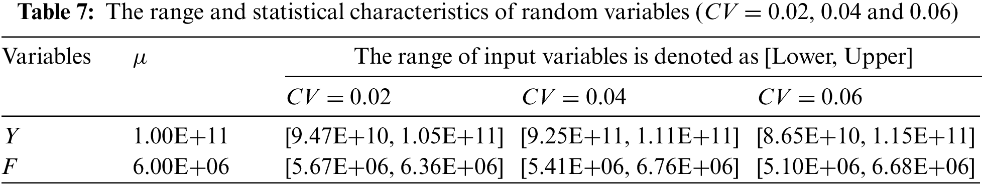
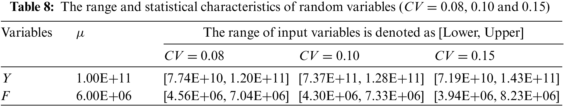
Fig. 13 illustrates a comparison of the electric potential produced by the material under excitation, demonstrating outcomes from both CGAN and IGA methods. Young’s modulus is utilized as a stochastic input parameter for uncertainty quantification purposes. The comparison results demonstrate the agreement between the results obtained from IGA and CGAN simulations, indicating the effectiveness of the algorithm. Moreover, the results present the significant role played by Young’s modulus in determining the potential generated by material excitation. The observed discrepancy can be ascribed to the impact of Young’s modulus on the structural stiffness, consequently influencing the resulting electric potential. A comparative analysis of the electric potential, derived from both CGAN and IGA approaches, is illustrated in Fig. 14, considering a uniformly distributed force as a stochastic parameter. The graph illustrates a rise in the electric potential’s intensity with the increase in the uniformly distributed force. In this analysis, both Young’s modulus and the uniformly distributed force are treated as stochastic input parameters. To delve deeper into the mechanical characteristics of flexoelectric material, Fig. 15 illustrates the comparative outcomes of CGAN and IGA. Significantly, CGAN exhibits the ability to establish a surrogate model concerning mechanical characteristics, even when dealing with a limited dataset, thereby guaranteeing accuracy in computations. This distinguishing feature distinguishes CGAN from conventional uncertainty quantification techniques, such as MCs.

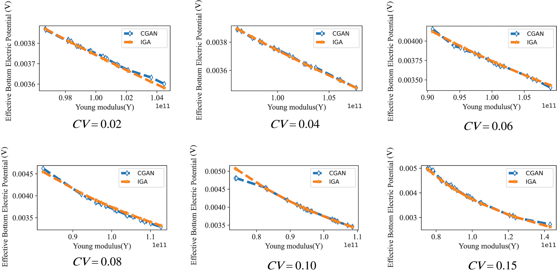
Figure 13: Predicted values of the electric potential of truncated pyramid model under different coefficients of variation using Young’s modulus Y

Figure 14: The anticipated electric potential values of the truncated pyramid model are examined under various coefficients of variation across distinct distributed force scenarios F

Figure 15: The anticipated electric potential values of the truncated pyramid model are evaluated across various coefficients of variation, considering different combinations of Young’s modulus Y and uniformly distributed force F

5.2.3 Uncertainty Quantification Based on Optimal Truncated Pyramid Model under Uncertain Parameters

Similar to Section 5.1.3, the influence of parameter variations on the shape of the flexoelectric model is investigated using Young’s modulus Y and uniformly force F in this section to obtain the optimal model. Subsequently, the optimal model is employed to perform uncertainty quantification. To be specific, adjustments are made to the horizontal coordinates of control points along the left and right edges of the truncated pyramid model, within a 20% range. The control points of the model are depicted in Fig. 16, with the optimized area of control points indicated by the red dashed box. All other arrangements of the example remain consistent with the truncated pyramid model in Section 5.2.1.

Figure 16: The control points of the truncated pyramid IGA model where the control points inside the red dashed box are optimized using the CGAN method

To verify the generalization ability of CGAN, 80% of the dataset for training are allocated and the remaining 20% for testing are retained. The discrepancy between the predicted values obtained from the test results and those derived from the IGA results is less than 2%. The shape optimization analysis of a truncated pyramid model with uncertain parameters using a coefficient of variation of 0.02 is conducted. The optimal shape coordinates of the model are obtained by changing uncertainty parameters and expanding the sample set from 100 samples to 2000 samples. In Table 9, the anticipated enhancements in the maximum electric potential are presented, both pre and post optimization. Fig. 17 shows the electric potential distribution corresponding to the parameters in Table 9, and Fig. 18 displays the shape and control points of the model post-optimization, while in Fig. 19, the shape and control points of the model after optimization are depicted. Fig. 19 gives the predicted values of the electric potential of the optimal model in Scenario 4 using the different Young’s modulus Y, uniformly force F, and their combination. A noticeable trend is observed wherein an elevation in Young’s modulus results in a gradual decline in the predicted electric potential values. Conversely, the behavior exhibits the opposite trend for using different uniformly distributed forces. Even when both of these parameters are altered simultaneously, the anticipated electric potential values of the optimized model exhibit a consistent pattern, aligning consistently with our earlier discourse.

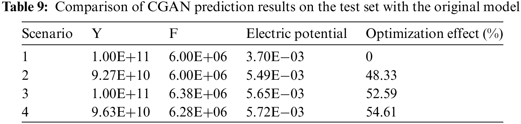
Figure 17: (a–c) Correspond to the electric potential distributions of optimization models of Scenario 2, Scenario 3, and Scenario 4

Figure 18: The shape obtained by Scenario 2, Scenario 3 and Scenario 4 using the CGAN method

Figure 19: The predicted values of electric potential obtained from the CGAN method under changes in parameters Y, F, and Y + F, respectively

6  Conclusions

This research introduces the CGAN-IGA method, a novel computational framework integrating IGA with CGAN, for optimizing the shapes of dielectric solids and quantifying their mechanical uncertainties. Key outcomes of our study include:

1.    Efficiency and Accuracy: IGA’s integration minimizes repetitive meshing, significantly enhancing the efficiency and accuracy of the computational processes involved in uncertainty quantification.

2.    Optimization Acceleration: By incorporating CGAN, the optimization and uncertainty quantification processes under uncertain parameters are expedited, demonstrating a leap in computational speed and reliability.

3.    Empirical Validation: The CGAN-IGA approach has been rigorously tested through several numerical examples, validating its accuracy and confirming its robustness for practical applications.

To address these limitations and further advance the field, subsequent research will focus on:

1.    Enhancing Analytical Techniques: More sophisticated methods will be developed for analyzing materials that exhibit complex behavior due to multidimensional variable influences.

2.    Advancing Surrogate Model Accuracy: Cutting-edge deep-learning strategies will be explored to refine the accuracy and stability of surrogate models, thereby enhancing the dependability of uncertainty quantification efforts.

These initiatives are expected to refine the methodology and extend its applicability to more complex systems, thereby enriching the tools available for materials science and engineering research.

Acknowledgement: The authors wish to express their appreciation to the reviewers for their helpful suggestions which greatly improved the presentation of this paper.

Funding Statement: The authors received no specific funding for this study.

Author Contributions: The authors confirm contribution to the paper as follows: study conception and design: Shuai Li, Xiaodong Zhao; data collection: Shuai Li, Xiaodong Zhao; analysis and interpretation of results: Shuai Li, Jinghu Zhou; draft manuscript preparation: Shuai Li, Xiyue Wang. All authors reviewed the results and approved the final version of the manuscript.

Availability of Data and Materials: All datasets mentioned in the manuscript are included.

Conflicts of Interest: The authors declare that they have no conflicts of interest to report regarding the present study.

References

1. George SP, Isaac J, Philip J. Coupled field analysis of piezoelectric materials for sensor and actuator applications using finite element method. Mater Today Proc. 2022;59(1–3):1202–10. doi:10.1016/j.matpr.2022.03.422. [Google Scholar] [CrossRef]

2. Swain PR, Dash P, Singh BN. Stochastic nonlinear bending analysis of piezoelectric laminated composite plates with uncertainty in material properties. Mech Based Des Struct Mach. 2021;49(2):194–216. doi:10.1080/15397734.2019.1674663. [Google Scholar] [CrossRef]

3. Abuzaid A, Hrairi M, Shaik Dawood M. Survey of active structural control and repair using piezoelectric patches. In: Actuators. Basel, Switzerland: MDPI; 2015. vol. 4, p. 77–98. [Google Scholar]

4. Aabid A, Raheman MA, Ibrahim YE, Anjum A, Hrairi M, Parveez B, et al. A systematic review of piezoelectric materials and energy harvesters for industrial applications. Sensors. 2021;21(12):4145. doi:10.3390/s21124145. [Google Scholar] [PubMed] [CrossRef]

5. Hooper TE, Roscow JI, Mathieson A, Khanbareh H, Goetzee-Barral AJ, Bell AJ. High voltage coefficient piezoelectric materials and their applications. J Eur Ceram Soc. 2021;41(13):6115–29. doi:10.1016/j.jeurceramsoc.2021.06.022. [Google Scholar] [CrossRef]

6. Watson BHIII, Brova MJ, Fanton M, MeyerJr RJ, Messing GL. Textured Mn-doped PIN-PMN-PT ceramics: harnessing intrinsic piezoelectricity for high-power transducer applications. J Eur Ceram Soc. 2021;41(2):1270–9. doi:10.1016/j.jeurceramsoc.2020.07.071. [Google Scholar] [CrossRef]

7. Micheal A, Bahei-El-Din YA. Implementation of multiscale mechanisms in finite element analysis of active composite structures. J Compos Mater. 2022;56(13):2129–44. doi:10.1177/00219983221082492. [Google Scholar] [CrossRef]

8. Majdoub M, Sharma P, Cagin T. Enhanced size-dependent piezoelectricity and elasticity in nanostructures due to the flexoelectric effect. Phys Rev B. 2008;77(12):125424. doi:10.1103/PhysRevB.77.125424. [Google Scholar] [CrossRef]

9. Yudin P, Tagantsev A. Fundamentals of flexoelectricity in solids. Nanotechnology. 2013;24(43):432001. doi:10.1088/0957-4484/24/43/432001. [Google Scholar] [PubMed] [CrossRef]

10. Li H, Zhao J, Guo X, Cheng Y, Xu Y, Yuan X. Sensitivity analysis of flexoelectric materials surrogate model based on the isogeometric finite element method. Front Phys. 2022;10:1343. doi:10.3389/fphy.2022.1111159. [Google Scholar] [CrossRef]

11. Yu D, Wang S, Li W, Yang Y, Hong J. Shape sensing for thin-shell spaceborne antennas with adaptive isogeometric analysis and inverse finite element method. Thin-Walled Struct. 2023;192:111154. doi:10.1016/j.tws.2023.111154. [Google Scholar] [CrossRef]

12. Chen L, Wang Z, Lian H, Ma Y, Meng Z, Li P, et al. Reduced order isogeometric boundary element methods for CAD-integrated shape optimization in electromagnetic scattering. Comput Methods Appl Mech Eng. 2024;419:116654. [Google Scholar]

13. Hughes TJ, Cottrell JA, Bazilevs Y. Isogeometric analysis: CAD, finite elements, NURBS, exact geometry and mesh refinement. Comput Methods Appl Mech Eng. 2005;194(39–41):4135–95. [Google Scholar]

14. Schillinger D, Dede L, Scott MA, Evans JA, Borden MJ, Rank E, et al. An isogeometric design-through-analysis methodology based on adaptive hierarchical refinement of NURBS, immersed boundary methods, and T-spline CAD surfaces. Comput Methods Appl Mech Eng. 2012;249:116–50. [Google Scholar]

15. Chen L, Zhao J, Lian H, Yu B, Atroshchenko E, Li P. A BEM broadband topology optimization strategy based on Taylor expansion and SOAR method–Application to 2D acoustic scattering problems. Int J Numer Meth Eng. 2023;124(23):5151–82. [Google Scholar]

16. Venås JV, Kvamsdal T. Isogeometric boundary element method for acoustic scattering by a submarine. Comput Methods Appl Mech Eng. 2020;359:112670. [Google Scholar]

17. Wu Y, Dong C, Yang H. Isogeometric FE-BE coupling approach for structural-acoustic interaction. J Sound Vib. 2020;481(5):115436. doi:10.1016/j.jsv.2020.115436. [Google Scholar] [CrossRef]

18. Wang Y, Liao Z, Shi S, Wang Z, Poh LH. Data-driven structural design optimization for petal-shaped auxetics using isogeometric analysis. Comput Model Eng Sci. 2020;122(2):433–58. doi:10.32604/cmes.2020.08680. [Google Scholar] [CrossRef]

19. Zhang K, Cheng G. Structural topology optimization with four additive manufacturing constraints by two-phase self-supporting design. Struct Multidiscip Optim. 2022;65(11):339. doi:10.1007/s00158-022-03366-y. [Google Scholar] [CrossRef]

20. Cao G, Yu B, Chen L, Yao W. Isogeometric dual reciprocity BEM for solving non-Fourier transient heat transfer problems in FGMs with uncertainty analysis. Int J Heat Mass Transfer. 2023;203(6):123783. doi:10.1016/j.ijheatmasstransfer.2022.123783. [Google Scholar] [CrossRef]

21. Chen L, Lian H, Liu Z, Gong Y, Zheng C, Bordas S. Bi-material topology optimization for fully coupled structural-acoustic systems with isogeometric FEM-BEM. Eng Anal Bound Elem. 2022;135(1):182–95. doi:10.1016/j.enganabound.2021.11.005. [Google Scholar] [CrossRef]

22. Zhang S, Yu B, Chen L. Non-iterative reconstruction of time-domain sound pressure and rapid prediction of large-scale sound field based on IG-DRBEM and POD-RBF. J Sound Vib. 2024;573:118226. doi:10.1016/j.jsv.2023.118226. [Google Scholar] [CrossRef]

23. Chen L, Lian H, Dong H, Yu P, Jiang S, Bordas SP. Broadband topology optimization of three-dimensional structural-acoustic interaction with reduced order isogeometric FEM/BEM. J Comput Phys. 2024;509(9):113051. doi:10.1016/j.jcp.2024.113051. [Google Scholar] [CrossRef]

24. Liu Z, Yang M, Cheng J, Tan J. A new stochastic isogeometric analysis method based on reduced basis vectors for engineering structures with random field uncertainties. Appl Math Model. 2021;89(1–2):966–90. doi:10.1016/j.apm.2020.08.006. [Google Scholar] [CrossRef]

25. Ghasemi H, Park HS, Alajlan N, Rabczuk T. A computational framework for design and optimization of flexoelectric materials. Int J Comput Methods. 2020;17(1):1850097. doi:10.1142/S0219876218500974. [Google Scholar] [CrossRef]

26. Abdollahi A, Peco C, Millan D, Arroyo M, Arias I. Computational evaluation of the flexoelectric effect in dielectric solids. J Appl Phys. 2014;116(9):435. doi:10.1063/1.4893974. [Google Scholar] [CrossRef]

27. Liu TW, Bai JB, Xi HT, Fantuzzi N. A curved bistable composite slit tube for deployable membrane structures. Compos Commun. 2023;41(12):101648. doi:10.1016/j.coco.2023.101648. [Google Scholar] [CrossRef]

28. Ahmadpoor F, Sharma P. Flexoelectricity in two-dimensional crystalline and biological membranes. Nanoscale. 2015;7(40):16555–70. doi:10.1039/C5NR04722F. [Google Scholar] [PubMed] [CrossRef]

29. Qu Y, Guo Z, Zhang G, Gao XL, Jin F. A new model for circular cylindrical Kirchhoff-Love shells incorporating microstructure and flexoelectric effects. J Appl Mech. 2022;89(12):121010. doi:10.1115/1.4055658. [Google Scholar] [CrossRef]

30. Avey M, Fantuzzi N, Sofiyev A, Zamanov A, Hasanov Y, Schnack E. Buckling behavior of multilayer cylindrical shells composed of functionally graded nanocomposite layers under lateral pressure in thermal environments. Compos Part C: Open Access. 2023;12(9):100417. doi:10.1016/j.jcomc.2023.100417. [Google Scholar] [CrossRef]

31. Pu H, Xu Y, Huo Y. Analysis of the effect of nominal electric field strength and axial constraint on electric-field-induced bending of dielectric liquid crystal elastomers. Chin Q Mech. 2022;43(4):751. [Google Scholar]

32. Shen X, Du C, Jiang S, Zhang P, Chen L. Multivariate uncertainty analysis of fracture problems through model order reduction accelerated SBFEM. Appl Math Model. 2024;125(3–4):218–40. doi:10.1016/j.apm.2023.08.040. [Google Scholar] [CrossRef]

33. Zuo G, Hou L, Lin R, Ren S, Chen Y. Combination resonance and primary resonance characteristics of a dual-rotor system under the condition of the synchronous impact of the inter-shaft bearing. Sci Rep. 2023;13(1):1153. doi:10.1038/s41598-023-27922-8. [Google Scholar] [PubMed] [CrossRef]

34. Fantuzzi N, Vidwans A, Dib A, Trovalusci P, Agnelli J, Pierattini A. Flexural characterization of a novel recycled-based polymer blend for structural applications. In: Structures. Amsterdam, Netherlands: Elsevier; 2023. vol. 57, p. 104966. [Google Scholar]

35. Chen L, Cheng R, Li S, Lian H, Zheng C, Bordas SP. A sample-efficient deep learning method for multivariate uncertainty qualification of acoustic-vibration interaction problems. Comput Methods Appl Mech Eng. 2022;393(5):114784. doi:10.1016/j.cma.2022.114784. [Google Scholar] [CrossRef]

36. Chen L, Lian H, Natarajan S, Zhao W, Chen X, Bordas S. Multi-frequency acoustic topology optimization of sound-absorption materials with isogeometric boundary element methods accelerated by frequency-decoupling and model order reduction techniques. Comput Methods Appl Mech Eng. 2022;395(4):114997. doi:10.1016/j.cma.2022.114997. [Google Scholar] [CrossRef]

37. Jahanbin R, Rahman S. Stochastic isogeometric analysis in linear elasticity. Comput Methods Appl Mech Eng. 2020;364(4):112928. doi:10.1016/j.cma.2020.112928. [Google Scholar] [CrossRef]

38. Sun K, Liang Y, Cheng G. Sensitivity analysis of discrete variable topology optimization. Struct Multidiscip Optim. 2022;65(8):216. doi:10.1007/s00158-022-03321-x. [Google Scholar] [CrossRef]

39. Chen L, Lian H, Xu Y, Li S, Liu Z, Atroshchenko E, et al. Generalized isogeometric boundary element method for uncertainty analysis of time-harmonic wave propagation in infinite domains. Appl Math Model. 2023;114(39–41):360–78. doi:10.1016/j.apm.2022.09.030. [Google Scholar] [CrossRef]

40. Liu T, Bai J, Fantuzzi N. Analytical model for predicting folding stable state of bistable deployable composite boom. Chin J Aeronaut. 2023;36:107178. [Google Scholar]

41. Liu TW, Bai JB, Fantuzzi N. Analytical models for predicting folding behaviour of thin-walled tubular deployable composite boom for space applications. Acta Astronaut. 2023;208(7–8):167–78. doi:10.1016/j.actaastro.2023.04.012. [Google Scholar] [CrossRef]

42. Goodfellow I, Pouget-Abadie J, Mirza M, Xu B, Warde-Farley D, Ozair S, et al. Generative adversarial nets. Adv Neural Inf Process Syst. 2014;27:1–9. [Google Scholar]

43. Oishi A, Yagawa G. Computational mechanics enhanced by deep learning. Comput Methods Appl Mech Eng. 2017;327:327–51. [Google Scholar]

44. Papadrakakis M, Lagaros ND. Reliability-based structural optimization using neural networks and Monte Carlo simulation. Comput Methods Appl Mech Eng. 2002;191(32):3491–507. [Google Scholar]

45. LeCun Y, Bengio Y, Hinton G. Deep learning. Nature. 2015;521(7553):436–44. [Google Scholar] [PubMed]

46. Jin Y, Hou L, Zhong S, Yi H, Chen Y. Invertible Koopman network and its application in data-driven modeling for dynamic systems. Mech Syst Signal Process. 2023;200:110604. [Google Scholar]

47. Zhang H, Xu T, Li H, Zhang S, Wang X, Huang X, et al. StackGAN++: realistic image synthesis with stacked generative adversarial networks. IEEE Trans Pattern Anal Mach Intell. 2018;41(8):1947–62. [Google Scholar] [PubMed]

48. Liu Y, Zhang J, Zhao T, Wang Z, Wang Z. Reconstruction of the meso-scale concrete model using a deep convolutional generative adversarial network (DCGAN). Constr Build Mater. 2023;370:130704. [Google Scholar]

49. Antoniou A, Storkey A, Edwards H. Data augmentation generative adversarial networks. arXiv preprint arXiv:171104340; 2017. [Google Scholar]

50. Jain P, Kar P. Non-convex optimization for machine learning. Found Trends Mach Learn. 2017;10(3–4):142–363. [Google Scholar]

51. Samaniego E, Anitescu C, Goswami S, Nguyen-Thanh VM, Guo H, Hamdia K, et al. An energy approach to the solution of partial differential equations in computational mechanics via machine learning: concepts, implementation and applications. Comput Methods Appl Mech Eng. 2020;362:112790. [Google Scholar]

52. Jin Y, Hou L, Lu Z, Chen Y. Crack fault diagnosis and location method for a dual-disk hollow shaft rotor system based on the radial basis function network and pattern recognition neural network. Chin J Mech Eng. 2023;36(1):35. [Google Scholar]

53. Ghasemi H, Park HS, Rabczuk T. A level-set based IGA formulation for topology optimization of flexoelectric materials. Comput Methods Appl Mech Eng. 2017;313:239–58. [Google Scholar]

54. Li H, Chen L, Zhi G, Meng L, Lian H, Liu Z, et al. A direct FE2 method for concurrent multilevel modeling of piezoelectric materials and structures. Comput Methods Appl Mech Eng. 2024;420:116696. [Google Scholar]