MADDPG-D2: An Intelligent Dynamic Task Allocation Algorithm Based on Multi-Agent Architecture Driven by Prior Knowledge

1  Introduction

Dynamic Task Allocation (DTA) refers to the rational assignment of a certain type and number of platforms on one’s side according to factors such as the allocation purpose, environment situation, and equipment performance to achieve efficient interception of incoming attack targets [1–3]. At present, with the continuous development of the Internet of Things, big data, and artificial intelligence technology, the difficulty of DTA is getting bigger and bigger [4]. How to carry out DTA more accurately and efficiently has become a task to be solved [5–8]. In recent years, researchers at home and abroad have put forward many methods to solve the DTA problem, among which the classical methods mainly include traditional methods [9,10] and bionic intelligent algorithms [11–14].

The above-mentioned algorithms have made some achievements in each stage, but they are difficult to adapt to in a complex and changeable dynamic environment because of their lack of awareness of the environment. As a result, these methods make it difficult to perform efficient DTA in the absence of a priori knowledge and dynamic environments.

Reinforcement learning (RL) does not need to build an environment model, and the agent carries out trial and error learning through continuous interaction with the environment until it has good DTA capability [15,16]. The deep reinforcement learning (DRL) algorithm can realize the end-to-end learning process from perception to action, and its learning mechanism and method fit the empirical learning and decision-making mindset of combat commanders, and they have obvious advantages for solving sequential decision-making problems under game-confrontation conditions [17,18]. Zhang et al. conducted a target situation assessment through RL, and used the actor-critic (AC) algorithm to effectively estimate the expected effect of missile attacks under the current situation [19]; Aiming at the unmanned aerial vehicle (UAV) short-range air combat problem, Yang et al. established a maneuvering decision model including UAV motion model, one-to-one short-range air combat evaluation model and Deep Q network (DQN) based maneuver decision model based on DRL theory [20]; Fu et al. put forward an agent training framework to solve the problem of DTA, aiming at solving the dynamic decision-making problem of air defense combat in complex environment through the method of RL learning training [21]; On this basis, Liu et al. improved the training framework, and based on the idea of optimal algorithm of allocation strategy, proximal policy optimization (PPO) algorithm was used to train and solve the agent [22].

However, the above research mainly focuses on the single-agent method and simple scenarios. Although this method has a great global coordination ability, with the increase of combat entities and the gradual complexity of the environment situation, the state and action space will increase exponentially, and the decision-making process will face a high-dimensional state-action space. In this case, if all the entities are simply regarded as agents, it will lead to problems such as problematic convergence of the model and poor decision-making effect. Therefore, the multi-agent algorithm based on multi-agent architecture should be considered. Compared with other algorithms, the Multi-Agent Deep Deterministic Policy Gradient (MADDPG) algorithm can be applied to a variety of task scenarios, such as competition and cooperation among multi-agents, and at the same time, it can use the observation information of other agents for centralized training, thus improving the efficiency of the algorithm, and adopting the mechanism of policy inference and policy collection to enhance the robustness of the algorithm, and the application scenario is broader [23].

In summary, this paper considers the multi-agent algorithm based on multi-agent architecture to solve the large-scale weapon-target assignment problem. Based on the theory of DRL, a multi-agent architecture for intelligent DTA is constructed, which is solved by the Multi-Agent Deep Deterministic Policy Gradient algorithm with a dual experience replay pool and a dual noise (MADDPG-D2) algorithm. At the same time, the training of agents is accelerated by fusing prior knowledge with experts to improve the decision-making ability of intelligent DTA in large-scale and complex environments. Finally, the method is deduced and verified on the ground-to-air confrontation digital simulation platform, and the experimental results prove the effectiveness of the method used in this paper.

The main contributions of our work are as follows:

1.   First, an intelligent DTA framework based on multi-agent reinforcement learning (MARL) algorithms is proposed, which adopts the training paradigm of “centralized training and distributed execution (CTDE)” to better overcome the non-stationarity of the environment and continuously improve the training efficiency.

2.   Second, in order to increase the action exploration space of the MADDPG algorithm and improve the utilization of data, the MADDPG-D2 algorithm is proposed by considering the introduction of the dual experience pool mechanism and dual noise mechanism into the traditional MADDPG algorithm.

3.   Finally, to overcome the “cold start” problem of the MADDPG algorithm in the training process and accelerate the training of the algorithm, a pre-training process is introduced in the initial stage of the algorithm training, which improves the initial solving capability of the MADDPG-D2 algorithm.

This paper is organized as follows: Section 2 reviews the Multi-Agent System (MAS) and MADDPG algorithm, and introduces the principle of the MADDPG-D2 algorithm; Section 3 describes the state space, action space, and reward function in Partially observable Markov decision process (POMDP), and Section 4 outlines the experimental environment, simulation architecture, hyper-parameter setting, and network structure. Section 5 evaluates the results of the experiment and concludes that the proposed model and algorithm are effective when facing large-scale DTA problem, which provide ideas for solving such problems. Section 6 is the conclusion.

2  Background

2.1 Multi-Agent System

MAS is a system composed of multiple interactive entities in the same environment, which has the characteristics of modularity, extensibility, parallelism, and strong robustness. It is often used to solve problems that are difficult to solve with a single agent system.

Figs. 1 and 2 are multi-agent architecture and single-agent architecture, respectively.

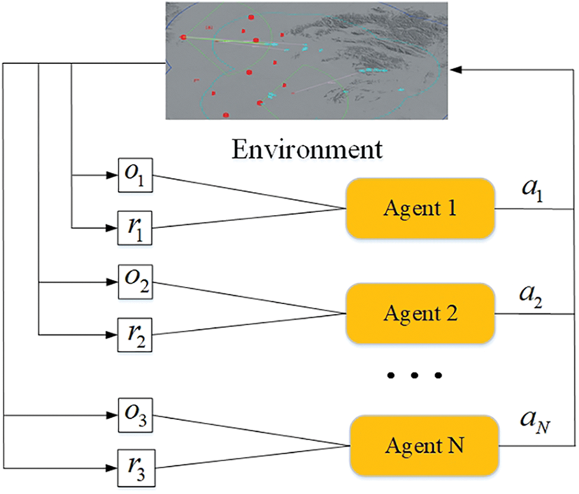
Figure 1: Multi-agent architecture

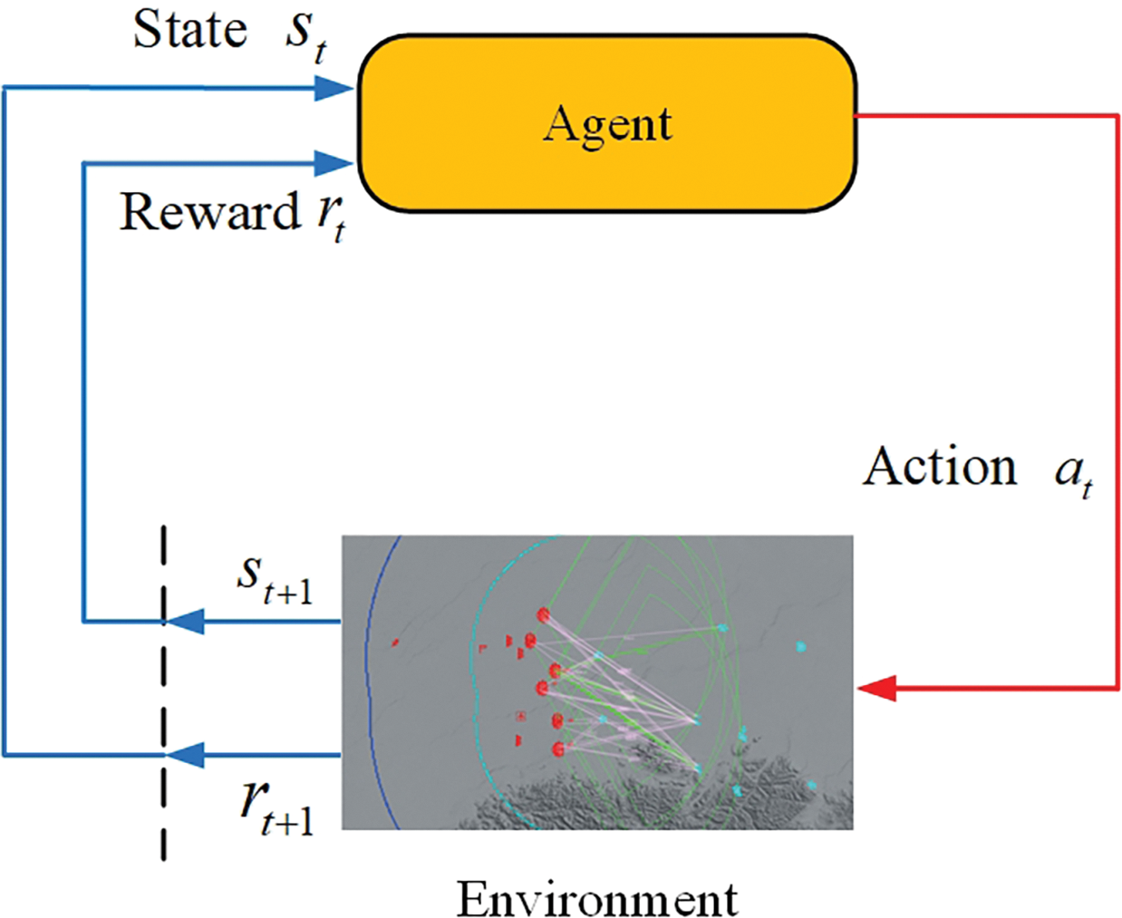
Figure 2: Single-agent architecture

In the process of multi-agent training, the strategy of each agent is changing, so from the perspective of each agent, the environment becomes very unstable, and the actions of other agents bring about environmental changes.

In this paper, each red combat unit is modeled as a decision-making agent. The agent obtains its current state oi from the current environmental state, outputs actions ai after making decisions, and forms a joint action with the actions of other agents, which is input into the environment. After the environment executes the action, it updates its state and feeds back a joint reward to each agent.

2.2 Markov Decision Process

The RL task satisfying the Markov property is called the Markov decision process (MDP). MDP is a mathematical model of sequential decision-making, which is mainly suitable for systems with Markov properties to simulate the stochastic strategies and returns of agents. RL generally uses MDP to model the problem. MDP is represented by five tuples ⟨S,A,P,R,γ⟩, where S is the set of states of the intelligence, A is the set of actions of the intelligence, P is the state transfer function, R is the set of reward, and γ is the discount factor [23]. At moment t, given a state s and action a, the next state s′ and the reward r can be represented by p:

p(s′,r|s,a)=Pr{st+1=s′,rt+1=r|st=s,at=a}(1)

The expected reward for the state-action is:

r(s,a)=E[rt+1|st=s,at=a]=∑r∈Rr∑s′∈Sp(s′,r|s,a)(2)

State transition probability:

p(s′|s,a)=Pr{st+1=s′|st=s,at=a}=∑r∈Rp(s′,r|s,a)(3)

The expected reward for the state-action-next state:

r(s,a,s′)=E[rt+1|st=s,at=a,st+1=s′]=∑r∈Rrp(s′,r|s,a)p(s′|s,a)(4)

The ultimate goal of RL is to find an optimal strategy π∗ to maximize the expected return:

π∗=arg maxπE[R|π](5)

2.3 Partially Observable Markov Decision Process

The MDP model is used to describe a situation in which there is only one agent in the environment, and it cannot explain the interaction problem of multiple agents well. The important premise of the MDP model is that agents can completely observe the environment. That is, they can obtain environmental information completely and accurately. However, in the actual complex environment, because the environment is full of a lot of noise and interference, each agent can only get a small part of the state of the environment, so a model closer to the environment is needed, that is, the POMDP, which can be regarded as the expansion of Markov decision-making process and is still based on the similar assumption of MDP.

In POMDP, each agent can only make synchronous decisions independently according to the information it can obtain. It is hoped that a strategy network that can make independent distributed decisions can be trained for each combat unit by using multi-agent RL technology, and the agent strategies obtained from these strategy networks can achieve a certain degree of self-cooperation.

POMDP is represented by seven tuples ⟨S,A,P,R,O,Z,γ⟩: S is the system state set, that is, the joint state of multi-agents, S=(s1,s2,⋯,sN); A=(a1,a2,⋯,aN) is the action set of multi-agent; P is the state transition function, P:S×a1×⋯×aN×S→[0,1], according to the current state of the system and the joint action of the agent, the probability distribution of the next state of the system is given; R is a reward in return, R=(r1,r2,⋯,rN); O is an observation set of a group of agents on the environment, in POMDP, the result depends on the potential environmental state; Z is the observation function, Z:S×A→Δ(O), which reflects the relationship between the multi-agent system and the observed value; γ is the discount factor, which describes the influence of future rewards on the reward function of agents. It reflects the uncertainty of future rewards and ensures that the reward function is bounded.

As shown in Fig. 3, by introducing the belief state function, the POMDP problem is transformed into a Markov chain based on the state of belief space to solve, that is, to solve the belief state function and strategy problem. Belief MDP is usually described as a quadruple ⟨B,A,Pb,rb⟩, where B=Δ(S), represents a series of state spaces; A is the action space; D, Pb:B×A→B, belief transfer function; rb(b,a)=∑s∈Sb(s)r(s,a) is the reward function. Therefore, under Belief MDP, the value function is:

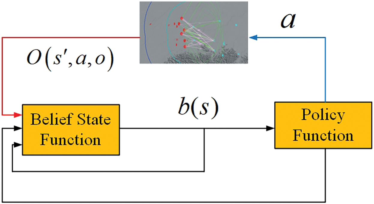
Figure 3: POMDP

Vt+1(b)=maxa∈A⁡[rb(b,a)+γ∑b′∈BPb(b,a,b′)Vt(b′)]=maxa∈A⁡[∑s∈Sb(s)r(s,a)+γ∑o∈OPr(o|a,b)Vt(boa)](6)

πt+1(b)=arg maxa∈A[∑s∈Sb(s)r(s,a)+γ∑o∈OPr(o|a,b)Vt(boa)](7)

3  Algorithm Description

3.1 MADDPG Algorithm

Fig. 4 is a schematic diagram of MADDPG algorithm training based on the actor-critic framework. Each agent has four networks: Actor network, Critical network, Target Actor network, and Target Critic network. MADDPG algorithm adopts the training mode of “centralized training and decentralized execution”.

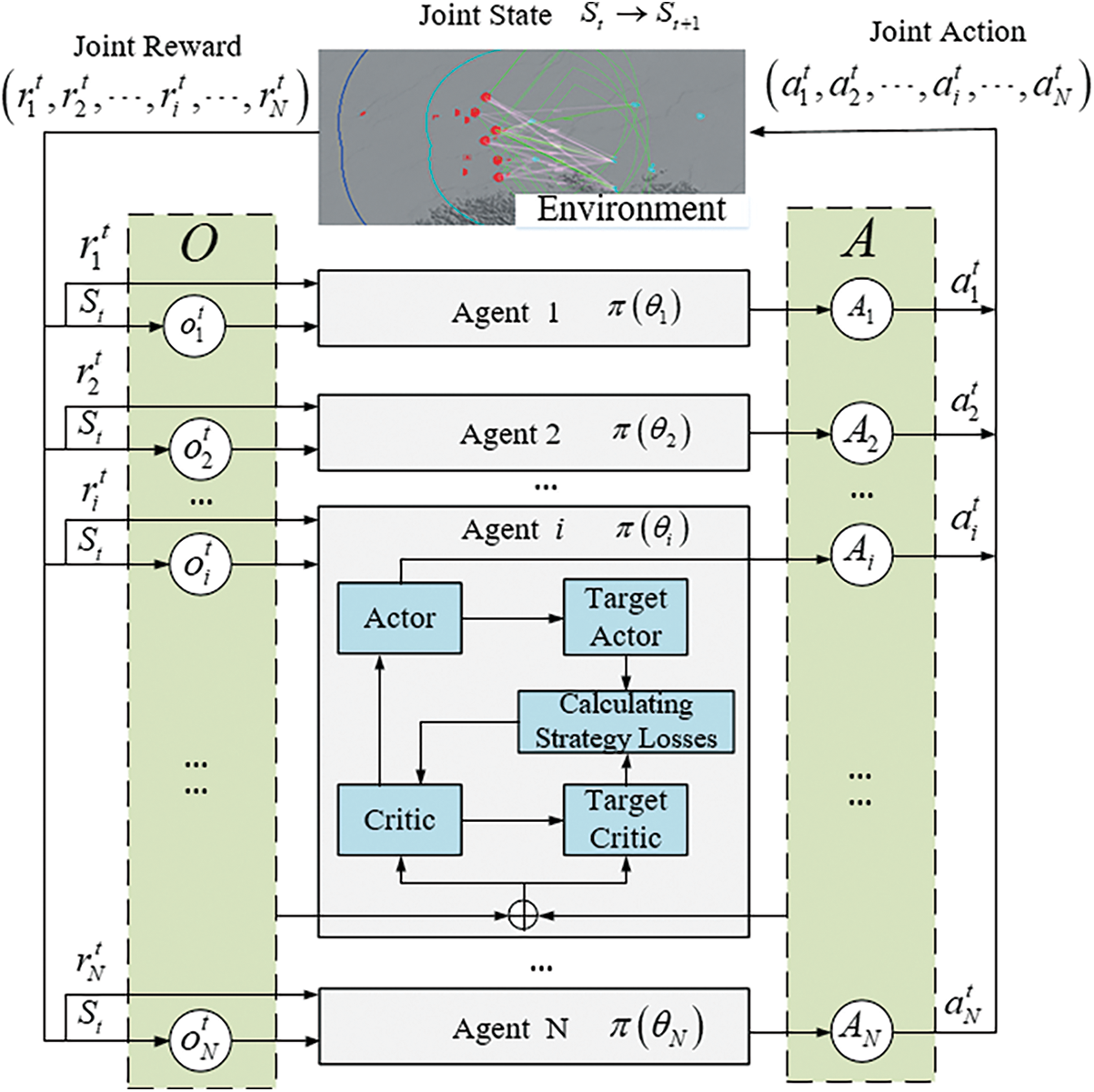
Figure 4: Schematic diagram of MADDPG algorithm

Using the above framework, additional information can be used to assist network training in the model training stage, but no additional information is used in the model execution stage. During training, the central controller can obtain the action, state observation, and reward value of each executive agent, and use n critic networks to evaluate the decision-making quality of n strategic networks. After the training, the central controller is no longer used to evaluate the quality of the decision, and only the strategy network of each executive agent produces the decision.

Assuming that there are N agents in the environment, and the joint strategy space of agents is π=(π(θ1),π(θ2),⋯,π(θN)), where θ=(θ1,θ2,⋯,θN) is the set of strategy parameters, the action of agent i under observation oi is πi(ai|oi), and the gradient of the agent i is:

∇θiJ(θi)=Es∼pμ,ai∼πi[∇θilog⁡πi(ai|oi)Qiπ(x,a1,a2,⋯,aN)](8)

Qiπ(x,a1,a2,⋯,aN) is the central evaluation function; x is environmental information, x=(o1,o2,⋯,oN).

Change the random strategy into deterministic strategy, and μθi (abbreviated as μi) represents the strategy of the agent i, then Eq. (8) is rewritten as:

∇θiJ(μi)=Es,a∼D[∇θiμi(ai|oi)Qiμ(x,a1,a2,⋯,aN)|ai=μi(oi)](9)

The training of the Critic function can be updated by minimizing the loss function:

L(θi)=Ex,a,,r,x′[(Qiμ(x,a1,a2,⋯,aN)−y)2](10)

y=ri+γQi′(xi,a1′,a2′,⋯,aN′)|aj′=uj′(oj)(11)

where μ′={μθ1′,⋯,μθN′} is the action function of the target network, corresponding to the action function parameter θi′ in the target network i, Qi′ is the evaluation function in the target network i.

In MADDPG algorithm, the execution actions of each agent are known, and even if the strategy changes, the environment is relatively stable, because:

p(s′|s,a1,a2,⋯,aN,π1,π2,⋯,πN)=p(s′|s,a1,a2,⋯,aN)=p(s′|s,a1,a2,⋯,aN,π1′,π2′,⋯,πN′)(12)

As long as the actions ai generated by πi′ and πi are consistent, p(s′|s,a1,a2,⋯,aN) will not change, and the whole environment is relatively stable.

3.2 MADDPG-D2 Algorithm

3.2.1 Dual Experience Pool Mechanism

The experience playback mechanism can eliminate the correlation between data while ensuring the full utilization of the data. While the traditional experience playback method cannot efficiently utilize the experience samples that have positive significance for network training, the priority-based experience playback method accelerates the learning process of the network by searching for experience samples with high importance, but the training efficiency of the algorithm is low because it needs to frequently perform the operations of prioritizing and updating, which increases the algorithm’s training cost.

Distinguishing from the above methods, the dual experience pool mechanism considers using two experience playback pools A and B for categorizing and storing experiences of different qualities according to their different degrees of importance. In the training phase of the network model, only experience samples are proportionally selected from different experience buffer pools. The sampling ratio is adjusted upward in the experience buffer pools with a higher degree of importance. In contrast, a small number of experience samples with a low degree of importance are selected in each batch in order to ensure the diversity of the samples, and the distribution of sampled experience states is changed by the adjustable size of the experience pools and the ratio of sampled experiences, which improves the quality of the training of the network model and accelerates the convergence speed. The dual experience pool mechanism has the same time complexity as the ordinary experience playback method and does not increase the space complexity.

How to judge the quality of this group of data, an important criterion is the deviation of temporal difference (TD) δ, that is:

δ=(y−Qπ(s,a1,a2,⋯,aN))2(13)

δ is greater, which means that the difference between the evaluation value and the actual value of the target network is greater. For agent training, the higher the quality, the more it is necessary to increase the sampling frequency, update the values of the target network and the evaluation network, and accelerate the satisfactory training effect.

For a sample experience, entering the experience replay pools A or B is mainly determined by its own δ and the average value δ¯ in the replay pool. Firstly, the network model is initialized, and the initial average value δ¯ in two experience replay pools is set to 0; When an agent interacts with the environment to generate a piece of empirical sample data, δ of the sample data is calculated, and the average value δ¯ of all empirical samples in the empirical replay pool is updated at the same time. δ is compared with the average value δ¯, and if it is greater than the average value δ¯, the sample data is stored in the empirical replay pool A. Otherwise, it is stored in the empirical replay pool B. In this way, data experiences are categorized according to importance before storage, reducing the operations of assigning and updating priorities. During sampling, experience groups are drawn proportionally from different experience playback pools. The dual experience pool mechanism works as shown in Fig. 5.

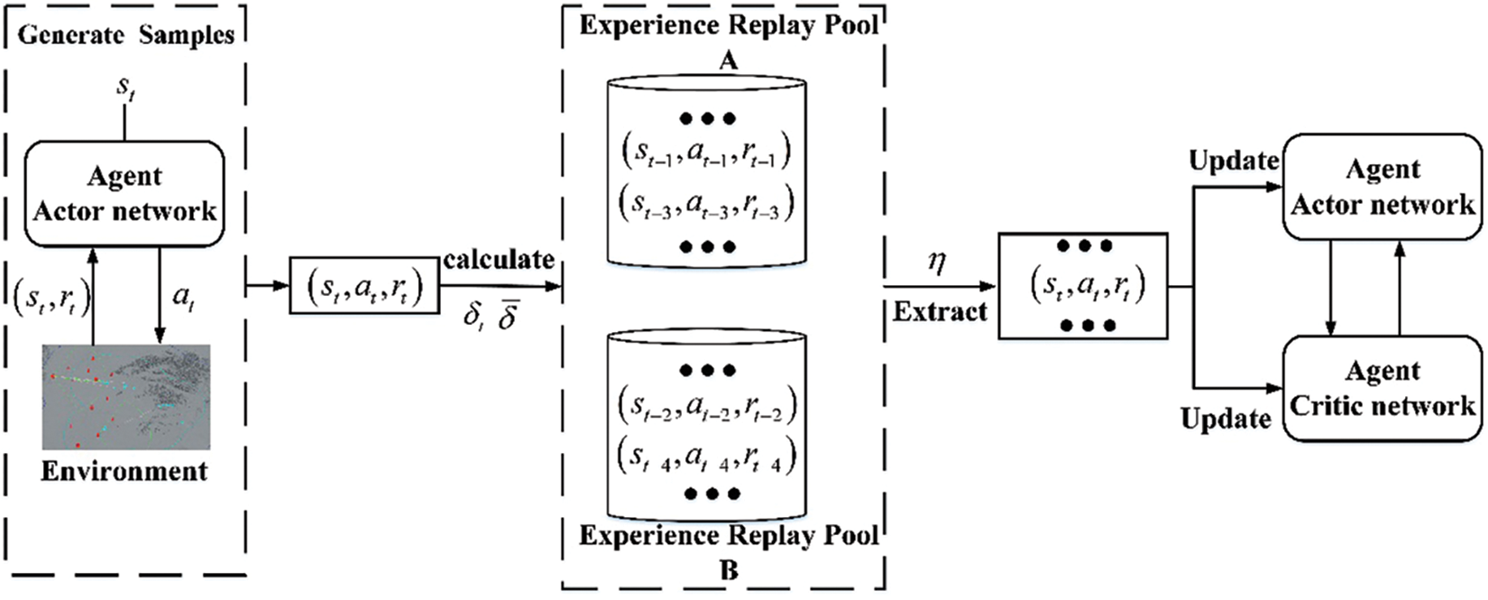
Figure 5: Dual experience pool mechanism

3.2.2 Dual Noise Mechanism

In the MADDPG algorithm, the actions executed by the agent’s strategy are unique, which may lead to insufficient exploration of the environment by the agent, and thus additional exploration of the noise is needed to obtain an experience sample that is more useful to the agent. A common approach to improve the exploration capability of an agent is to add noise to the action space of the agent. In the algorithm based on Actor-Critic architecture, the Actor network is used to predict the strategy of the agent, so to better explore the complete action state space and to improve the exploration ability, this paper introduces random noise in the Actor network, which changes the decision-making process of the action into a stochastic process, and then samples the values of the action from this stochastic process. The Ornstein-Uhlenbeck (OU) process has a good correlation in time sequence, which can make the agent explore the environment with momentum properties, but this exploration strategy is not the final action strategy. It is only used in the training process to generate the actions given down to the environment, so as to obtain the relevant data, which is used to train the intelligent body to obtain the optimal strategy.

The differential form of OU random noise Nt is

dNt=θ(μ−Nt)dt+δdBt(14)

where μ is the mean value; θ is the speed at which the noise tends to average; δ is the fluctuation degree of noise; Bt is the standard Brownian motion.

At the same time, to increase more randomness in the learning process of agents, increase the coverage of learning, and obtain higher quality training data, random Gaussian white noise with mean 0 and variance σ2 is added to the action space. Applying Gaussian noise to action exploration can help agents explore more of the action space and discover new strategies and beneficial behaviors. In a Gaussian white noise distribution, most of the noise values are concentrated near the mean 0, while noise values further away from the mean have a lower probability of appearing. The variance determines the distribution range of the Gaussian noise, the larger the variance of the Gaussian noise, the wider the distribution range of the noise values, and the larger the exploration range of the agent.

f(x|0,σ2)=1σ2πe−x22σ2(15)

where the variance σ2 is used to measure the exploration intensity of the agent, the strategy π(st) generated by the agent through the strategy network is also correlated with the Gaussian white noise in state st. A Gaussian noise of 0 ensures that while the optimal action can be executed, actions that differ from the optimal action also have a certain chance of being executed.

The dual noise working mechanism of OU random noise and Gaussian noise is shown in Fig. 6.

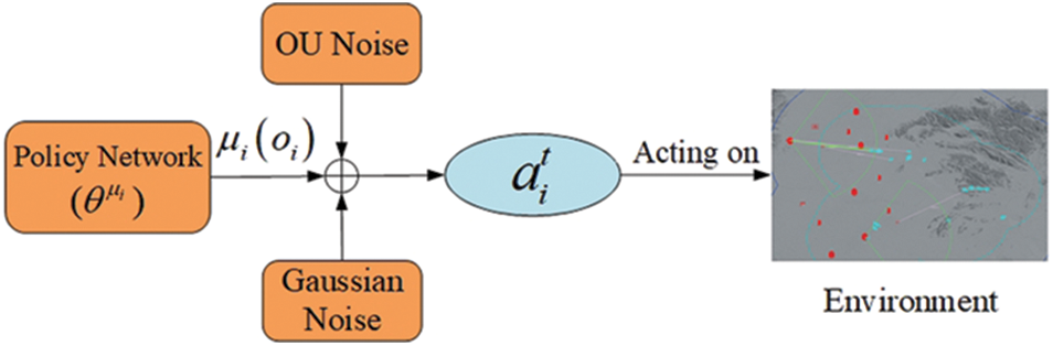
Figure 6: Dual noise mechanism

As an example, the block diagram of the MADDPG-D2 algorithm for the agent i in the MADDPG-D2 algorithm is shown in Fig. 7.

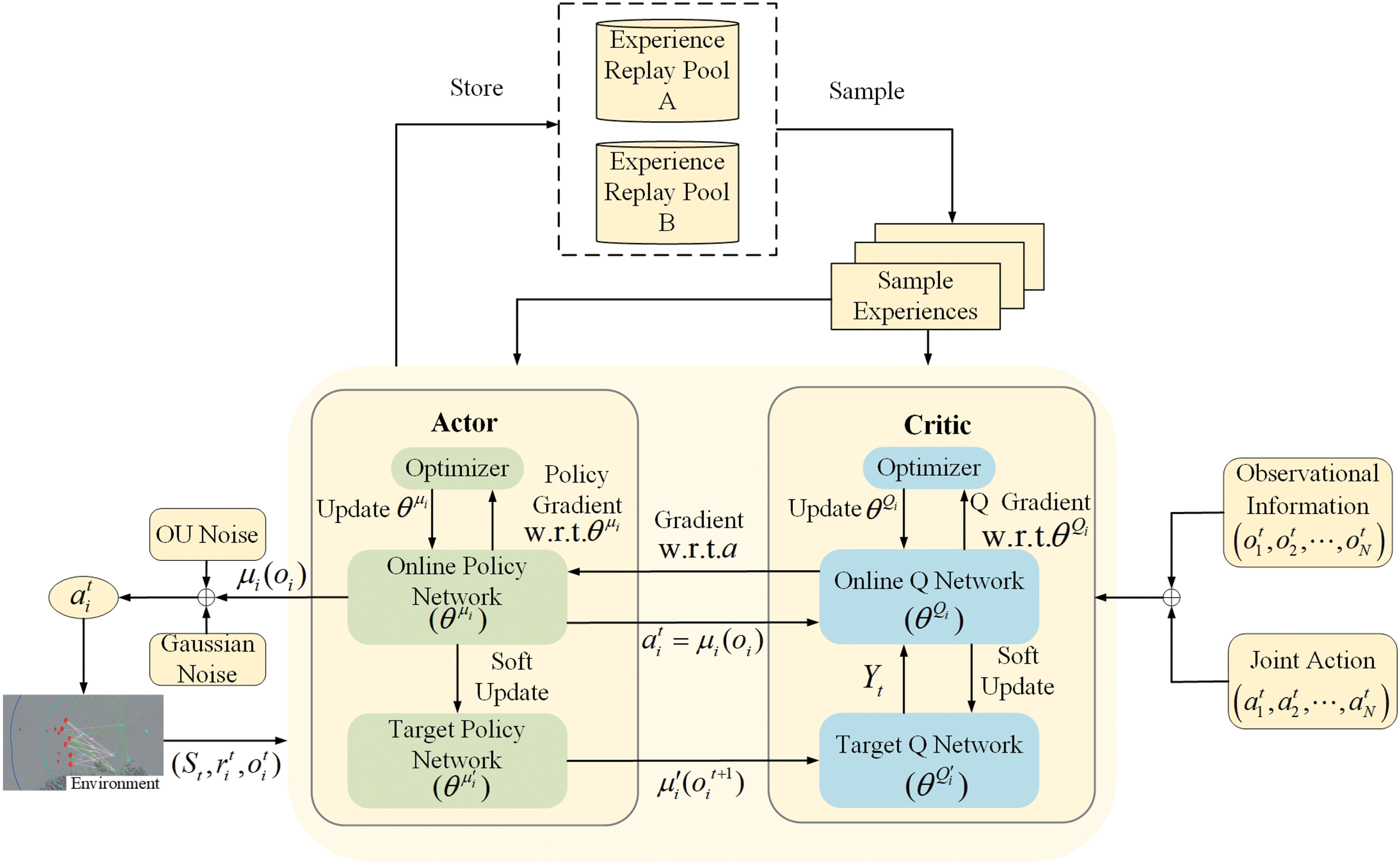
Figure 7: Schematic diagram of MADDPG-D2 algorithm for agent i

3.3 Integration of Prior Knowledge

This section mainly constructs the empirical data of domain experts. In this paper, an expert sample experience pool is constructed, and the domain expert experience data is transformed into the corresponding state-action sequence and stored in the expert sample experience pool. In the pre-training stage, the optimal strategy of the agent is the strategy output from the knowledge rule base, that is, prior knowledge. Based on the network decoupling training framework, the agent extracts a small number of samples from the expert sample experience pool and passes them into the MADDPG-D2 algorithm for action selection. Generate training data by interacting with the environment and store the data in the experience pool for knowledge updates. The experience pool is divided into some memory spaces, the size of the memory space is set, and the allocated array data is passed in and stored in turn. When the storage space is larger than the memory space, the previous data is eliminated, and at the same time, the batch-size data is continuously extracted and transmitted to the learning module to update the strategy network, thus reducing the loss function. By using prior knowledge to pre-train the parameters of the MADDPG-D2 network, a good initial policy for multiple agents can be provided, which can significantly reduce the exploration and training time, and reduce the probability of intelligence falling into locally optimal solutions.

The prior knowledge used in this paper mainly includes aspects such as existing rule guidelines for RTA, domain expert knowledge and scenario elements to prioritize the various types of units that may appear, and eventually form a set of prioritized experiences, pre-training the network, which mainly consists of the following parts:

(1)   Strike incoming targets according to the degree of importance, which must ensure the elimination of the most important incoming targets, with the highest priority being given to the blue fighters.

(2)   Maximize the performance of the interception systems used to ensure that they are compatible with the parameters of the incoming target and maximize interdict efficiency.

(3)   If the conditions for interception are met, long-range units should first intercept blue’s jamming aircraft located in the patrol area.

(4)   The depth of the kill zone of interception systems should be utilized to implement the maximum number of interceptions.

(5)   If conditions permit, more than two of our units should be utilized to conduct concentrated interception on the incoming target to guarantee the reliability of the interception and to increase the probability of destruction of important targets.

(6)   Based on the feedback information of each intercepting unit after the execution of the mission, the allocation strategy should be rationally adjusted and the next round of decision-making should be prepared.

(7)   Based on their own status, each interception unit determines the sector (altitude) for intercepting the incoming target.

In the above way, the incorporation of prior knowledge and experience replay is achieved to improve the training effect of the MADDPG-D2 algorithm. The specific process is shown in the following Fig. 8.

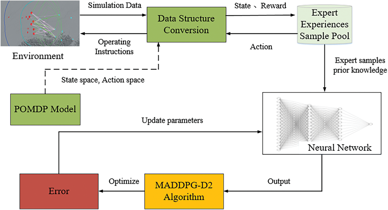
Figure 8: Pre-training process

At this time, the goal of training is changed from finding a strategy with the highest cumulative reward value to finding a strategy closest to the expert strategy [24]. The essence of this training method is to find a strategy with the smallest difference in value function between the strategy and the expert strategy.

minπ[V(πE)−V(π)](16)

where V(πE) is the value function of the expert strategy and V(π) is the value function of the strategy learned by the agent.

To make the agent learn the expert strategy stably, this paper adds the calculation of behavior clone loss value [25].

LBC=∑i=1(Si,G(i))‖π(si|θπ)−ai‖2(17)

where LBC is the loss of behavior cloning, (Si,G(i)) is the sample set, π(si|θπ) is the strategy learned by the agent, θπ is the network parameter of the agent, and ai is the action in the sample set in the corresponding state si. By calculating LBC, the action difference between the two strategies is minimized, and the strategy finally learned by the agent is as similar as possible to the expert strategy.

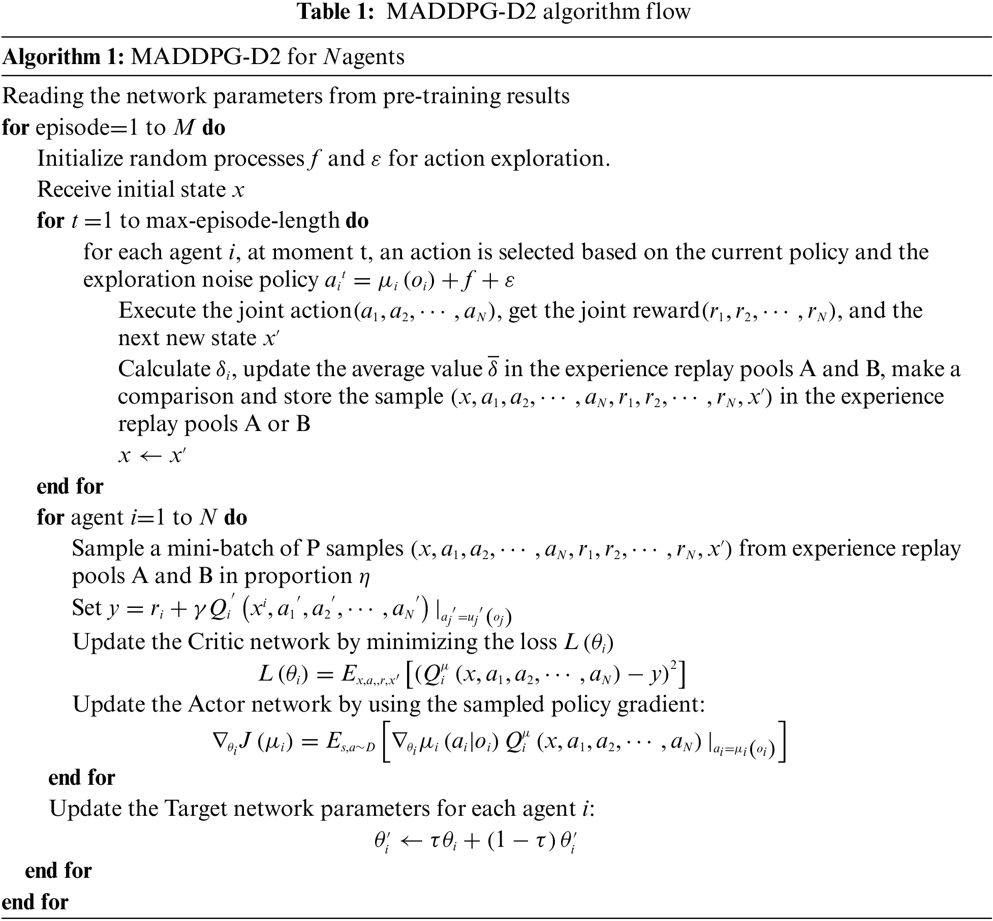
The pseudo-code of the MADDPG-D2 algorithm is shown in Table 1.

However, the improved MADDPG-D2 algorithm also has some defects:

1)   Since the MADDPG-D2 algorithm adopts the “centralized training, distributed execution” mode of operation, each Critic network needs to observe the states and actions of all the agents. When the number of agents is very large, the state space is too huge, which makes the solution difficult.

2)   Each agent corresponds to an Actor and a Critic network. When the number of agents is large, there are a large number of models which require high computational power.

4  POMDP Model

4.1 State Space

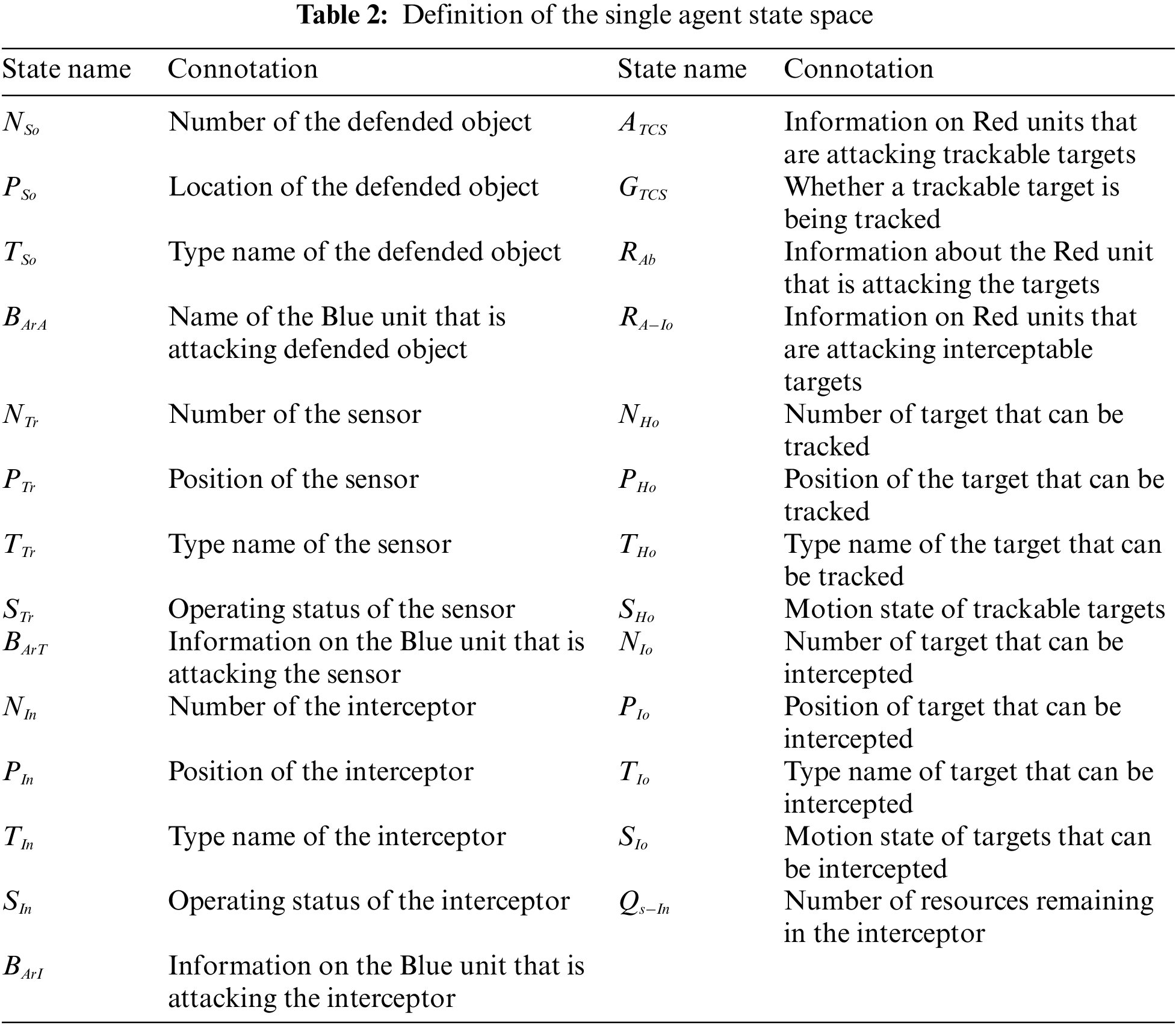
In the MAS, due to the increase of combat entities, it brings more action and state space. For a single red agent, there are four state spaces, and the states of all red agents constitute the overall red state:

1) Observable state information of the protected object; 2) the state of its own unit, including resource allocation, sensor, and interceptor state, and the target state information of the attacker within the interception range of the unit; 3) observable state information of incoming targets; 4) observable state information of enemy units that can be attacked. The definition of agent state space is shown in Table 2.

4.2 Action Space

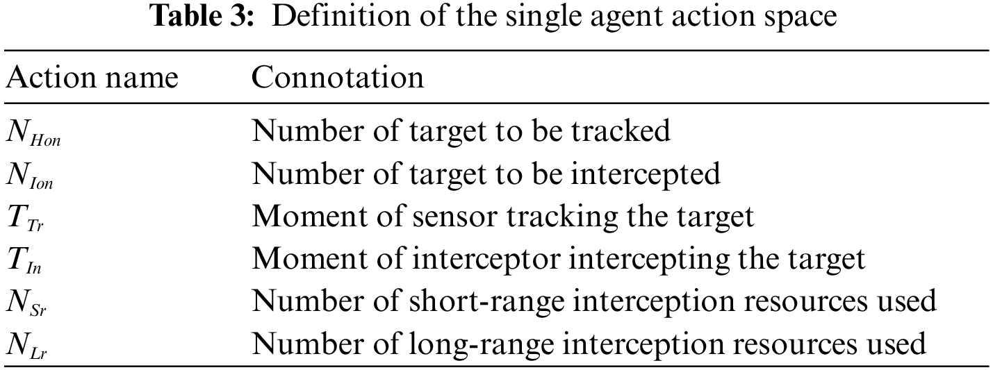
For the red single agent, the output of the action by the agent includes 1) the number of the incoming targets to be tracked; 2) the number of incoming targets to be intercepted; 3) the timing when the sensor tracks the target; 4) the timing of intercepting the target; 5) the number of resources used to intercept the target. The definition of action space is shown in Table 3. The action space of all red agents constitutes the whole redaction space.

4.3 Reward Function

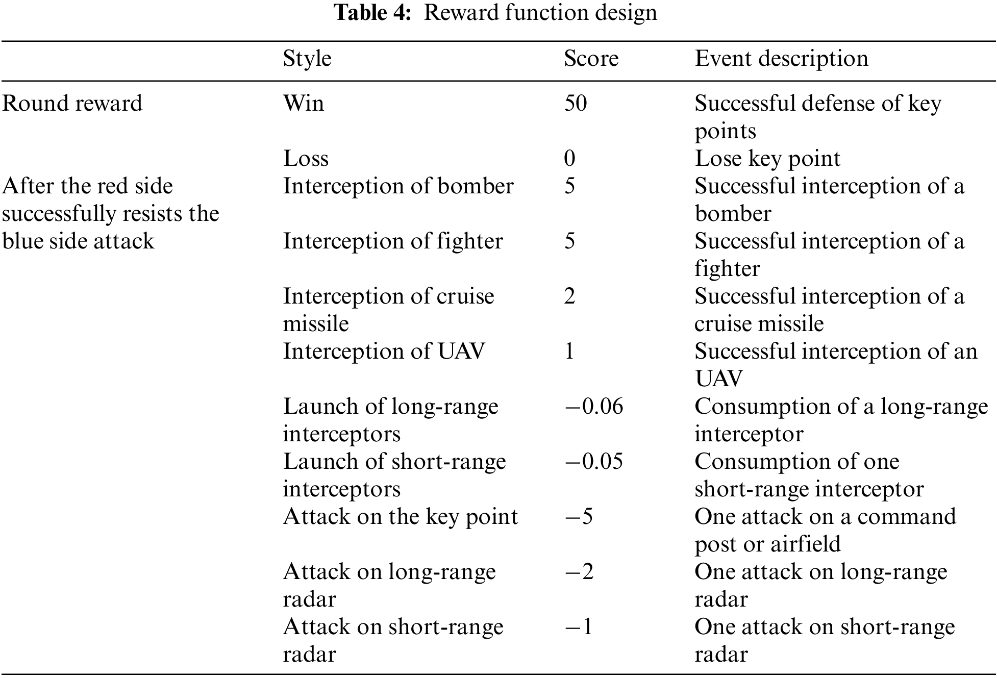
The training process of DRL is essentially a process in which the agent interacts with the environment, gets feedback after the interaction, and adjusts the action according to the feedback to gradually maximize the reward. In this process, the learning of the action is mainly guided by the reward function, so it is necessary to reasonably design the reward function, the design of the reward function will directly affect the training effect of the model and the training efficiency.

In the MADDPG-D2 algorithm, each agent can design its reward function separately. A good reward function can accelerate the learning speed of agents and make the algorithm converge faster. The setting of the reward function should not be too sparse, so it is difficult for agents to trigger the “reward mechanism” and roam for a long time, that is the “plateau problem”. In the above-mentioned combat scenario, the goal is that all red units complete the task of intercepting the blue attack target and ensuring their safety, so the task is a cooperative task, and all decision-making agents share a global reward value.

To better coordinate the reward function and reward the agent at the right time, the task-based reward mechanism is introduced: after the red side has completed a wave of attacks by the blue side, it will be given a larger reward. At the same time, after the red side intercepted the important high-value targets of the blue side, it was given certain rewards.

Where Ci stands for the target type of blue side, including bombers, UAV, cruise missiles and fighters; ni stands for the number of targets i intercepted by the blue side. The reward function design is shown in Table 4.

f={∑i=1K⁡niCi+50,Win∑i=1K⁡niCi, Loss(18)

5  Simulation Environment and Troop Setting

5.1 Simulation Environment and Parameter Setting

The simulation environment used in this paper is shown in Fig. 9. The training hardware used for the experiments includes Intel Xeon E5-4655V4 CPU with eight cores, 512 GB RAM, and RTX3060 GPU with 12 GB video memory.

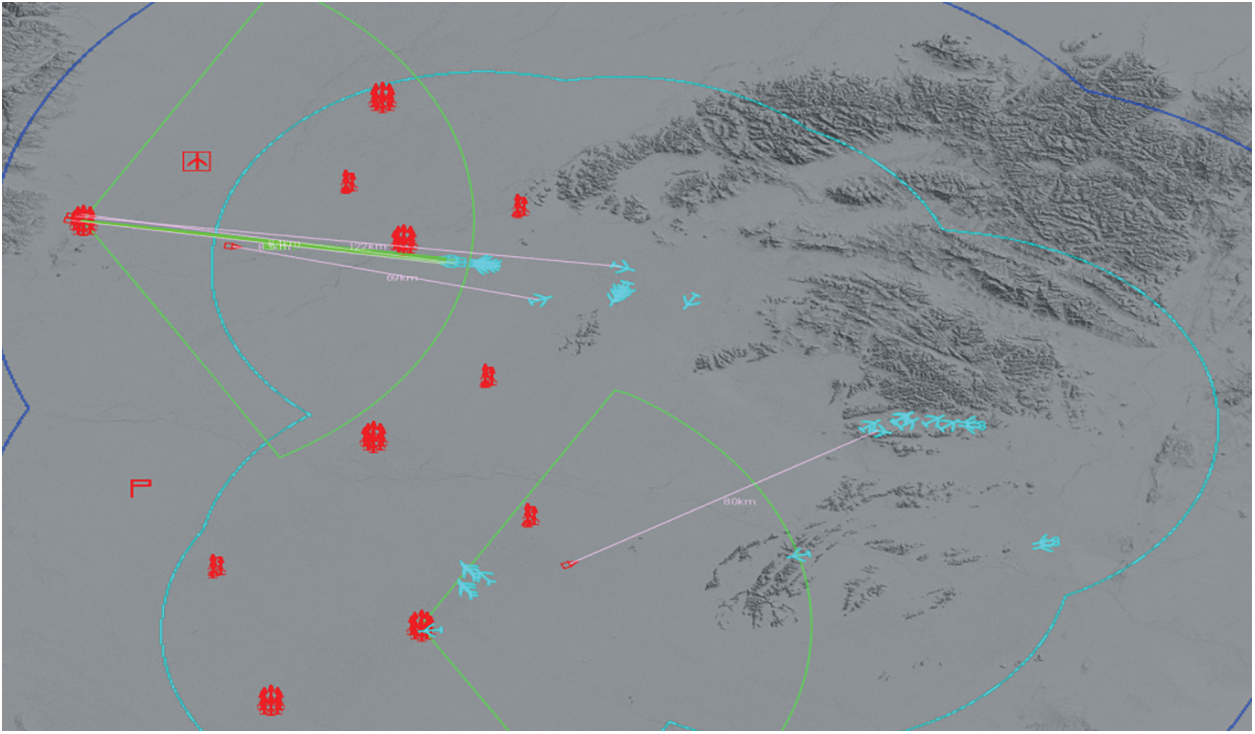
Figure 9: Simulation environment

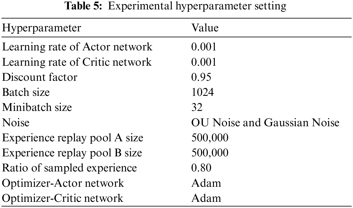
Several sets of orthogonal tests are conducted prior to the formal experiment, and the experimental hyperparameter settings are shown in Table 5.

5.2 Troop Setting

In the simulation experiment, the main objective of the red side is to defend the key points from being destroyed, i.e., to protect the important facilities of the red side (1 command post and 1 airfield), and at the same time to destroy as many incoming targets of the blue side as possible while preserving itself; the main task of the blue side is to attack the airfields and command posts of the red side, and at the same time to destroy the exposed red side’s defense weapons and positions. The Red and Blue forces are set up as shown in the Table 6.

5.3 Training Process

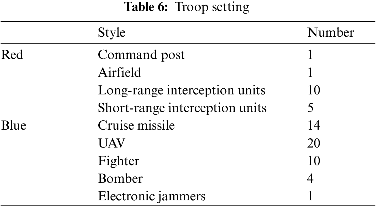
Fig. 10 shows the flowchart of training using the MADDPG-D2 algorithm. The flowchart is divided into three parts: pre-training, sampling and training. In the pre-training stage, the parameters of the multi-agent network are pre-trained using the prior knowledge, which can provide a good initial strategy for the multi-agent body, and at the same time greatly reduce the exploration and training time; after the pre-training is completed, the multi-agent body interacts with the environment for sampling, which requires converting the data output from the environment into state information and reward functions according to the state space, action space and reward function in the POMDP model; the data output from the environment is converted into state information and reward values, and convert the actions output from the neural network into combat commands, generating a large number of data samples; during training, the data samples generated by interaction are used to input into the MADDPG-D2 algorithm, which updates the network parameters by calculating the error between the samples and the neural network outputs, continuously optimizes the strategies of the multi-intelligent bodies, and finally finds the strategy with the highest cumulative reward value.

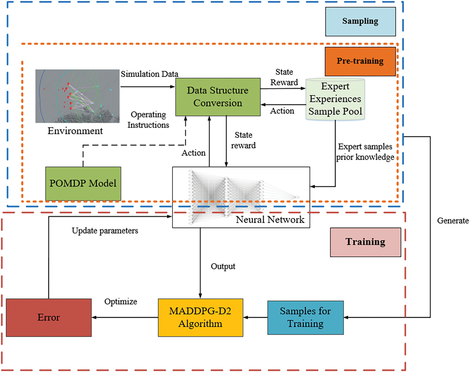
Figure 10: Training process

6  Experimental Results and Analysis

6.1 Comparison of Agent Architecture

This section compares the average win rate and average reward of the Deep Deterministic Policy Gradient (DDPG) algorithm under single-agent architecture and the MADDPG-D2 algorithm under multi-agent architecture, and also comparatively analyzes the performance of the RULE algorithm.

Fig. 11 shows the comparison of the average win rate of agents under the two architectures. The abscissa is the number of training rounds, the total coordinate is the win rate, and the shaded part is the error zone. Analysis shows that the initial winning rate of the MADDPG-D2 algorithm trained with the prior knowledge can reach about 10%, which is higher than that of the untrained DDPG algorithm, and slightly lower than that of the RULE algorithm, indicating that the agents trained with the prior knowledge can master certain principles of task allocation and rules of firepower utilization. And the difference in the initial winning rate of the MADDPG-D2 algorithm and that of the RULE algorithm is not very large, indicating that the a priori knowledge is more successfully applied to the pre-training of the MADDPG-D2 algorithm. By comparison, when the training reaches 50,000 rounds, the win rate of the DDPG algorithm under single-agent architecture can reach 41.73%, while the win rate of agents trained by multi-agent architecture can reach 69.15%, which is 46.72% higher than the former, which shows that it is reasonable to use multi-agent architecture when dealing with large-scale DTA problem, and the win rate of red agent can be effectively improved by using MADDPG-D2 algorithm. Before the first 20,000 rounds, the win rate of single-agent architecture is higher than that of multi-agent architecture, but after 20,000 rounds, the win rate of single-agent architecture does not improve obviously, which may be because after 20,000 rounds, multi-agents cooperate, master the rules of firepower application and certain tactical tactics, and can better deal with large-scale blue attack targets, and the corresponding emerging behavior will be carried out in the following chapters.

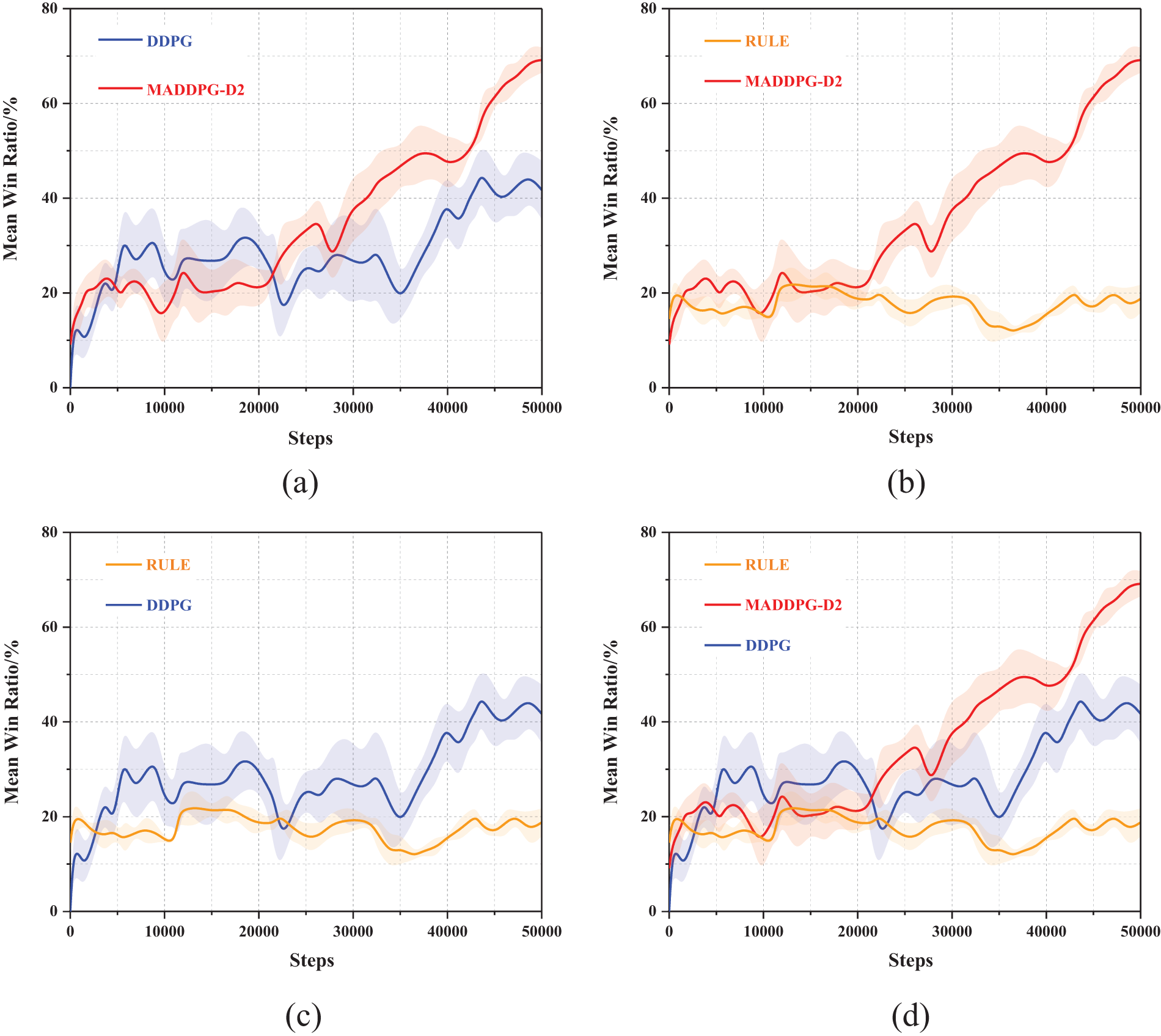
Figure 11: The average win rate curve under different architectures. (a) DDPG and MADDPG-D2; (b) MADDPG-D2 and RULE; (c) RULE and DDPG; (d) MADDPG-D2, RULE and DDPG

At the same time, it can be found that the RULE algorithm has already specified and solidified the shooting timing and conditions, so the RULE agent plays more stable, the win rate is stable at about 20%, and there is no big fluctuation, while the MADDPG-D2 algorithm, which integrates the prior knowledge, can reach a high level, and there is a certain degree of improvement in the win rate, which shows that the method trained by intelligent algorithm is effective.

Fig. 12 shows the average reward scores of three algorithms when the training rounds are 25,000 and 50,000. When the training round is 25,000, the MADDPG-D2 algorithm can get a bigger reward, followed by the DDPG algorithm, and the average reward value of the RULE algorithm is the smallest. The analysis may be because when the training round reaches 25,000, the MADDPG-D2 algorithm has a higher win rate, and there is a greater probability of winning 50 points at the end of each round. At the same time, combined with the analysis of countermeasure loss data in the next section, the MADDPG-D2 algorithm has learned some strategies at this time, which can intercept more high-value targets such as fighters, so the average reward is higher; after a certain number of rounds of training, the average reward of the MADDPG-D2 algorithm and the DDPG algorithm has been improved to a certain extent. When the number of training rounds reaches 50,000, the average reward value of the MADDPG-D2 algorithm can reach 125.96, with a variance of 6.4, while that of the DDPG algorithm and the RULE algorithm is 81.97 and 36.43, with a variance of 8.9 and 3.6, respectively. Therefore, the intelligent algorithm can get a higher reward value, and it is more effective to adopt a multi-agent architecture and solve it through a multi-agent algorithm when dealing with large-scale DTA problem.

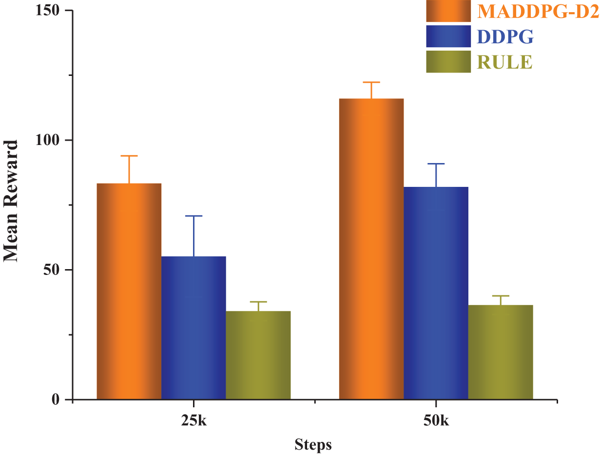
Figure 12: Average reward under different architectures

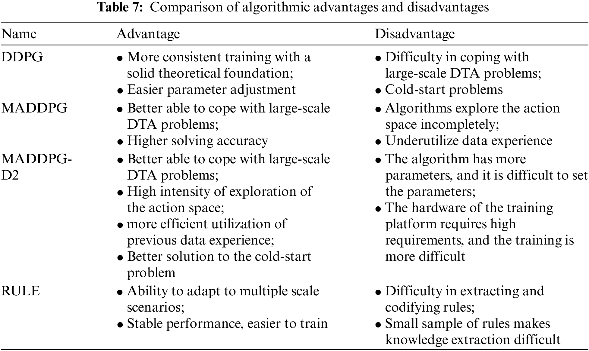
According to the above experimental results and theoretical analysis, the advantages and disadvantages of the three algorithms are shown in Table 7.

6.2 Combat Loss and Adversarial Data Analysis

This section analyzes the performance of the DDPG algorithm under single-agent architecture, the MADDPG-D2 algorithm under multi-agent architecture, and the RULE algorithm in the training process. This section selects the battle losses of the red and blue sides when the training rounds are 25000 and 50000.

As can be seen from Table 8, after training, the performance of the agents using MADDPG-D2 and DDPG algorithms has been improved to some extent. Horizontally, the number of long-range radar losses, the number of close-range radar losses, and the number of attacks on key points have all decreased to a certain extent, indicating that the agents learn some strategies after training, and can preserve themselves better and reduce the number of attacks on themselves, while the RULE algorithm agent play more stably, and are almost unaffected by the number of training rounds, it is because the RULE algorithm is more fixed, the radar start-up time, the allocation time, the number of intercepted munitions all have standard specifications, and are not affected by training, but its win rate is lower. In comparison, the performance of the MADDPG-D2 algorithm is better than the DDPG algorithm, mainly because the MADDPG-D2 algorithm adopts multi-agent architecture, multi-intelligent bodies cooperate, and the advantages are complementary to each other, and in the face of the large-scale blue target incoming attacks, the multi-agent architecture is more appropriate. Analyzing the number of attacks on the key points, it can be seen that the trained agents by intelligent algorithm can effectively reduce the number of attacks. In the training rounds of 25,000, the number of attacks on the key points using the MADDPG-D2 algorithm and the DDPG algorithm are 2.643 and 4.924, respectively; while in the training rounds of 50,000, the number of attacks are 1.681 and 3.025, the number of attacks have decreased significantly, indicating that the agents have learned certain defensive strategies. From the detailed analysis of the subsequent interception, it can be seen that to defend the important place from being attacked, the red side will even choose to sacrifice a small number of fire units to attract the blue side’s firepower to achieve the purpose of preserving the important place of the red side.

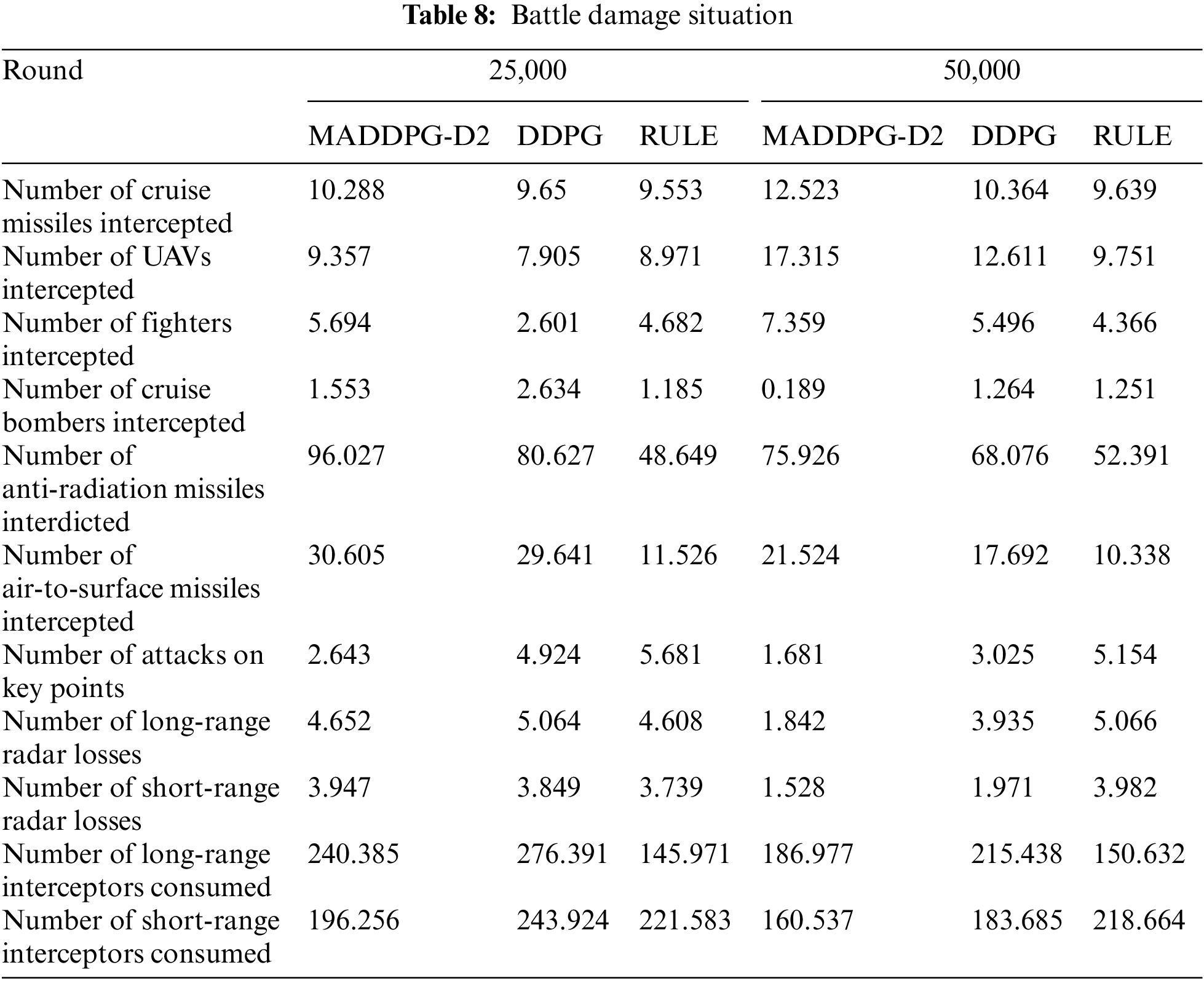
According to the consumption of long-range interceptor, at 25,000 rounds, the loss of the MADDPG-D2 algorithm is 240.385, and that of the DDPG algorithm is 276.391. After 50,000 rounds of training, the loss of the MADDPG-D2 algorithm is 186.977, and that of the DDPG algorithm is 215.438, which decreased by 22.22% and 22.05% respectively. Compared with the consumption of long-range interceptor, the consumption of the MADDPG-D2 algorithm is lower than that of the DDPG algorithm, which shows that the MADDPG-D2 algorithm can consume fewer interception resources, reduce the number of attacks, and have a higher interception rate. The remote radar using the RULE algorithm has more losses, reaching 5.066 when the number of training rounds is 50,000. This is mainly because the RULE algorithm intercepts the targets entering the kill zone in sequence, the detection and killing range of the long-range firepower unit is larger than that of the short-range firepower unit, and the long-range radar is turned on prematurely, exposing its position and being destroyed by the blue incoming targets.

6.3 Ablation Experiment

To study the effect of the two mechanisms on the training effect, this paper designs ablation experiments to compare the difference in effect by adding or subtracting two mechanisms to the MADDPG algorithm with a total of four different algorithm setups. The experimental settings are shown in Table 9.

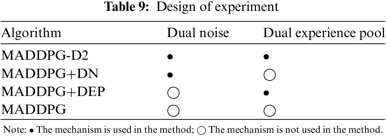
The results of the ablation experiment are shown in Fig. 13.

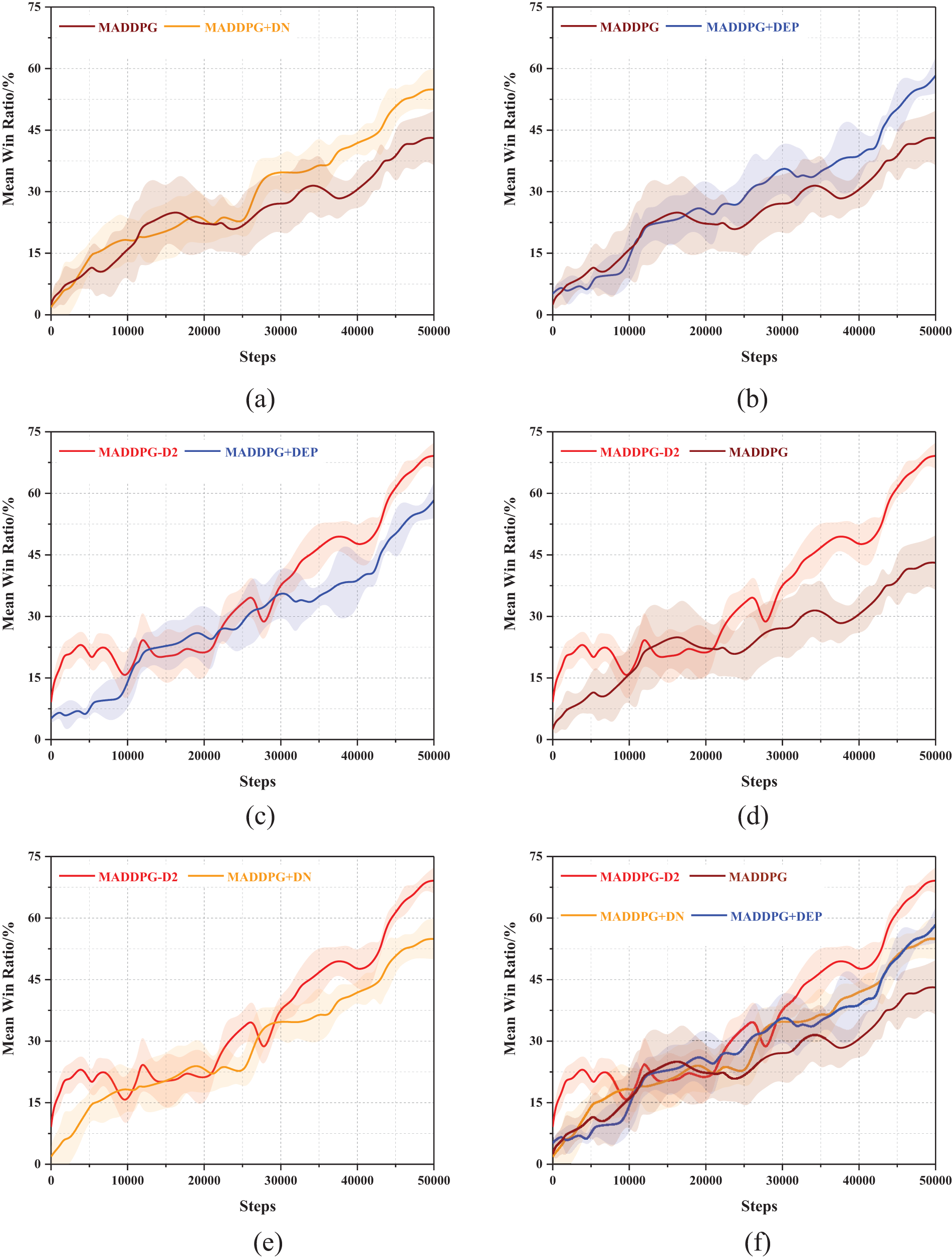
Figure 13: Comparison of the win rate curve. (a) MADDPG and MADDPG+DN; (b) MADDPG and MADDPG+DEP; (c) MADDPG-D2 and MADDPG+DEP; (d) MADDPG-D2 and MADDPG; (e) MADDPG-D2 and MADDPG+DN; (f) MADDPG-D2, MADDPG, MADDPG+DN, and MADDPG+DEP

As shown in Fig. 13, the MADDPG algorithm has the lowest win rate of 43.13%. The MADDPG-D2 algorithm with two optimization mechanisms has the highest win rate of 69.15%, which indicates that the algorithm’s performance can be effectively improved by adopting the two mechanisms because the adoption of the dual noise and dual experience pool can achieve the effective use of data and increase the exploration space, which can quickly improve to a higher win rate in a shorter number of rounds. When using a dual experience replay pool or dual noise mechanism, respectively, the performance has a certain improvement compared to the traditional MADDPG algorithm, which is mainly from a different perspective to achieve the algorithm’s win rate improvement after the training of the agents in the face of the blue side of the incoming target, they have learned to adopt a certain strategy and emerged certain tactical warfare. When the number of training rounds is 40,000, the win rate of the agents trained by the MADDPG-D2 algorithm can reach 46.31%, while the MADDPG algorithm is only 30.65%, and the overall win rate has been higher than the win rate of the MADDPG algorithm, which suggests that the MADDPG-D2 algorithm can accelerate the training of agents to a certain degree, and improve the efficiency of training.

6.4 Agent Behavior Analysis

In the process of training, the agent triggers a certain reward mechanism function, and after continuous training and strengthening, it gradually learns to effectively deal with the attack of the blue attack target, and some tactical tactics emerge.

(1)   Reasonable distribution, active and efficient interception

As shown in Fig. 14, when the blue incoming target is still at the edge of its shooting range, the untrained red agents use a lot of ammunition to fire and shoot, which may create good conditions for the subsequent secondary shooting to some extent, but due to the long distance, the missile’s interception success rate is low. At the same time, it also gives the blue targets enough maneuvering escape time, which fails to achieve a good interception effect to a certain extent. Because the red agents have not been able to judge the importance of attacking targets, they take the lead in intercepting less important targets and expose themselves prematurely. After the blue attacking targets lured the red side to fire, the subsequent organizations destroyed the exposed red units, making it difficult for the red side to deal with multi-wave attacks in the later period.

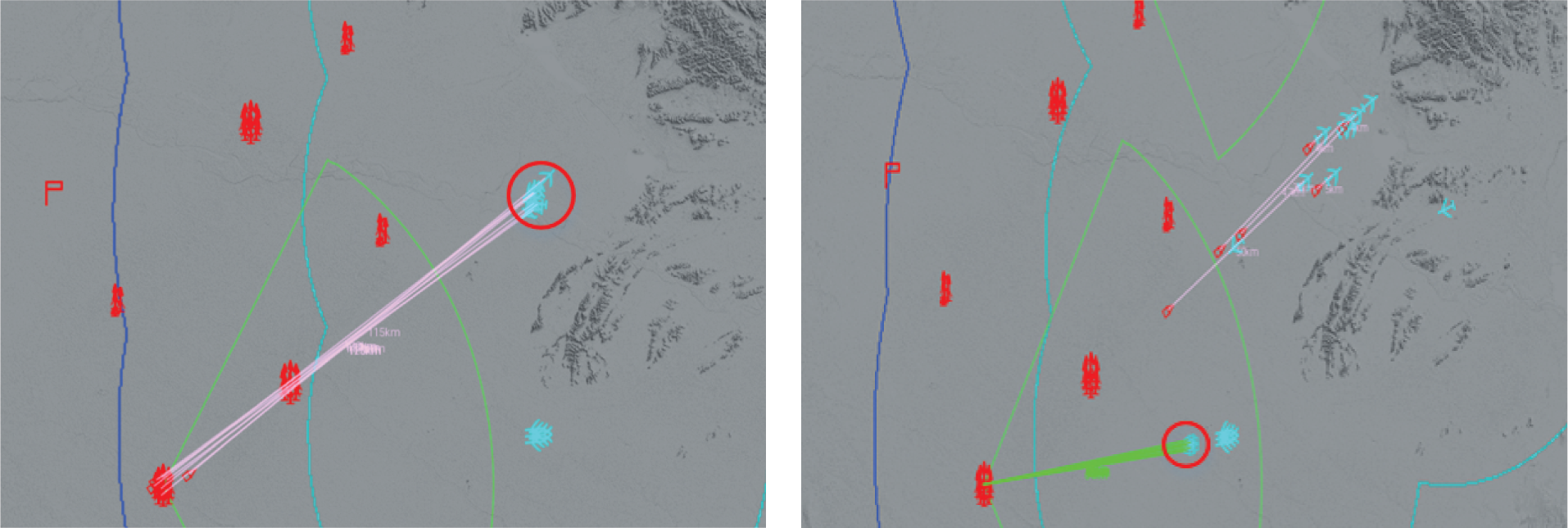
Figure 14: Before the agent training

As shown in Fig. 15, after training, the agents no longer shoot blindly but learn to intercept the incoming target reasonably and actively respond to the blue attack. The target can be intercepted one-to-many and one-to-many. Facing the attack of the first wave of blue cruise missiles, the firepower units in the defensive wing use more ammunition to intercept, while the firepower units in the strategic front of the red side use less ammunition to cooperate in intercepting the cruise missiles while avoiding side attack or pursuit to the greatest extent, improving the success rate of ammunition interception. Try to keep the interception resources in important defensive positions and near the command post, to cope with the subsequent multi-wave attacks by the blue side. At the same time, they also learn not to expose their positions prematurely and to preserve themselves to the maximum extent.

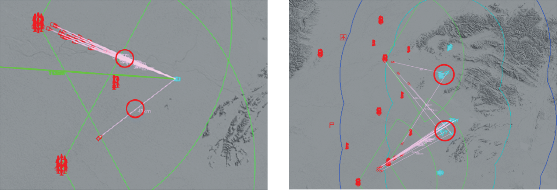
Figure 15: After the agent training

Because a fighter plane and a UAV carry multiple missiles, it takes a lot of interception resources to intercept these missiles. Therefore, the agent will intercept the blue fighter before it launches the missile to ensure its safety, which can not only achieve the set goal but also greatly save ammunition resources.

(2)   Preservation of self and active support of friendly neighbors

The long-range firepower unit agent in Fig. 16 is located at the strategic rear, and no blue attack targets have been observed around. Under the condition of ensuring the absolute safety of the defending area and sufficient ammunition, it actively responds to other firepower units and cooperates with the neighboring units in front to intercept a large number of blue attack targets, thus alleviating the defense pressure of the neighboring units. At the same time, the analysis shows that when the blue incoming missiles destroy a red fire unit, other red unit agents will provide fire assistance in time, effectively intercept the incoming missiles, and eliminate the risk of destroying neighboring units.

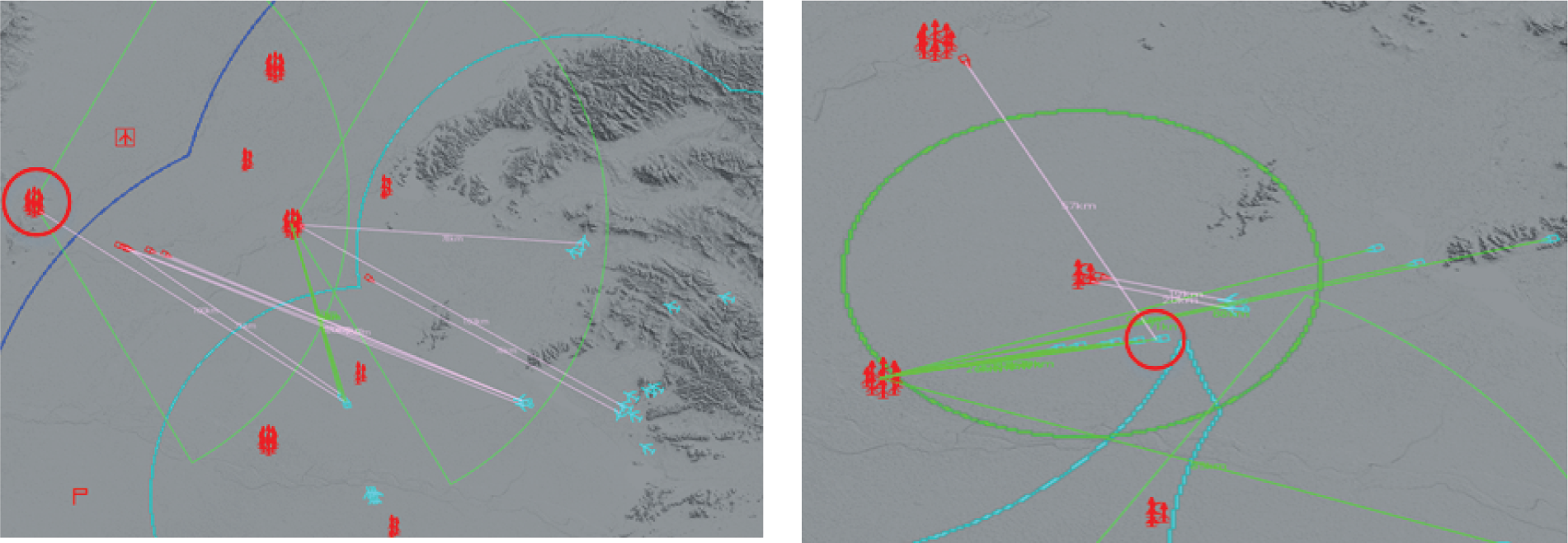
Figure 16: After the agent training

(3)   Silent ambushes, long- and short-range units working in tandem with each other

As shown in Fig. 17, after training, the agents actively participate in other defense operations while fully ensuring the absolute safety of their defense direction. In particular, the long-range and short-range firepower unit agents cooperate alternately, making full use of the advantages of long-range firepower units and accurate shooting of short-range firepower units, and cooperating to maximize the performance of firepower and ammunition. As shown in Fig. 17, in the face of a large-scale attack from the blue side, to prevent the premature exposure of their position, the long-range and short-range units keep the radars silent at the initial stage of the cruise missile attack, and when entering the ambush circle, the radars are turned on to intercept the cruise missile in real time and quickly. However, when the cruise missiles are intercepted for the first time, it is found that it is difficult to destroy them, so the short-range and long-range firepower units cooperate again and use more ammunition to intercept them until the cruise missiles are completely intercepted.

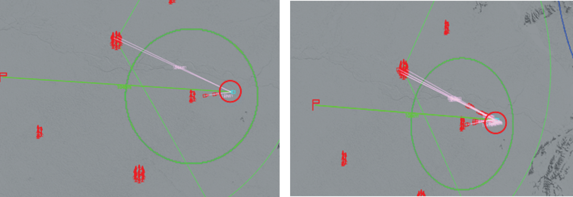
Figure 17: After the agent training

7  Conclusions

Aiming at the problem that single agent model and algorithm cannot solve the uncertainty and nonlinearity in large-scale DTA problem, this paper proposes the MADDPG-D2 algorithm based on multi-agent architecture, which increases the action exploration space and improves the data utilization rate by introducing dual noise and dual experience pool mechanism. At the same time, to speed up the initial training of agents, a pre-training method with prior knowledge is adopted. Then, based on the digital environment of ground-to-air confrontation, the real-time confrontation simulation experiment is carried out. The experimental results show that compared with the DDPG algorithm under single-agent architecture and the MADDPG algorithm under multi-agent architecture, the agents trained by the MADDPG-D2 algorithm with prior knowledge have higher win rate and average reward, and the distribution of ammunition is more reasonable. The algorithm proposed in this paper has certain advantages.

Acknowledgement: We thank our teachers, friends, and other colleagues for their discussions on simulation and comments on this paper.

Funding Statement: This research was funded by the Project of the National Natural Science Foundation of China, Grant Number 62106283.

Author Contributions: Study conception and design: Gang Wang, Qiang Fu; analysis and interpretation of results: Tengda Li; draft manuscript preparation: Tengda Li, Qiang Fu. All authors reviewed the results and approved the final version of the manuscript.

Availability of Data and Materials: The datasets used or analysed during the current study are available from the corresponding author Qiang Fu on reasonable request.

Conflicts of Interest: The authors declare that they have no conflicts of interest to report regarding the present study.

References

1. Xin B, Wang YP, Chen J. An efficient marginal-return-based constructive heuristic to solve the sensor-weapon–target assignment problem. IEEE Trans Syst Man Cybern Syst. 2019;49(12):2536–47. doi:10.1109/TSMC.2017.2784187. [Google Scholar] [CrossRef]

2. Xing HX, Xing QH. An air defense weapon target assignment method based on multi-objective artificial bee colony algorithm. Comput Mater Con. 2023;76(3):2685–705. doi:10.32604/cmc.2023.036223. [Google Scholar] [CrossRef]

3. Kline A, Ahner D, Hill R. The weapon-target assignment problem. Comput Oper Res. 2019;105:226–36. [Google Scholar]

4. Bogdanowicz ZR, Tolano A, Patel K, Coleman NP. Optimization of weapon-Target pairings based on kill probabilities. IEEE Trans Cybern. 2013;43(6):1835–44. doi:10.1109/TSMCB.2012.2231673. [Google Scholar] [PubMed] [CrossRef]

5. Zhang JD, Chen YY, Yang QM, Lu Y, Shi GQ, Wang S, et al. Dynamic task allocation of multiple UAVs based on improved A-QCDPSO. Electronics. 2022;11(7):1028. doi:10.3390/electronics11071028. [Google Scholar] [CrossRef]

6. Li GJ, He GJ, Zheng MF. Uncertain multi-objective dynamic weapon-target allocation problem based on uncertainty theory. Aims Math. 2023;8(3):5639–69. doi:10.3934/math.2023284. [Google Scholar] [CrossRef]

7. Gu J, Zhao J, Yan J, Chen X. Cooperative weapon-target assignment based on multi-objective discrete particle swarm optimization-gravitational search algorithm in air combat. J Beijing Univ Aeronaut Astronaut. 2015;41(2):252–8. doi:10.13700/j.bh.1001-5965.2014.0119. [Google Scholar] [CrossRef]

8. Peng G, Fang YW, Chen SH. A hybrid multiobjective discrete particle swarm optimization algorithm for cooperative air combat DWTA. J Optimiz. 2017;2017:1–12. doi:10.1155/2017/8063767. [Google Scholar] [CrossRef]

9. Rabbani Q, Khan A, Quddoos A. Modified Hungarian method for unbalanced assignment problem with multiple jobs. Appl Math Comput. 2019;361:493–8. doi:10.1016/j.amc.2019.05.041. [Google Scholar] [CrossRef]

10. Lu YP, Chen DZ. A new exact algorithm for the weapon-target assignment problem. Omega. 2021;98:102138. doi:10.1016/j.omega.2019.102138. [Google Scholar] [CrossRef]

11. Zhao Y, Liu JC, Jiang J, Zhen ZY. Shuffled frog leaping algorithm with non-dominated sorting for dynamic weapon-target assignment. J Syst Eng Electron. 2023;34(4):1007–19. doi:10.23919/JSEE.2023.000102. [Google Scholar] [CrossRef]

12. Chen M, Guo Y, Jin Y, Yang S, Gong D, Yu Z. An environment-driven hybrid evolutionary algorithm for dynamic multi-objective optimization problems. Complex Intell Syst. 2022;9(1):659–75. [Google Scholar]

13. Wei N, Liu MY, Cheng WB. Decision-making of underwater cooperative confrontation based on MODPSO. Sensors. 2019;19(9):2211. doi:10.3390/s19092211. [Google Scholar] [PubMed] [CrossRef]

14. Liu H, Zhang PH, Hu B, Moore P. A novel approach to task assignment in a cooperative multi-agent design system. Appl Intell. 2015;43(1):162–75. doi:10.1007/s10489-014-0640-z. [Google Scholar] [CrossRef]

15. Lecun Y, Bengio Y, Hinton G. Deep learning. Nature. 2015;521(7553):436–44. doi:10.1038/nature14539. [Google Scholar] [PubMed] [CrossRef]

16. Jiang Z, Jiaming S, Zhihao C. End-to-End deep reinforcement learning for image-based UAV autonomous control. Appl Sci. 2021;11(18):8419. doi:10.3390/app11188419. [Google Scholar] [CrossRef]

17. Zhang Z, Ong YS, Wang DQ. A collaborative multi-agent reinforcement learning method based on policy gradient potential. IEEE Trans Cybern. 2019;51(2):1015–27. doi:10.1109/TCYB.2019.2932203. [Google Scholar] [PubMed] [CrossRef]

18. Sutton RS. Learning to predict by the methods of temporal differences. Mach Learn. 1998;3(1):9–44. doi:10.1007/BF00115009. [Google Scholar] [CrossRef]

19. Han XH, Cao ZM, Liu JQ. Research into autonomous combat decision-making in assist air defense and anti-missile based on reward guiding. IEEE Trans Cybern. 2021;44(03):26–30+40. [Google Scholar]

20. Yang QM, Zhang JD, Shi GQ, Wu JW, Wu Y. Maneuver decision of UAV in short-range air combat based on deep reinforcement learning. IEEE Access. 2020;8:363–78. doi:10.1109/ACCESS.2019.2961426. [Google Scholar] [CrossRef]

21. Fu Q, Fan Ch L, Song YF, Guo XK. Alpha C2–An intelligent air defense commander independent of human decision-making. IEEE Access. 2020;8:87504–16. [Google Scholar]

22. Liu JY, Wang G, Fu Q, Yue Sh H, Wang SY. Task assignment in ground-to-air confrontation based on multi-agent deep reinforcement learning. Def Technol. 2023;19(1):210–9. doi:10.1016/j.dt.2022.04.001. [Google Scholar] [CrossRef]

23. Lu K, Li RD, Li MC, Xu GR. MADDPG-based joint optimization of task partitioning and computation resource allocation in mobile edge computing. Neural Comput Appl. 2023;35(22):16559–76. doi:10.1007/s00521-023-08527-8. [Google Scholar] [CrossRef]

24. Tian T, Ziniu L, Yang Y. Error bounds of imitating policies and environments for reinforcement learning. IEEE Trans Pattern Anal Mach Intell. 2021;44(10):6968–80. doi:10.1109/TPAMI.2021.3096966. [Google Scholar] [PubMed] [CrossRef]

25. Wen M, Topcu U. Constrained cross-entropy method for safe reinforcement learning. IEEE Trans Automat Contr. 2020;66(7):3123–37. doi:10.1109/TAC.2020.3015931. [Google Scholar] [CrossRef]