
 Submit a Paper
 Propose a Special lssue
 Open Access
ARTICLE

Composite Fractional Trapezoidal Rule with Romberg Integration
1 Department of Mathematics, Al Zaytoonah University of Jordan, Amman, 11733, Jordan
2 Nonlinear Dynamics Research Center (NDRC), Ajman University, Ajman 346, United Arab Emirates
3 Department of Mathematics, Faculty of Science, Zarqa University, Zarqa, 13110, Jordan
4 Department of Mathematics, Prince Sattam Bin Abdulaziz University, Alkharj, 11942, Saudi Arabia
5 Department of Mathematics, The University of Jordan, Amman, 11942, Jordan
* Corresponding Author: Iqbal M. Batiha. Email:
(This article belongs to the Special Issue: New Trends on Meshless Method and Numerical Analysis)
Computer Modeling in Engineering & Sciences 2024, 140(3), 2729-2745. https://doi.org/10.32604/cmes.2024.051588
Received 09 March 2024; Accepted 23 April 2024; Issue published 08 July 2024
 View Full Text
 Download PDF
Abstract
The aim of this research is to demonstrate a novel scheme for approximating the Riemann-Liouville fractional integral operator. This would be achieved by first establishing a fractional-order version of the -point Trapezoidal rule and then by proposing another fractional-order version of the -composite Trapezoidal rule. In particular, the so-called divided-difference formula is typically employed to derive the -point Trapezoidal rule, which has accordingly been used to derive a more accurate fractional-order formula called the -composite Trapezoidal rule. Additionally, in order to increase the accuracy of the proposed approximations by reducing the true errors, we incorporate the so-called Romberg integration, which is an extrapolation formula of the Trapezoidal rule for integration, into our proposed approaches. Several numerical examples are provided and compared with a modern definition of the Riemann-Liouville fractional integral operator to illustrate the efficacy of our scheme.Keywords
Mathematical modeling of technical problems and chemical, physical, and economic phenomena [1,2] can all benefit from the utilization of fractional calculus [3]. As a result, a variety of definitions of fractional-order operators have been established recently. Such operators have played crucial roles in advancing various subjects and practical applications in the field of applied mathematics (see [4,5]). Researchers have studied numerous modern developments in fractional calculus theory, exploring their potential applications in a variety of scientific and engineering fields. The fundamentals of fractional calculus have been particularly recognized as significant mathematical tools for describing numerous actual applications [6]. As a consequence, numerous researchers have developed and approved a variety of fractional-order differentiators and integrators, see [7–10].
It is essential to emphasize that fractional-order differentiators have two primary operators, the Riemann-Liouville derivative operator and the Caputo derivative operator, which are both methods that relate to the local derivative of a function [11]. The Caputo differentiator has been shown to be superior to the Riemann-Liouville differentiator for a number of real-world applications [12,13], despite the divergent views of many mathematicians [14,15]. This is because it can be used with certain supposed initial conditions once taking the derivatives of fractional-order [16,17].
The Riemann-Liouville integrator is regarded as an inverse operator for both former operators, regardless of which one is better. This is because the Caputo differentiator is an enhanced formula from the Riemann-Liouville differentiator [11,12]. The fractional-order integrator assumes that various elements cannot be coordinated and are continuously identical. Typically, we use the fractional-order integrator to represent an indefinite integral. Previous attempts to come up with a more general version of the fundamental theorem in fractional calculus were limited, with only two successful attempts [18,19]. However, [18] did come up with a number of different versions of this theorem. The researchers in [19] presented a further coordinated approach, but they did not address the fractional definite integral definition. Similarly, the formulations in [20,21] also lacked a clear definition of the fractional definite integral.
Apart from the research done by Ortigueira et al. and Machado et al. [22], which introduced a definition of the fractional definite integral and analyzed the major theorem of fractional calculus, no other formulations have been made [23]. Given this background and following the approach in classical numerical analysis, this paper aims to establish a novel formulation, referred to as the composite fractional formula, for providing a good approximation for the definite fractional integral, specifically the Riemann-Liouville fractional integrator. Such an operator will be approximated using a 3-point central fractional formula, which will be derived by employing the definite fractional integral definition proposed by O. Manuel and J. Machado’s in conjunction with the generalized Taylor’s formula. Subsequently, the aforementioned formula will be further extended to
We arrange the subsequent portions of this article as follows: Section 2 offers a concise overview of the fundamental concepts and definitions of fractional calculus. Section 3 talks about the main results of this study and how the
In this portion, certain fundamental definitions and vital preliminaries regarding fractional calculus are reviewed. This really prepares to our principal results later on.
Definition 1. [24,25] The Riemann-Liouville fractional integrator of a function
where
In the forthcoming content, we recollect specific features of Riemann-Liouville fractional integrator for the sake of completeness:
Definition 2. [24,25] The Caputo fractional differentiator of a function h(u) be declared as
where
Some of Caputo differentiator properties are outlined in the following content for the sake of completeness [24,25]:
Furthermore, we present below additional properties associated with the composition of the prior two operators [24,25]:
and
where
Definition 3. [24,25] By means of Riemann-Liouville fractional integrator, the Caputo fractional differentiator of a function
where
In the following content, we remember two highly significant results that would play a crucial role in establishing the primary outcomes of this study. The first one is attributed to M. Ortigueira and J. Machado, who developed an accurate formula for determining exact values of definite fractional integrals [23]. On the other hand, the second result pertains to Odibat and Momani, who provided a generalisation of the renowned Taylor theorem [25].
Definition 4. [23] The definite fractional integral of the function
where
Theorem 1. [26] (Divided-difference formula) Assume that
where
for
In this section, we intend first to establish a fraction-order version of the
Theorem 2. (The
where
Proof. To show this result, we apply directly on the divided-difference formula reported in Theorem 1 to get
or
Accordingly, by utilizing the definite fractional integral reported in Eq. (13), we obtain
Considering the sense of divided-difference coupled with assuming
or
This consequently implies
or
Hence, by replacing back
Corollary 1. Under the same assumptions of Theorem 2 with
where
Proof. Note that supposing
i.e.,
After some calculations, we obtain
or
which consequently implies the desired result. ■
Theorem 2. (The
where
Proof. To prove this result, we use again the definite fractional integral reported in Eq. (13) to obtain
Now, with the use of the 2-point fractional Trapezoidal Rule reported in Eq. (16), we get
This immediately implies
or
which is equivalent to the desired result. ■
Corollary 2. Under the same assumptions of Theorem 2 with
Proof. Omitted. ■
The
The Romberg integration method utilizes the composite Trapezoidal rule to obtain initial approximations and subsequently implements the Richardson extrapolation procedure to enhance these approximations. It is worth noting that Richardson extrapolation might be applied to any approach that has the form
where
In a similar manner, we can state the
where
Solving Eqs. (38) and (43) yields
Now, supposing
which is called Romberg integration for approximating
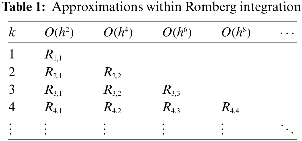
All approximations within Romberg integration reported in Table 1 are listed below for completeness:
where the denominator can be found via
The challenges that we encountered in adapting Romberg integration to the fractional calculus context may be summarized as follows:
1. For some combined functions resulting from the computational operations, Romberg integration causes more computational complexity. Actually, to avoid this, we handled some functions that lacked this issue, and we are looking to improve our current work to be adapted to all functions, even if they are complex.
2. The discontinuities of functions within the interval pose challenges for Romberg integration, and to handle such a situation, we have adapted the step size chosen in our approach.
Based on the previous discussion, we believe that the approximation of fractional integrals can be improved by the development of the composite fractional Trapezoidal rule with Romberg integration. In particular, the composite fractional Trapezoidal rule with Romberg integration provides a robust numerical method for computing the fractional integrals, allowing researchers to analyze and model complex systems exhibiting fractional dynamics, which have applications in various scientific and engineering fields. Also, the composite fractional Trapezoidal rule with Romberg integration can be integrated with other numerical techniques for solving fractional differential equations, integral equations, or even optimization problems.
This section aims to confirm the adequacy of our last proposed formula, the composite fractional Trapezoidal rule with Romberg integration, for approximating the Riemann–Liouville fractional integral operator for several functions. Tables are used to show and compare about the acquired discoveries.
In the following content, we discuss two numerical examples which would confirm the validity of the proposed scheme in comparison with the results gained by Ortigueira et al. [23].
Example 1. Let us consider the main function is
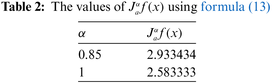
In what follows, we depict respectively two tables (Tables 3 and 4) that include approximate values for
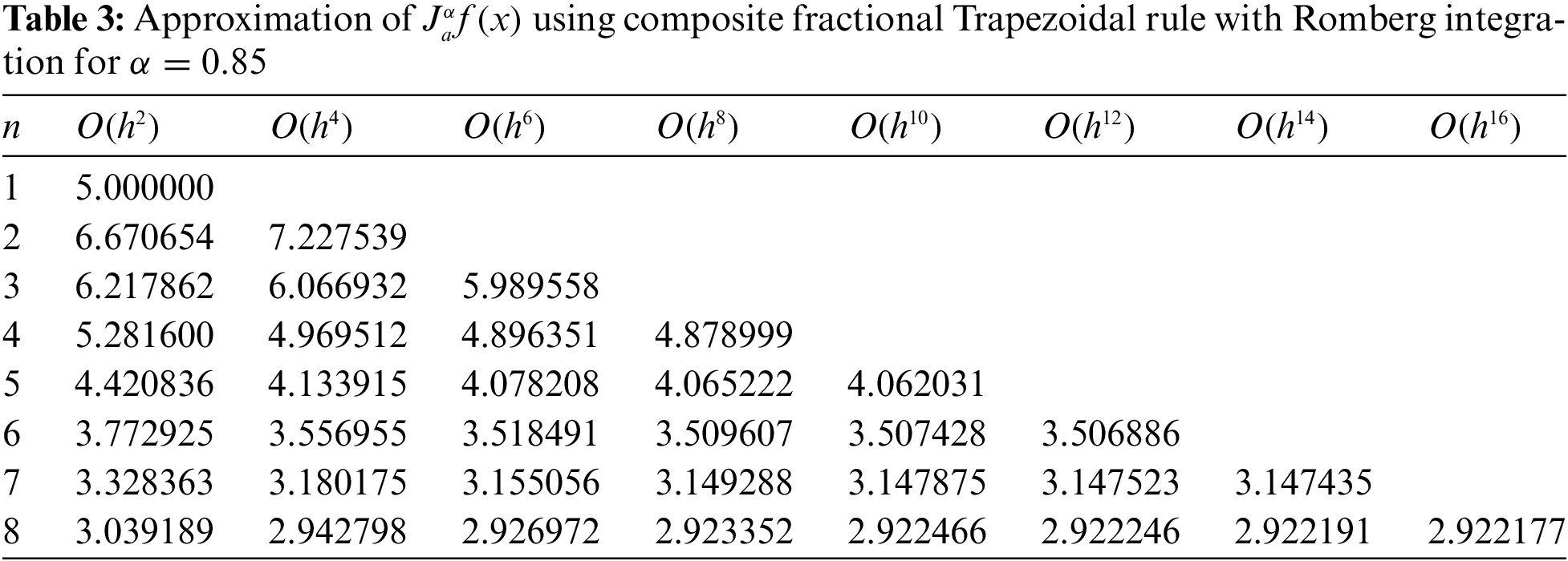
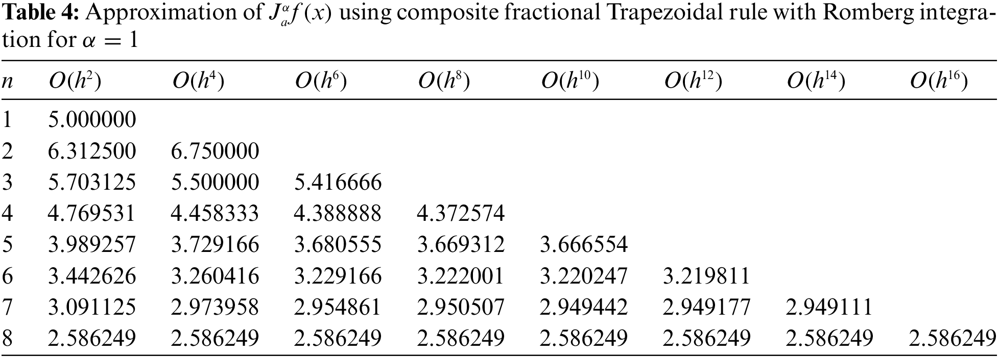
It should be noticed here that the last two approximated values generated in Tables 3 and 4 using the proposed composite fractional Trapezoidal rule with Romberg integration are very close to the values of
Example 2. Let us consider here the function is
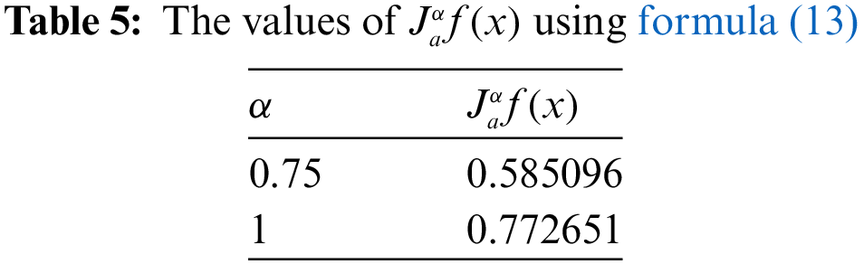
In Tables 6 and 7 listed below, we provide respectively the gained approximate results for
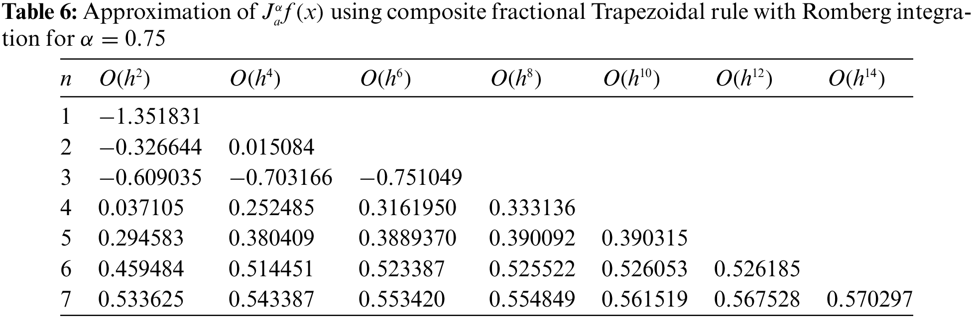
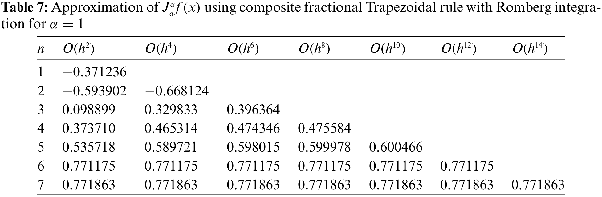
In light of the two approximated values provided at the end of Tables 6 and 7 obtained by using the proposed composite fractional Trapezoidal rule with Romberg integration, we can assert that those values are very close to the values of
In the subsequent content, we provide further numerical examples with the aim of illustrating the success of our proposed method against the failure of formula (13) in approximating
On the other hand, our proposed composite fractional Trapezoidal formula with Romberg integration have worked appropriately in approximating
Example 3. Consider here the main function is
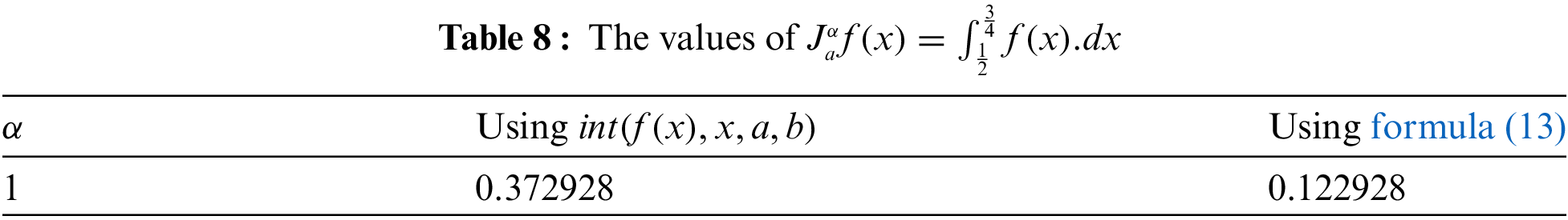
Based on Table 8, one might easily observe the big error that can be gained from using formula (13) in comparison with the value offered by “
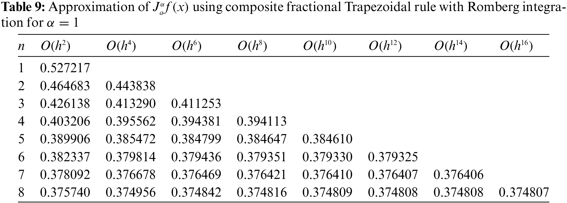
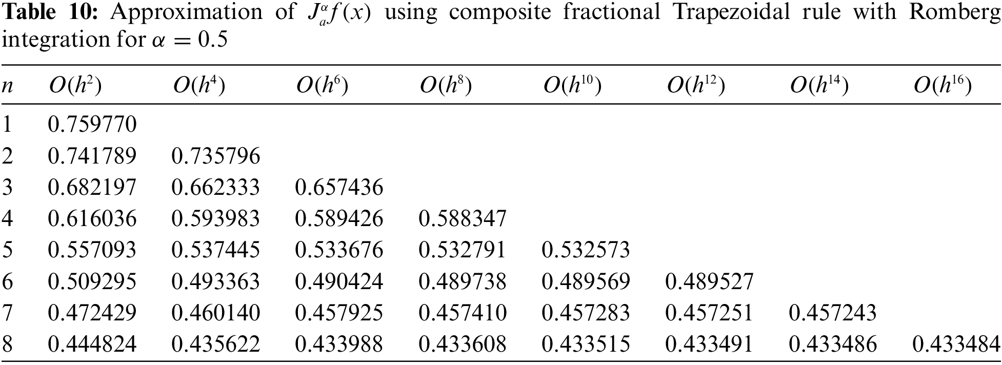
In view of the previous numerical results, one can obviously notice that the last approximate value in Table 9 is very close to the value of
Example 4. Consider
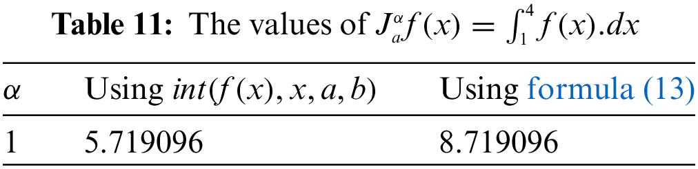
On the basis of 11, we notice that there is a big error from using formula (13) in comparison with the value offered by “
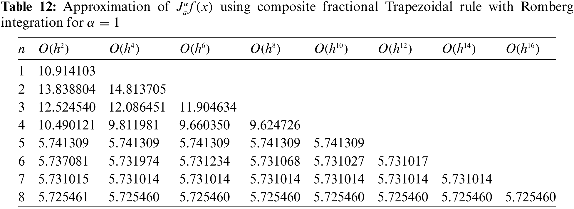
In light of the previous discussion, it can be clearly observed that the approximate value located at the end of Table 12 is very close to the value of
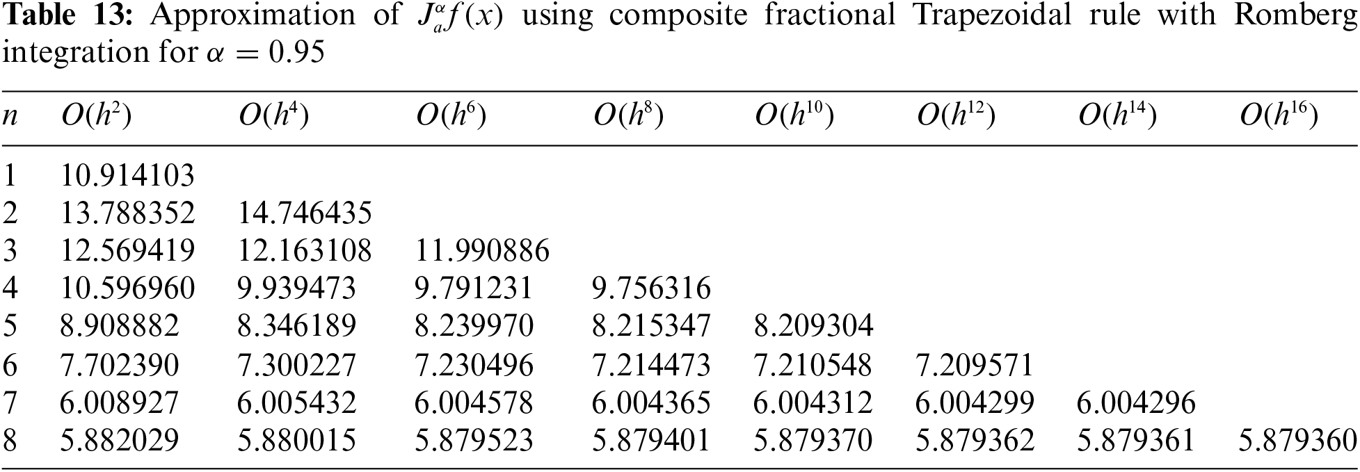
Example 5. Consider
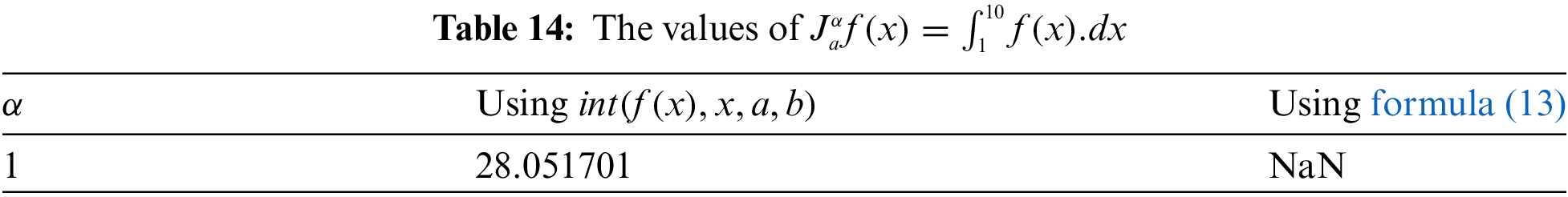
In consideration of 14, we notice that there is no value from using formula (13) in comparison with the value 28.051701 offered by “
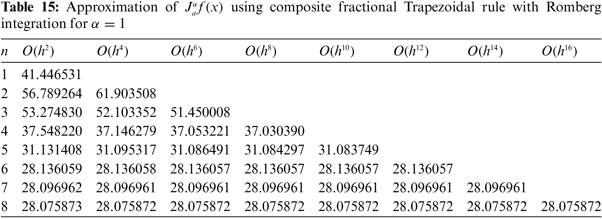
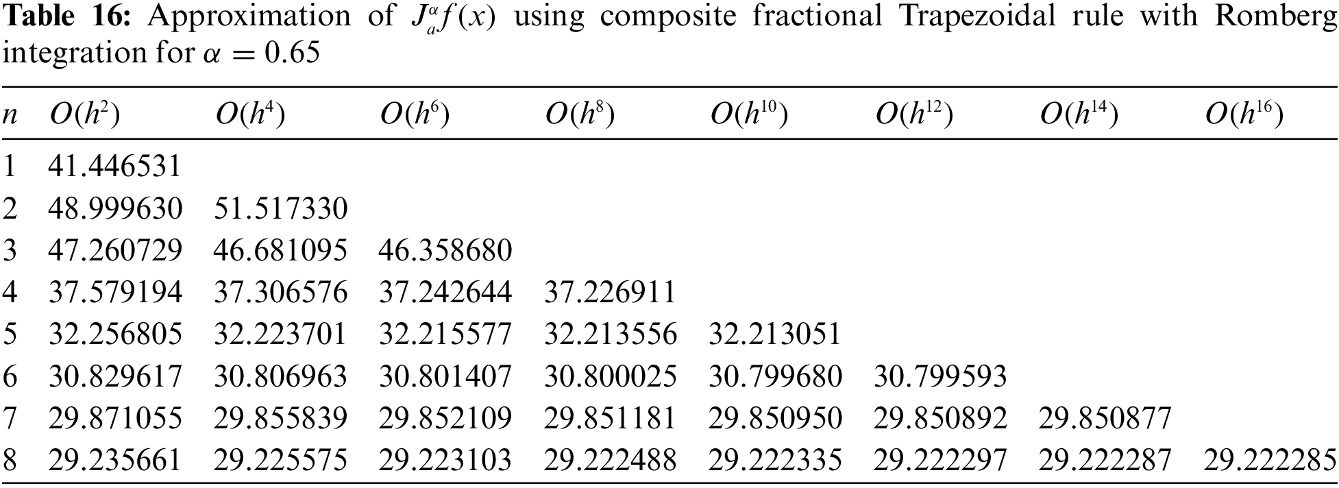
From the previous discussion, it can be clearly observed that the approximate value located at the end of Table 15 is very close to the value of
A final remark that should be stated here is that the changes in the fractional order have significant effects on the performance of the composite fractional Trapezoidal rule with Romberg integration. As one can see from the given numerical examples, the closer the value of the fractional order is to 1 for a given function, the closer we are to the classical integral of that function. Also, we believe that the composite fractional Trapezoidal rule with Romberg integration may be used as an alternative numerical method for solving integral equations, fractional differential equations, or even optimization problems that arise in physics, control theory, modeling biological systems, fractional optimal control problems, modeling electrochemical processes, fractional partial differential equations, and many others.
This paper has successfully established a novel approach for finding a good approximation for the Riemann-Liouville fractional integrator. Specifically, we have successfully derived the so-called
Acknowledgement: None.
Funding Statement: The authors received no specific funding for this study.
Author Contributions: The authors confirm contribution to the paper as follows: study conception and design: I.M. Batiha, R. Saadeh; data collection: I.H. Jebril; analysis and interpretation of results: I.M. Batiha, A. Qazza; draft manuscript preparation: A.A. Al-Nana, S. Momani. All authors reviewed the results and approved the final version of the manuscript.
Availability of Data and Materials: No new data were created or analysed in this study. Data sharing is not applicable to this article.
Conflicts of Interest: The authors declare that they have no conflicts of interest to report regarding the present study.
References
1. Aho AV, Hopcroft JE, Ullman JD. The design and analysis of computer algorithms. Boston: Addison-Wesley; 1974. [Google Scholar]
2. Rajagopal K, Hasanzadeh N, Parastesh F, Hamarash II, Jafari S, Hussain I. A fractional-order model for the novel coronavirus (COVID-19) outbreak. Nonlinear Dyn. 2020;101(1):711–8. doi:10.1007/s11071-020-05757-6. [Google Scholar] [PubMed] [CrossRef]
3. Williams WK, Vijayakumar V, Nisar KS, Shukla A. Atangana-Baleanu semilinear fractional differential inclusions with infinite delay: existence and approximate controllability. ASME J Comput Nonlinear Dynam. 2023;18(2):021005. doi:10.1115/1.4056357. [Google Scholar] [CrossRef]
4. Saadeh R, Ala’yed O, Qazza A. Analytical solution of coupled hirota-satsuma and KdV equations. Fractal Fract. 2022;6(12):694. doi:10.3390/fractalfract6120694. [Google Scholar] [CrossRef]
5. Saadeh R, Abu-Ghuwaleh M, Qazza A, Kuffi E. A fundamental criteria to establish general formulas of integrals. J Appl Math. 2022;2022(1):6049367. doi:10.1155/2022/6049367. [Google Scholar] [CrossRef]
6. Hamadneh T, Hioual A, Alsayyed O, Al-Khassawneh YA, Al-Husban A, Ouannas A. Finite time stability results for neural networks described by variable-order fractional difference equations. Fractal Fract. 2023;7(8):616. doi:10.3390/fractalfract7080616. [Google Scholar] [CrossRef]
7. Batiha IM, Alshorm S, Al-Husban A, Saadeh R, Gharib G, Momani S. The n-point composite fractional formula for approximating Riemann-Liouville integrator. Symmetry. 2023;15(4):938. doi:10.3390/sym15040938. [Google Scholar] [CrossRef]
8. Batiha IM, Alshorm S, Jebril I, Zraiqat A, Momani Z, Momani S. Modified 5-point fractional formula with Richardson extrapolation. AIMS Math. 2023;8(4):9520–34. doi:10.3934/math.2023480. [Google Scholar] [CrossRef]
9. Albadarneh RB, Batiha IM, Adwai A, Tahat N, Alomari AK. Numerical approach of Riemann-Liouville fractional derivative operator. Int J Electr Comput Eng. 2021;11(6):5367–78. doi:10.11591/ijece.v11i6.pp5367-5378. [Google Scholar] [CrossRef]
10. Albadarneh RB, Batiha I, Alomari AK, Tahat N. Numerical approach for approximating the Caputo fractional-order derivative operator. AIMS Math. 2021;6(11):12743–56. doi:10.3934/math.2021735. [Google Scholar] [CrossRef]
11. Hilfer R, Luchko Y, Tomovski Z. Operational method for the solution of fractional differential equations with generalized Riemann-Liouville fractional derivatives. Fract Calc Appl Anal. 2009;12(3):299–318. [Google Scholar]
12. Baleanu D, Wu GC, Zeng SD. Chaos analysis and asymptotic stability of generalized Caputo fractional differential equations. Chaos, Solit Fractals. 2017;102:99–105. doi:10.1016/j.chaos.2017.02.007. [Google Scholar] [CrossRef]
13. Sene N, Ndiaye A. On class of fractional-order chaotic or hyperchaotic systems in the context of the Caputo fractional-order derivative. J Math. 2020;2020(22):8815377–15. doi:10.1155/2020/8815377. [Google Scholar] [CrossRef]
14. Sene N. Fractional advection-dispersion equation described by the Caputo left generalized fractional derivative. Palestine J Math. 2021;10(2):562–79. [Google Scholar]
15. Altan G, Alkan S, Baleanu D. A novel fractional operator application for neural networks using proportional Caputo derivative. Neural Comput Appl. 2023;35(4):3101–14. doi:10.1007/s00521-022-07728-x. [Google Scholar] [CrossRef]
16. Qazza A, Saadeh R, Salah E. Solving fractional partial differential equations via a new scheme. AIMS Math. 2022;8(3):5318–37. doi:10.3934/math.2023267. [Google Scholar] [CrossRef]
17. Saadeh R, Abdoon M, Qazza A, Berir M. A numerical solution of generalized Caputo fractional initial value problems. Fractal Fract. 2023;7(4):332. [Google Scholar]
18. Grigoletto EC, de Oliveira EC. Fractional versions of the fundamental theorem of calculus. Appl Math. 2013;4(7):34039. [Google Scholar]
19. Tarasov VE. Fractional vector calculus and fractional Maxwell’s equations. Ann Phys. 2008;323:2756–78. [Google Scholar]
20. Kilbas AA, Srivastava HM, Trujillo JJ. Theory and applications of fractional differential equations. Amsterdam: Elsevier; 2006. [Google Scholar]
21. Samko SG, Kilbas AA, Marichev OI. Fractional integrals and derivatives: theory and applications. London: Gordon and Breach Science Publishers; 1993. [Google Scholar]
22. Machado JT, Mainardi F, Kiryakova V. Fractional calculus: Quo Vadimus? (where are we going?). Fract Calc Appl Anal. 2015;18(2):495–526. [Google Scholar]
23. Ortigueira M, Machado J. Fractional definite integral. Fractal Fract. 2017;1(1):2. [Google Scholar]
24. Batiha IM, El-Khazali R, AlSaedi A, Momani S. The general solution of singular fractional-order linear time-invariant continuous systems with regular pencils. Entropy. 2018;20(6):400. [Google Scholar] [PubMed]
25. Odibat ZM, Momani S. An algorithm for the numerical solution of differential equations of fractional order. J Appl Math Inform. 2008;26(1–2):15–27. [Google Scholar]
26. Burden RL, Faires JD. Numerical analysis. 9th ed. Boston: Thomson Brooks/Cole; 2005. [Google Scholar]
27. Allahviranloo T. Romberg integration for fuzzy functions. Appl Math Comput. 2005;168(2):866–76. [Google Scholar]
28. Saadeh R, Qazza A, Burqan A. A new integral transform: ara transform and its properties and applications. Symmetry. 2020;12(6):925. [Google Scholar]
29. Liu A, Yasin F, Afzal Z, Nazeer W. Analytical solution of a non-linear fractional order SIS epidemic model utilizing a new technique. Alex Eng J. 2023;73:123–9. [Google Scholar]
30. Umapathy K, Palanivelu B, Leiva V, Dhandapani PB, Castro C. On fuzzy and crisp solutions of a novel fractional pandemic model. Fractal Fract. 2023;7(7):528. doi:10.3390/fractalfract7070528. [Google Scholar] [CrossRef]
31. Chakir Y. Global approximate solution of SIR epidemic model with constant vaccination strategy. Chaos Solit Fract. 2023;169(772):113323. doi:10.1016/j.chaos.2023.113323. [Google Scholar] [CrossRef]
Cite This Article
 Copyright © 2024 The Author(s). Published by Tech Science Press.
This work is licensed under a Creative Commons Attribution 4.0 International License , which permits unrestricted use, distribution, and reproduction in any medium, provided the original work is properly cited.
 Downloads
 Citation Tools