Enhancing Critical Path Problem in Neutrosophic Environment Using Python

1  Introduction

Planning multiple tasks to develop and execute the project within the allotted time frame is an essential part of project management [1]. Time restrictions are a common source of failure while working manually in many industries. Project managers use scheduling tools like Gantt charts and network planning to address such issues. Previous researchers were involved in the study of Gantt charts due to their less complex nature. Furthermore, large-scale and more complicated project execution has emerged since 1950, leading to the development of project management models, i.e., network analysis.

Network analysis deals with the coordination of project scheduling and the identification of task interdependencies to design and analyze [2]. This analytical framework employs two primary methodologies: the CPM (Critical Path Method) and the PERT (Program Evaluation and Review Technique). Kelly and Walker created CPM [3], which provides definitive project execution schedules in a chronological pattern based on deterministic time estimation [4]. PERT was created by Malcolm et al. [5] and is also called the backward research method [6] because it has a three-time estimation that takes the account of uncertainty [7]. Our study examines the critical path problem (CPP) using the CPM approach, which is a common method in project management, to distinguish between critical and non-critical tasks. This makes it easier to solve problems and avoid delays. CPP improves the project’s efficiency by helping to determine the minimum feasible time for task completion [8]. Utilizing CPP involves a multitude of operational metrics, including the calculation of the maximum time allowance, the earliest and latest initiation, and the corresponding completion time [9]. Traditional CPP practices dictate that fixed-time estimations represent this project activity. However, predicting future events in the real world is difficult due to the inherent unpredictability of dynamic project environments [10].

An anthology of researchers demonstrated the classical critical path problem (CCPP) study in project scheduling across a variety of domains. However, improving project management and control in the CCPP faces challenges in anticipating and estimating parameters involving uncertainty to calculate time deviations. In such a scenario, Zadeh introduced the concept of fuzzy logic to address the limitations of classical set theory while dealing with the study of vagueness and uncertainty in real-world situations [11]. Following up on Zadeh’s theory, Atanassov [12] introduced the legerdemain concept of intuitionistic fuzzy sets (IFS) in 1986, involving both membership and non-membership functions. To advance the study of uncertainty, researchers developed triangular fuzzy numbers (TrFN) [13] and trapezoidal fuzzy numbers (TFN) [14] to represent uncertainty. More fuzzy numbers have been made, like octagonal [15], heptagonal [16], and hendecagonal [17]. This shows that the research has gone beyond the initial forms. Researchers further conducted the study to extend zadeh’s pioneering work in fuzzy logic to a variety of practical applications. In one of these efforts, Mehlawat et al. [18] used IFS to study multi-criteria decision-making (MCDM) for critical path selection. An advanced methodology to implement fuzzy methods to handle the challenges of project management. Another study by Revathi et al. [17] showed how flexible and useful fuzzy critical path problems (FCPP) in managing agricultural projects. It uses a variety of fuzzy parameters, such as trapezoidal, heptagonal, and hendecagonal fuzzy numbers, to accurately handle the complexity of agricultural data. Senussi et al. [19] also used the TFN parametric form to account for uncertainty in planning projects that will make important contributions to the field. Ganesan et al. [20] analyzed another notable study of inter-valued parameters in operational networks. Further, many studies have implemented fuzzy environments in different optimization techniques such as supply chain [21], transportation [22] and so on. Although fuzzy logic has improved, it cannot fully capture real-world uncertainty. There are still unresolved issues while solving CCPP and FCPP under uncertain circumstances. This shift is being driven to address the research gaps leading to neutrosophic logic.

To adopt such parameters, Smarandache [23] introduced the neutrosophic set (NS) in 1998 with three integrands: truthiness, indeterminacy, and falsity, unlike the general fuzzy and IFS. With the daily progress of research, Wang et al. [24] proposed a single-valued neutrosophic set (SVNS) that solves complex problems by involving the study of uncertain parameters. Investigations by Chakraborty et al. [25,26] examined different categories of trapezoidal and triangular neutrosophic numbers. Fernandez et al. [27] and Abdel-Basset et al. [28] looked into the method using a single-valued trapezoidal neutrosophic number (SVTNN); this technique employs neutrosophic PERT (NPERT) to effectively navigate unpredictable settings via network analysis. Based on these findings, Nagalakshmi et al. [29] compared the study of NS and FCPP. This comparative research shows that neutrosophic sets can provide greater versatility in risk assessment. Another work by Priyadharsini et al. [30] evaluated triangular NPERT analysis for estimating project time and costs. A lot of researchers are studying NS under different optimization methods, such as the shortest path [31], minimum spanning tree [32], MCDM [33], linear programming problem [34], and so on. In addition to their theoretical and practical uses, ongoing research also uses computer implementations of these advanced ideas. These have greatly improved tools, such as the NCMPy package for managing neutrosophic cognitive maps [35] and the open-source python neutrosophic package [36], which are based on this theoretical base. The main study is about how to solve CPP in a neutrosophic environment using the python programming language. This will enhance the effectiveness and efficiency of computing environments by enabling the effective application of neutrosophic understanding.

The following is a list of the key research contributions to the development of the CPP objective:

•   According to recent literature, CPP solves complex problems by including uncertainty study.

•   To represent uncertainty, our proposed model uses CPP in a neutrosophic environment (NCPP). It uses a single-valued triangular neutrosophic number (TrSVNN) to represent the uncertainty and ambiguity that come with project timelines. Furthermore, the initiation also addresses a new set of problems with varying uncertainty parameters.

•   The task involves implementing a score function that aims to quantify the accuracy of project analysis.

•   Developed the proposed methodology in python, a computational programming language, to elucidate the nuances of neutrosophic logic.

•   Implementing a comparative analysis that reveals neutrosophic logic’s superior capabilities over classical and fuzzy in demonstrating its enhanced effectiveness while dealing with uncertainty and complexity.

1.1 Study Novelty

In recent years, there has been an increasing focus within the academic community on developing the study of the neutrosophic field to discover innovative applications in varied domains. Despite the progress in understanding and applying TrSVNN, a multitude of unresolved theories and challenges continue to persist. The primary objective of this research article is to shed light on the concepts of the neutrosophic domain and offer a novel viewpoint on its possible applications. Our novelty includes:

•   Developed a novel approach while employing TrSVNN, an effective and simple model for handling uncertain information.

•   The literature utilizes a scoring approach under neutrosophic study as a further extension of FCPP.

•   A comparative study analysis is conducted on our proposed model to that of previous existing FCPP and CCPP models.

•   An innovation to this study is the use of python for computational execution, which aids in better quality decision-making.

1.2 Structure of the Paper

The structure of the article unfolds as follows: Section 2 defines the prelims useful for the development of the document. Section 3 gives the methodology about the existing classical and neutrosophic environment, where the discussion of classical critical path is derived in Subsection 3.1 and introduces the proposed devlopment of neutrosophic formulation on the working principle of CPP mentioned in Subsection 3.2 and the proposed algorithmn is breifly discussed in Subsection 3.3. Further, Section 4 solves numerical example study that provides existing CCPP in Section 4.1 and solves existing literature in Section 4.2, further the new set of problem of NCPP using three different cases was implemented in Subsection 4.3 and lastly conclusion.

2  Preliminary

The paper includes a background on the fundamental concepts of FS, NS, TrSVNN is as follows:

Definition 2.1. Fuzzy Set [11]: A set v~, generally obtained as v~={(θ,μv~(θ)):θ∈ν,μv~(θ)∈[0,1]}, represented by the ordered pair (θ,μv~(θ)), where θ be the member of set v~ and 0≤μv~(θ)≤1.

Definition 2.2. Neutrosophic Set (NS) [23]: A set v~ns is the universal domain of a set ν, symbolically stated as θ is known to be a neutrosophic set (NS), if v~ns={⟨θ;[δv~ns(θ),φv~ns(θ),γv~ns(θ)]⟩⋮θ∈ν}, where δv~ns(θ),φv~ns(θ),γv~ns(θ):ν→]−0,1+[ symbolizes the truth δv~ns(θ), indeterminacy φv~ns(θ), and falsity γv~ns(θ) in the decision making, that satisfies the condition: −0≤δv~ns(θ)+φv~ns(θ)+γv~ns(θ)≤3+.

Definition 2.3. Triangular Single-Valued Neutrosophic Number (TrSVNN) [25]: TrSVNN is defined as wN=⟨(h1,q1,t1);deN,eeN,feN⟩ having truth, indeterminacy, and falsity membership functions, defines as deN,eeN,feN∈[0,1].

TeN(θ)={deN(θ−h1)q1−h1h1≤θ<q1deNθ=q1deN(t1−θ)t1−q1q1<θ≤t10OtherwiseIeN(θ)={q1−θ+eeN(θ−h1)q1−h1h1≤θ<q1eeNθ=q1θ−q1+eeN(t1−θ)t1−q1q1<θ≤t11Otherwise

FeN(θ)={q1−θ+feN(θ−h1)q1−h1h1≤θ<q1feNθ=q1θ−q1+feN(t1−θ)t1−q1q1<θ≤t11Otherwise

In special case, when eeN=0, feN=0 then it reduces the fuzzy number ⟨(h1,q1,t1);deN⟩.

Definition 2.4. Comparison between two SVTNN [37]: Consider two SVTNN as e1N and j1N; where e1N and j1N are defined respectively as follows: e1N=⟨(h1,q1,t1,s1);de1N,ee1N,fe1N⟩ and j1N=⟨(h2,q2,t2,s2);dj1N,ej1N,fj1N⟩.

1.    E ′(e1N)<E ′(j1N), where e1N is smaller than j1N and symbolized as e1N<j1N;

2.    If E ′(e1N)=E ′(j1N), such that

A ′(e1N)<A ′(j1N), where e1N is smaller than j1N and symbolized as e1N<j1N;

A ′(e1N)=A ′(j1N), i C ′(e1N)<C ′(j1N), where e1N is smaller than j1N and symbolized as e1N<j1N;

E ′(e1N)>E ′(j1N), where e1N is greater than j1N and symbolized as e1N>j1N.

where ePN=⟨(hp,qp,tp,sp);dpN,epN,fpN⟩, where (p=1,2).

1.    Score function is defined as: E ′(ePN)=(hp+2qp+2tp+sp)6∗(2+dpN−epN−fpN)3

2.    Accuracy function is defined as: A ′(ePN)=(hp+2qp+2tp+sp)6∗(dpN−epN)

3.    Certainty function is defined as: C ′(ePN)=(hp+2qp+2tp+sp)6∗(dpN)

Note: If the SVTNN ePN=⟨(hp,qp,tp,sp);dpN,epN,fpN⟩ is symmetric, then qp=tp is convertible to TrSVNN.

Definition 2.5. Arithmetic operations between two (TrSVNN) [38]: Let eN and jN be the two TrSVNN represented as eN=⟨(h1,q1,t1);deN,eeN,feN⟩, jN=⟨(h2,q2,t2);djN,ejN,fjN⟩.

•   Addition: eN⊕jN=⟨(h1+h2,q1+q2,t1+t2);min(deN,djN),max(eeN,ejN),max(feN,fjN)⟩

•   Subtraction: eN⊖jN=⟨(h1−h2,q1−q2,t1−t2);min(deN,djN),max(eeN,ejN),max(feN,fjN)⟩

Definition 2.6. Binary operations between two (TrSVNN): Let eN and jN be the two TrSVNN represented as eN=⟨(h1,q1,t1);deN,eeN,feN⟩, jN=⟨(h2,q2,t2);djN,ejN,fjN⟩ be two TrSVNN, then using the score function defined from Definition 2.4 is as follows:

eN+jN=⟨(h1+h2,q1+q2,t1+t2);min(deN,djN),max(eeN,ejN),max(feN,fjN)⟩

E ′(eN+jN) =((h1+h2)+4(q1+q2)+(t1+t2)6) ∗(2+min(deN,djN)−max(eeN,ejN)−max(feN,fjN)3)

2.1 List of Abbreviation Used throughout This Paper

•   CPP represents “critical path problem”.

•   TrFN represents “triangular fuzzy number”.

•   TFN represents “trapezoidal fuzzy numbers”.

•   TrIFS represents “triangular intuitionistic fuzzy sets”.

•   CCPP represents “classical critical path problem”.

•   NS represents “neutrosophic set”.

•   TrSVNN represents “single-valued triangular neutrosophic number”.

•   SVTNN represents “single-valued trapezoidal neutrosophic number”.

•   CP represents “critical path”.

•   NPP represents “neutrosophic non-critical possible paths”.

•   NCPP represents “neutrosophic critical path problem”.

•   NCPL represents “neutrosophic critical path length”.

•   NCP represents “neutrosophic critical path”.

•   CCPL represents “critical crisp path length”.

•   FCPP represents “fuzzy critical path problems”.

•   FCP represents “fuzzy critical path”.

•   FCPL represents “fuzzy critical path length”.

3  Methodology

The exploration to delve the study of existing CCPP and the proposed NCPP is discussed above to enhance the decision-making framework in addressing the uncertainty in project scheduling.

3.1 Existing Critical Path Network Problem Formulation under Classical Environment

The CCPP implements a dynamic programming in the network, a cyclic-directed graph G=(V,A). In this graph, V is the set of vertices with numbers from 1 (source) to m (destination), and A is the set of directed edges. The project initialization starts with zero, indicating that there is no accumulated duration at the beginning.

f(m)=0f(k)=maxk<δ{Ckδ+f(δ)|<k,δ>∈A}(3.1)

The weight Ckδ of the directed edge from one vertex k to another vertex δ is represented by the duration. f(k) quantifies the length of the longest critical path commencing at vertex k and concluding at vertex m.

3.2 Proposed Critical Path Network Problem Formulation under Neutrosophic Environment

The NCPP and edge weights Ckδ in the network are treated as indeterminate, reflecting the inherent ambiguity of the data. Each edge weight Ckδ is defined within the acceptable range forming an interval, with lower (F_kδ1) and upper bound (F¯kδ2), by maintaining the indeterminate nature of project activity durations by satisfying the conditions 0≤F_kδ1<Ckδ and, 0<F¯kδ2. The suitable edge weight within the range [Ckδ−F_kδ1,Ckδ+F¯kδ2] for Ckδ leads to the construction of such selected intervals form a specific type of neutrosophic number, termed to be TrSVNN (C kδN∗), which is defined by the triplet corresponding to its truth (dpN), indeterminacy (epN), and falsity (fpN) been depicted in Fig. 1 as follows:

Figure 1: Triangular single-valued neutrosophic of C kδN∗

CkδN∗=(Ckδ−F_kδ1,Ckδ,Ckδ+F¯kδ2;dpN,epN,fpN);where0<F_kδ1<Ckδ,0<F¯kδ2(3.2)

The interval within edge weights [Ckδ−F_kδ1,Ckδ+F¯kδ2] is considered as neutrosophic framework, where Fkδ=F¯kδ2−F_kδ1 derives its variation of the upper and lower bound. This alignment concept is derived from the Definition 2.4. The neutrosophic edge weights C kδN∗ can be calculated using the formula:

E′(CkδN∗)=Ckδ−F_kδ1+4Ckδ+Ckδ+F¯kδ26×(2+dpN−epN−fpN3)(3.3)

Refining this expression yields:

E′(CkδN∗)=6Ckδ+(F¯kδ2−F_kδ1)6×(2+dpN−epN−fpN3)

E′(CkδN∗)=Ckδ+(F¯kδ2−F_kδ16)×(2+dpN−epN−fpN3)(3.4)

E′(CkδN∗)=(Ckδ+Fkδ6)×(2+dpN−epN−fpN3)>0(3.5)

If F¯kδ1=F_kδ2 from Eq. (3.4), it simplifies the neutrosophic edge weight E′(C kδN∗)=Ckδ is obtained to a classical sense. Where E′(CkδN∗)=(Ckδ+Fkδ6)×(2+dpN−epN−fpN3) be the neutrosophic estimate of the edge weight, reflecting the transition from the potential range of values to a classical measure. Considering the finite number of paths between the two nodes within the network can be deducted from the existence of numerous neutrosophic paths from any node k to node m. Thus, for a path Q=⟨k,k1,k2..,kr(k),m⟩ leading to the sequence of the node pairs ⟨k,k1⟩,⟨k1,k2⟩,..,⟨kr(k),m⟩∈A for, f(k)=Ckk1+Ck1k2+.....+Ckr(k)m. Accordingly, the aggregate critical path length f(k) from vertex k to vertex m is expressed as follows:

f(k)=Ckk1+Ck1k2+⋯+Ckr(k)m≥Ckw1+Cw1w2+⋯+CwQ(w)m(3.6)

where equality holds at least one pathway since f(k) represents the maximum path length for all possible routes Q=⟨k,w1,w2,..,wQ(w),m⟩ from vertex k to vertex m. Thus,

f(k)=max{Ckw1+Cw1w2+..+CwQ(w),m/Q=⟨k,w1,w2,...,wQ(w),m⟩}

Transitioning neutrosophic on both sides of the equation, the modified Eq. (3.6) evolves to:

C kk1N∗⊕C k1k2N∗⊕..⊕C kr(k)mN∗≥C kw1N∗⊕C w1w2N∗⊕...⊕C wQ(w)mN∗(3.7)

Before proceeding with the further step, the implementation of the score function (E′) defined from Definition 2.4 for the path length Ckw1,Cw1w2,CwQ(w)m into crisp is as follows:

E′(C kk1N∗⊕C k1k2N∗⊕..⊕C kr(k)mN∗)≥E′(C kw1N∗⊕C w1w2N∗⊕...⊕C wQ(w)mN∗)

C kk1N+C k1k2N+..+C kr(k)mN≥C kw1N+C w1w2N+...+C wQ(w)mN(3.8)

Let [f(k)]N be the length of the neutrosophic critical path, where at least one equality holds from the possible paths from vertex k to vertex m in the network G=(V,A) with {C kδN∗/<k,δ>∈A}. From Eq. (3.8), where f(k)=Ckk1+Ck1k2+.....+Ckr(k)m calculates from vertex k and vertex δ within the network m.

[f(k)]N=Ckk1N+Ck1k2N+...+Ckr(k)mN

[f(δ)]N=Cδδ1N+Cδ1δ2N+...+Cδr(δ)mN(3.9)

The reformulation of Eq. (3.1) is as follows: for any vertex k in the graph, the length of any path from k to m implies; f(k)≥Ckδ+f(δ),∀k<δ,(k,δ)∈A represents the critical path where at least one equal sign holds for all possible paths, which can be mathematically represented as:

Ckk1+Ck1k2+...+C kr(k)m≥Ckδ+Cδδ1+Cδ1δ2+...+C δr(δ)m,∀k<δ,(k,δ)∈A(3.10)

Updating and applying neutrosophic on both sides of the Eq. (3.10) allows us to compare the aggregated neutrosophic weights as follows:

C kk1N∗⊕C k1k2N∗⊕...⊕C kr(k)mN∗≥CkδN∗⊕Cδδ1N∗⊕Cδ1δ2N∗⊕...⊕Cδr(δ)mN∗∀k<δ,(k,δ)∈A(3.11)

Ensuring the preservation of at least one instance of equality from Definition 2.4 and Eq. (3.5) refined within the edge connections from vertex k to m is as follows:

C kk1N+C k1k2N+...+C kr(k)mN≥CkδN+Cδδ1N+Cδ1δ2N+..+Cδr(δ)mN∀k<δ,(k,δ)∈A(3.12)

Consequently, from the Eqs. (3.5), (3.10), and (3.12), the decision maker (DM) choose appropriate bounds: F¯kk1,F¯k1k2,..,F¯kr(k)m,F_kδ,F_δδ1,..,F_δr(δ)m to satisfy:

F¯kk1+F¯k1k2+..+F¯kr(k)m≥F_kδ+F_δδ1+..+F_δr(δ)m∀k<δ/<k,δ>∈A(3.13)

The dynamic programming problem recursion for the neutrosophic critical path problem from the Eqs. (3.9), and (3.12) is thus formalized as:

[f(k)]N=maxk<δ{(C kδN∗+[f(δ)]N)/⟨k,δ⟩∈A}f(m)N=⟨(0,0,0);1,0,0⟩(3.14)

Encapsulate Eq. (3.14), where [f(k)]N designates the length of the critical path from node k to node m in the neutrosophic sense. In this scenario, if the edges are equivalent to F¯kδ2=F_kδ1, then obtained C kδN∗=Ckδ effectively transforms the neutrosophic to classical sense.

3.3 Proposed Algorithm for Solving TrSVNN NCPP

4  Numerical Example

The numerical analysis shows a network structure defined in Fig. 2 from [39], where nodes 1 to 5 are project activities. Initial activity durations are based on the existing CCPP. The proposed algorithmic method transmits the initial activity durations to the TrSVNN context. Decision-makers utilize the interval for each activity and choose appropriate values corresponding to truth, indeterminacy, and falsity (dpN,epN,fpN). The network connectivity is shown by linkages like (1,2),(1,3),..,(4,5)that map activity interactions. This technique accurately represents real-world project scheduling uncertainty and unpredictability.

Figure 2: Project network

4.1 Existing Classical Critical Path Problem (CCPP)

Example 4.1. In CCPP [39], assuming the edge weights of the network (ref Fig. 2) are as follows: C12=5, C13=10, C14=3, C24=4, C34=2, C45=8. Our aim is to implement the CCPP model to find the critical path for the given network (Fig. 2).

Solution: The working model from Eq. (3.1) is calculated, and the CP of the classical case from node 1 to node 5 is 1→3→4→5, within the total duration of CCPL is 20 days. The estimation utilizes a deterministic CCPP approach that ignores uncertainty about activity duration. The neutrosophic technique, which integrates uncertainty and variability into the critical path analysis, is introduced in the next subsection.

4.2 Comparing with the Existing Method

In the upcoming study, the representation of TrSVNN is considered to encapsulate the uncertainty and imprecision of project activity’s time durations using the same network diagram of Fig. 2. In Example 4.2, (dpN,epN,fpN) are constantly employed a uniform approach of (1,0,0) in evaluating the possible duration of activities with three distinct cases, i.e., Case-I: (F_kδ1<F¯kδ2), Case-II: (F_kδ1>F¯kδ2) and hybrid approach of Case-III: (F_kδ1<F¯kδ2),(F_kδ1>F¯kδ2),(F_kδ1=F¯kδ2) based on the relationship between F_kδ1 and F¯kδ2, which are critical parameters in our neutrosophic model.

Example 4.2.1. Case-I: If the DM chooses the condition as F_kδ1<F¯kδ2.

Solution: Step 1 defines the project network (ref Fig. 2). Using the algorithmic steps from 2 to 5, the DM chooses the appropriate lower and upper bounds as follows: F_121=1, F¯122=2, F131=3, F¯132=4, F_141=2, F¯142=4, F_241=1, F¯242=2, F_341=1, F¯342=2, F_451=3, F¯452=4 to satisfy the condition from Eq. (3.2) is determined in Table 1 as follows:

From Steps 6 to 8, the case-I (F_kδ1<F¯kδ2) calculates arithmetic operations from terminal node m by intializing with f(m)N=⟨(0,0,0);1,0,0⟩ that defines the optimal assumption. Further, the designed computation of the project network perform neutrosophic arithmetic operation and results are generated from python programming depicted in Figs. 3a–3c.

Figure 3: Case-I (F_kδ1<F¯kδ2)

Finally, the NCPL is ⟨(13,20,30);1,0,0⟩ being the maximum time taken from node 1 to node 5 having its NCP is 1→3→4→5 as mentioned in Fig. 3a. Using Definition 2.4, the completion of the project calculates the Suggested CCPL (SCCPL) is 20.50 days and other NPP are being identified in Fig. 3b with 11.50 days having the NCP of 1→4→5 and NCPL ⟨(6,11,19);1,0,0⟩ and Fig. 3c with 17.50 days by having the NCP as 1→2→4→5 and respective NCPL of ⟨(12,17,25);1,0,0⟩ unveils alternate project activity sequencing that could mitigate risks and improve project responsiveness to changing situations.

Example 4.2.2. Case-II: If the DM chooses the condition as F_kδ1>F¯kδ2.

Solution: Similary, by implementing our proposed algorithmn in Subsection 3.3, the bounds are structured as: F_121=4, F¯122=1, F_131=6, F¯132=5, F_141=2, F¯142=1, F_241=2, F¯242=1, F_341=2, F¯342=1, F_451=4, F¯452=2 to satisfy the condition from Eq. (3.2) determined in Table 2 as follows:

In contrast, case-II (F_kδ1>F¯kδ2) is considered to incorporate a more conservative and risk-averse approach, which means incorporating a higher degree of uncertainty yields to shorter duration, and the results are depicted in Figs. 4a–4c.

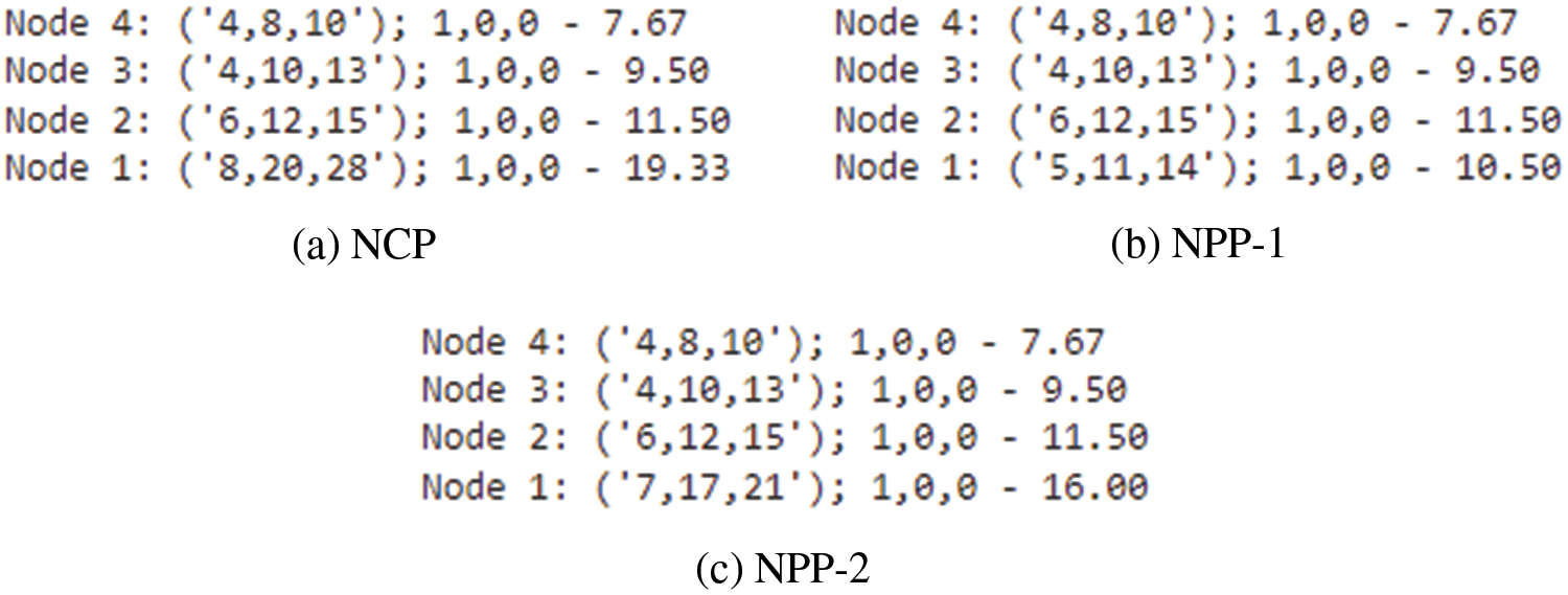
Figure 4: Case-II (F_kδ1>F¯kδ2)

Based on the condition (F_kδ1>F¯kδ2). The obtained NCPL is <(8,20,28);1,0,0> and the NCP of 1-3-4-5 yields a project completion time of SCCPL with 19.33 days, as observed in Fig. 4a. Alternative NPP-1 and NPP-2 have been explored in Figs. 4b and 4c, respectively, similar to case I of Example 4.2.1. However, there is a change in the NCCPL, having 10.50 days and 16.00 days, and their respective NCPLs are <(5,11,14);1,0,0> and <(7,17,21);1,0,0)>.

Example 4.2.3. Case-III: If the DM chooses the hybrid approach condition as (F_kδ1>F¯kδ2), (F_kδ1<F¯kδ2), (F_kδ1=F¯kδ2)

Solution: Similarly, implementing the algorithmic approach from steps 1 to 9, the obtained lower and upper bounds as: F_121=1, F¯122=2, F_131=4, F¯132=3, F_141=1, F¯142=1, F_241=3, F¯242=2, F_341=1, F¯342=2, F_451=5, F¯452=3 to satisfy the Eq. (3.2) is determined in Table 3 as follows:

Upon the analysis using three hybrid case-III (F_kδ1>F¯kδ2),(F_kδ1<F¯kδ2) and, (F_kδ1=F¯kδ2) by satisfying the Eq. (3.2), this integrated approach performs a balanced view of precise, conservative, and optimum estimations, and the results are defined in Figs. 5a–5c.

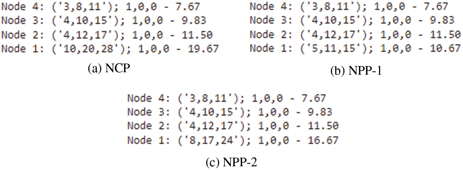
Figure 5: Case-III (F_kδ1>F¯kδ2),(F_kδ1<F¯kδ2),(F_kδ1=F¯kδ2)

For case-III, the NCPL is <(10,20,28);1,0,0> from the NCP of 1→3→4→5, with the obtained completion time of SCCPL being 19.67 days from Fig. 5a. The NPP-1 and NPP-2 are derived similarly to Examples 4.1 and 4.2 but with slight changes in the completion times of SCCPL, which are 10.67 days and 16.67 days, along with the NCPL as <(5,11,15);1,0,0> and <(8,17,24);1,0,0> defined in Figs. 5b and 5c. The CP and NPP from the three distinct cases are depicted in Fig. 6.

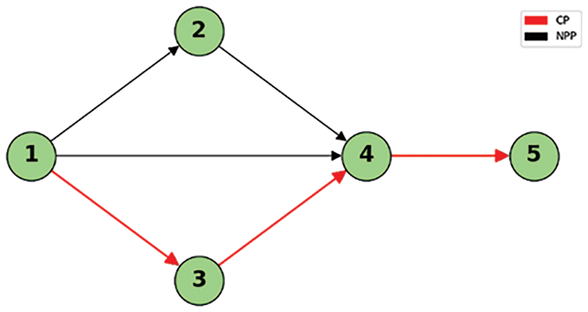
Figure 6: CP and NPP

Synthesizing the neutrosophic decision-making parameter involving three distinct cases to illustrate the complexity of project uncertainty and equivalence. The condition (F_kδ1<F¯kδ2) suggests an underestimation of activity durations, generally leading to optimistic project timelines. while (F_kδ1>F¯kδ2) indicating an overestimation, suggesting risk aversion. The hybrid approach combines three conditions (F_kδ1>F¯kδ2),(F_kδ1<F¯kδ2) and (F_kδ1=F¯kδ2), includes both conservative and optimistic estimates alongside precise forecasts, offering a well-rounded view that might deliver the practical unpredictable project settings. Notably, convergence proves the neutrosophic approach compatibility and liability over the initial study of CCPP and FCPP. The analysis is detailed in Table 4 covering the discussion of obtained CCPL from the existing literature of FCPP [40], by calculating CCPL, FCP, FCPL and, our proposed method in neutrosophic environment for Example 4.2. Further, the discussion of NCP and NPP of Example 4.2 is referred in Table 5 and the study representation of classical, fuzzy, and neutrosophic findings with visualization is provided in Fig. 7.

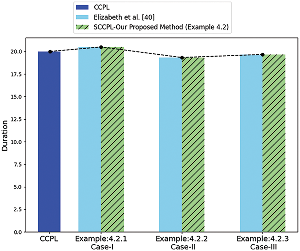
Figure 7: Comparison of classical, fuzzy, and neutrosophic (ref Table 4)

4.3 Analysis of Neutrosophic Path Lengths Under Varied Degrees

Example 4.3. Within this framework, the study now advances by exploring neutrosophic with varied degrees of uncertainty. From the previous Example 4.2, the study outlines TrSVN with (dpN,epN,fpN) parameters as (1,0,0) to the network for analyzing its behavior. The subsequent new problem, presented in Example 4.2, extends the investigation to incorporate variations in the (dpN,epN,fpN) parameters that are presented in Table 6, for evaluating the network’s responsiveness to dynamic changes within the environment.

Solution: From Table 6, the proposed algorithm from steps 1 to 9 evaluates the result outcomes of NCPP. It illustrates different neutrosophic conditions by varying uncertainty parameters; the obtained SCCPL is 17.36 days, when illustrated the condition F_kδ1<F¯kδ2 having NCPL of ⟨(13,20,30);0.85,0.16,0.15⟩, when F_kδ1>F¯kδ2 having ⟨(8,20,28);0.85,0.16,0.15⟩ of 16.37 days, and the condition for the hybrid approach of F_kδ1>F¯kδ2,F_kδ1<F¯kδ2, F_kδ1=F¯kδ2 having NCPL ⟨(10,20,28);0.85,0.16,0.15⟩ having 16.65 days, where the NCP remains same for three distinct cases as 1→3→4→5. The study exhibits a marked improvement over the traditional CCPP approach, which estimates a static 20 days, because FCPP cannot be resolved within the neutrosophic context, as highlighted in Table 7, and the discussion of other possible paths is provided in Table 8.

The comparison between Example 4.2 and Example 4.3 involving the study results having the same NCP as 1→3→4→5 using three different cases with their respective duration time is illustrated in Fig. 8, even though FCPP is part of the discussion but does not solve our proposed neutrosophic model and further for brief overview of NCP, logical comparisons are detailed in Table 9. A more robust adaptability and precision of NCPP in project management under varying conditions of uncertainty underscores the potential to enhance better decision-making by incorporating a broader range of probabilistic outcomes, which ultimately leads to robust planning and execution strategies.

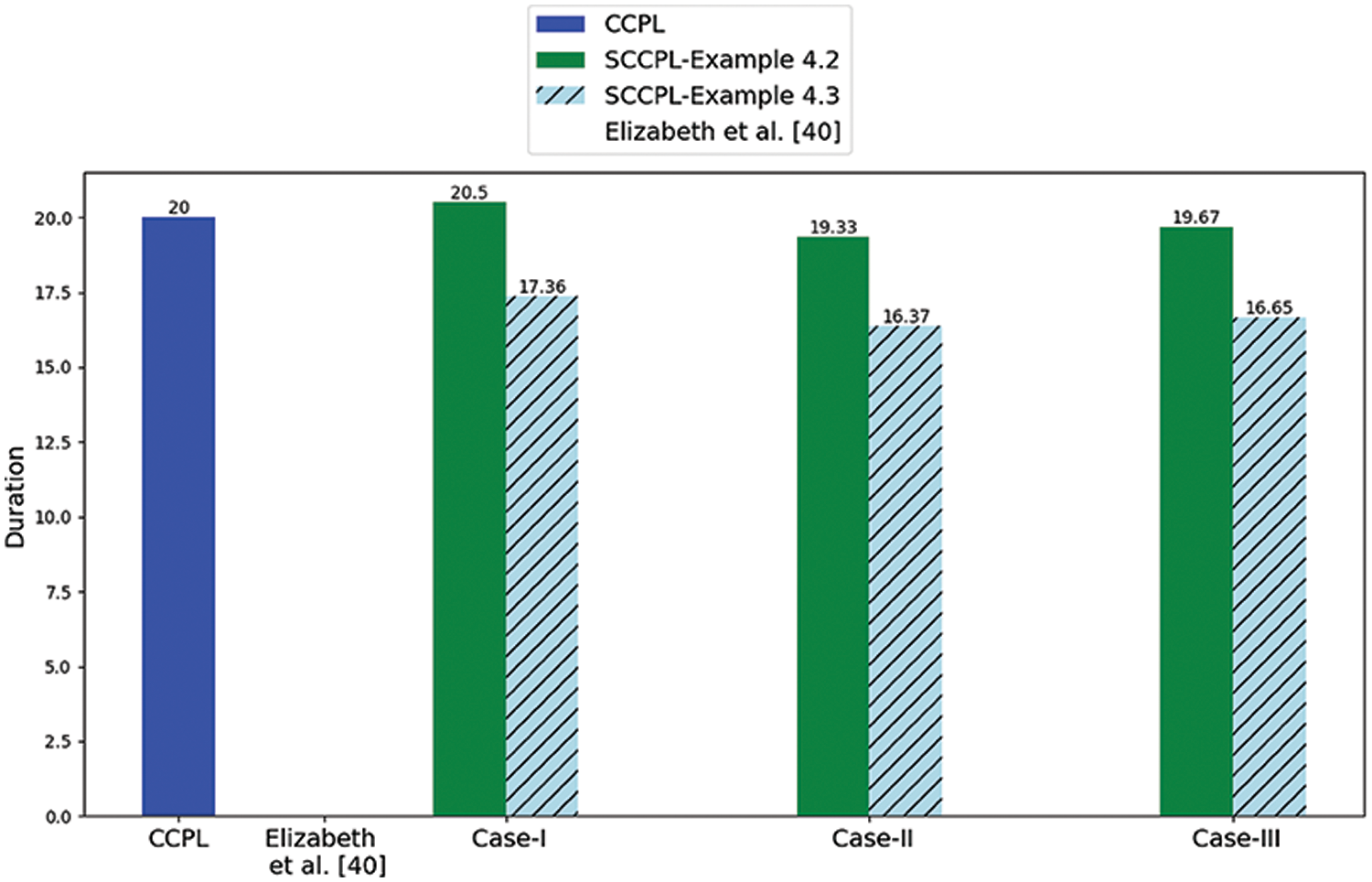
Figure 8: Comparison of neutrosophic with varying conditions against existing models (ref Tables 7 and 4)

A comparison of NCPP with both conventional CCPP and FCCPP was the primary emphasis of Examples 4.2 and 4.3. More conventional systems tend to simplify or ignore the inherent uncertainties in project management activities; the main goal was to evaluate NCPP’s ability to accommodate and dynamically adapt to these uncertainties.

5  Conclusion

Our study proposes a structured NCPP model that integrates into project management networks. This dynamic method’s adaptive algorithm updates project uncertainty dynamically. By leveraging the capabilities of TrSVNN, the NCPP facilitates a refined measurement of uncertainty that plays a crucial role in the field of complex projects. Using NCPP in three different situations gives a more varied result while keeping the same NCP as 1→3→4→5. This results in an SCCPL duration time of 20.50 days for condition (F_kδ1<F¯kδ2) with NCPL ⟨(13,20,30);1,0,0⟩, 19.33 days for condition (F_kδ1>F¯kδ2) having NCPL as ⟨(8,20,28);1,0,0⟩, and 19.67 for the three integrated situations of (F_kδ1>F¯kδ2),(F_kδ1<F¯kδ2), and (F_kδ1=F¯kδ2) having NCPL as ⟨(10,20,28);1,0,0⟩, while keeping the uniform approach in Example 4.2. Later, the study refines to varied deviations; the obtained SCCPL is 17.36, having NCPL as ⟨(13,20,30);0.85,0.16,0.15⟩, and SCCPL is 16.37 for condition (F_kδ1>F¯kδ2) and 16.65 for hybrid approach (F_kδ1>F¯kδ2),(F_kδ1<F¯kδ2), (F_kδ1=F¯kδ2), having NCPL as ⟨(8,20,28);0.85,0.16,0.15⟩ and ⟨(10,20,28);0.85,0.16,0.15⟩ with varying conditions in Example 4.3. The results emphasize the study’s presentation that NCPP has superior analysis that outperforms and effectively compares existing methodologies such as CCPP and FCPP for enhancing project uncertainty management. Employing an innovative methodology and utilizing Python for computational implementation significantly enhances the field of research. The current body of research on the application of CPP to various real-world scenarios is limited, suggesting a potential lack of research in this area. In the future, the investigation of using CPP may vary widely by studying different unpredictable circumstances.

Acknowledgement: The authors express their sincere gratitude to the reviewers and the chief-editor for their valuable insights and suggestions, which significantly enhanced the quality and depth of our paper.

Funding Statement: The authors received no specific funding for this study.

Author Contributions: The authors confirm contribution to the paper as follows: study conception and design: Navya Pratyusha M., Kumar R.; analysis and interpretation of results: Navya Pratyusha M., Kumar R.; draft manuscript preparation: Navya Pratyusha M. The authors reviewed the results and approved the final version of the manuscript.

Availability of Data and Materials: All the data contained in this study from the necessary sources can potentially access or by getting in touch with the paper’s corresponding author.

Conflicts of Interest: The authors declare that they have no conflicts of interest to report regarding the present study.

References

1. Idama A. Operational research applications for management decision-making. Yola, Nigeria: Paracelete Publishers; 1999. [Google Scholar]

2. Mazlum M, Guneri AF. Cpm, pert and project management with fuzzy logic technique and implementation on a business. Procedia-Social and Behav Sci. 2015;210:348–57. doi:10.1016/j.sbspro.2015.11.378. [Google Scholar] [CrossRef]

3. Kelley JE, Walker MR. Critical-path planning and scheduling. In: Eastern Joint IRE-AIEE-ACM Computer Conference; 1959; New York, USA. doi:10.1145/1460299.1460318. [Google Scholar] [CrossRef]

4. Kholil M, Alfa BN, Hariadi M. Scheduling of house development projects with CPM and PERT method for time efficiency (case study: house type 36). IOP Conf Series: Earth and Environ Sci. 2018;140(1):1–8. doi:10.1088/1755-1315/140/1/012010. [Google Scholar] [CrossRef]

5. Malcolm DG, Roseboom JH, Clark CE, Fazar W. Application of a technique for research and development program evaluation. Operat Res. 1959;7(5):646–69. doi:10.1287/opre.7.5.646 [Google Scholar] [CrossRef]

6. Akpan NP, Agadaga GO. Modelling building renovation using pert. Asian Res J Math. 2020;16(4):25–38. doi:10.9734/arjom/2020/v16i430184. [Google Scholar] [CrossRef]

7. Hajdu M, Bokor O. The effects of different activity distributions on project duration in pert networks. Procedia-Social and Behav Sci. 2014;119(19):766–75. doi:10.1016/j.sbspro.2014.03.086. [Google Scholar] [CrossRef]

8. Shah A. PERT vs. CPM: a cross review analysis. Int J Social Impact. 2021;6(1):33–43. [Google Scholar]

9. Habibi F, Birgani OT, Koppelaar H, Radenovic S. Using fuzzy logic to improve the project time and cost estimation based on project evaluation and review technique (PERT). J Project Manag. 2018;3(4):183–96. doi:10.5267/j.jpm.2018.4.002. [Google Scholar] [CrossRef]

10. Yuliarty P, Novia Nila S, Anggraini R. Construction service project scheduling analysis using critical path method (CPMproject evaluation and review technique (PERT). Int J Innov Sci Res Technol. 2021;6(2):477–80. [Google Scholar]

11. Zadeh LA. Fuzzy sets. Inf Control. 1965;8(3):338–53. doi:10.1016/S0019-9958(65)90241-X. [Google Scholar] [CrossRef]

12. Wan SP, Dong JY, Chen SM. A novel intuitionistic fuzzy best-worst method for group decision making with intuitionistic fuzzy preference relations. Inf Sci. 2024;666(6):120404. doi:10.1016/j.ins.2024.120404. [Google Scholar] [CrossRef]

13. Yen KK, Ghoshray S, Roig G. A linear regression model using triangular fuzzy number coefficients. Fuzzy Sets Syst. 1999;106(2):167–77. doi:10.1016/S0165-0114(97)00269-8. [Google Scholar] [CrossRef]

14. Rezvani S. Ranking method of trapezoidal intuitionistic fuzzy numbers. Annals of Fuzzy Math Inform. 2013;5(3):515–23. [Google Scholar]

15. Rameshan N, Dinagar DS. A method for finding critical path with symmetric octagonal intuitionistic fuzzy numbers. Adv Math: Sci J. 2020;9(11):9273–86. [Google Scholar]