A High-Accuracy Curve Boundary Recognition Method Based on the Lattice Boltzmann Method and Immersed Moving Boundary Method

Nomenclature

1  Introduction

In various fields, including aircraft engineering [1–3], ocean engineering [4–6], construction engineering [7,8], geological engineering [9,10], and others, coupled computational techniques such as the LBM and IMB are employed to simulate the impact of two-dimensional complex curved solid boundaries on the flow field and facilitates the extraction of information about the flow field within the computational domain, simplifying numerous three-dimensional fluid-structure coupling problems, which effectively diminishes a substantial amount of computational complexity. Examples of such problems include wing flow, ship flow, and bridge pier flow, among others.

There are two popular LBM fluid-solid coupling methods: one is based on the IBM [11,12], defined as IBM-VC in this study, which corrects the velocity of the solid boundary to meet the slip-free boundary condition. IBM-VC can identify complex curve boundaries through boundary node velocity interpolation. IBM-VC was gradually developed, including multiphase flow coupling, moving boundaries, computational efficiency, and others [13–16]. However, IBM-VC is prone to numerical instability [14,15]. Another alternative method is IMB [17], which introduces a solid node ratio covered by solid and weighting function in the additional collision term to calculate the solid boundary more accurately. IMB enables a smooth representation of the solid boundary contour, which many scholars have proved to be a method with high computational accuracy and stability [18–21]. However, when it comes to complex curve boundaries, the existing IMB still suffers from a significant problem related to curve boundaries. The algorithm proposed by Wang et al. [18] is not feasible for achieving custom curve boundary node detection by calculating the distance between nodes and the center of the circle or determining the area number of nodes on the circular particle. In addition, few scholars have investigated the coupling calculation of IMB at curve boundaries and multi-particle flow.

A curve boundary recognition method, IMB-CB, is introduced to promote IMB’s engineering applicability. This IMB-CB, based on IMB, uses the intersection information matrix between the search box and the curve to determine the direction of the search box movement. Then, the search box is moved to identify boundary nodes, and the solid ratio of the boundary nodes is determined to correct the weighting function in the LBM collision operator, achieving accurate recognition of custom curve boundaries. In addition, the study involves error analysis of curve boundary recognition, the influence of grid size on Poiseuille flow, numerical simulation of flow in custom curve boundaries, and flow patterns around a NACA0012 airfoil with scattered data. The calculated results are systematically compared to those obtained through IBM-VC to assess the precision and reliability of the algorithm. Considering the application of IMB-CB in moving boundaries, numerical simulations were conducted for multi-moving particle flow in curved pipelines.

2  Method

2.1 Basic Theory of IMB-CB

In the Lattice Boltzmann Method, when the system is subjected to body forces Fi, and when the nodes of the lattice elements collide, the LBE [22] is described as follows:

fi(x+ciΔt,t+Δt)−fi(x,t)=Ω(fi)+Fi⋅Δt,(1)

where x is the spatial coordinates of a lattice element node; t is the time, c is the velocity of the lattice element node; f(x, c, t) is the velocity distribution function; Ω(fi) is the collision operator that influences the rate of change of state of lattice element nodes before and after the collision; i is the direction of discretization of lattice element velocity.

The BGK [23] model has better computational efficiency and is commonly used in lattice Boltzmann methods compared to the MRT model [24–26]. The BGK collision operator is expressed as follows:

Ω(fi)=−Δtτ[fi(x,t)−fieq(ρ(x,t),u(x,t))],(2)

where fieq(ρ(x,t),u(x,t)) is the function of equilibrium distribution in i direction; τ is the relaxation time related to fluid viscosity which is defined as υ=Δx2(τ−0.5)/(3Δt) and fieq(ρ(x,t),u(x,t)) is described as follows:

fieq(ρ(x,t),u(x,t))=ωiρ(x,t)[1+ci⋅ucs2+12(ci⋅u)2cs4−12u2cs2],(3)

where ωi is the weight factor in different speed directions; ρ(x,t) is the macroscopic fluid density; u is the macroscopic fluid velocity; ci is the lattice velocity vector given by ci=|ci|ci, |ci| represents a lattice velocity scalar; ci is the lattice velocity unit vector; cs is the lattice sound velocity given by cs=|ci|/3 related to the lattice length h and time step of the grid Δt, given by |ci|=h/Δt.

In IMB, as proposed by Noble et al. [17], a modified LBE is derived by incorporating an additional collision operator and a weighting function into the pre-existing collision operator. The LBE augmented with additional collision operators can make it equivalent to LBE with body forces. This equivalence can be represented as follows [27]:

fi(x+ciΔt,t+Δt)−fi(x,t)=−Δtτ[fi(x,t)−fieq(ρ,u)]+BsΔt[fieq(ρ,Us)−fieq(ρ,u)]⋅Δt.(4)

Eq. (4) can be understood as the body forces Fi=Bs[fieq(ρ,Us)−fieq(ρ,u)]/Δt in Eq. (1), where Bs is the weighting function at the node s regarding the solid ratio of the node, given by

Bs=εs(τ/Δt−0.5)(1−εs)+(τ/Δt−0.5).(5)

The solid ratio εs is expressed by drawing a square with a side length of lattice size h at a node and calculating the ratio of the area A of the intersection between the square and the interior of the solid to the area of the square. The solid ratio εs is described by εs=A/h2, when the node is an external fluid node, εs=0; when the node is an internal solid node, εs=1.

The hydrodynamic force and torque exerted on the solid particles, which cover n nodes and are subjected to the fluid, can be mathematically expressed as follows:

Ff=|c|h[∑n(Bs,n∑iΩs,ic−i)],(6)

Tf=|c|h[∑n(xn−xc)×(Bs,n∑iΩs,ic−i)].(7)

where Ωs,i is a collision operator based on the bounce rule for the non-equilibrium part, provided as follows:

Ωs,i=fieq(ρ, Us)−fieq(ρ, u)+Δtτ[fieq(ρ, u)−fi(x, t)],(8)

where Us is the motion velocity vector at particle node s.

In the LBM, the lattice unit nodes are modeled with multi-dimensional and multi-velocity direction models, such as the commonly-used DnQm model, where Dn is n dimensions and Qm represents m velocity directions. This study focuses on the algorithm for recognizing two-dimensional curved boundaries, with particular emphasis on the D2Q9 model selected as the focal point for this investigation, as illustrated in Fig. 1. The fluid computational domain in this model is discretized into a grid with a grid edge length of h. Grid unit nodes, with nine velocity directions designated as 0–8, undergo collision and migration along their respective velocity directions. The velocity vector in the D2Q9 model is expressed by

Figure 1: D2Q9 model

ci={(0,0),i=0(cos⁡[(i−1)π2],sin⁡[(i−1)π2]),i=1⋯42(cos⁡[(i−1)π2+π4],sin⁡[(i−1)π2+π4]),i=5⋯8.(9)

For the D2Q9 model, the macro fluid density ρ and macro fluid velocity u can be calculated from the velocity distribution function, given by

ρ=∑i=08fi,(10)

ρu=∑i=08fici.(11)

The theoretical knowledge of IBM-VC based on second-order Lagrangian interpolation for velocity correction can be found in the literature [14]. This study mainly focuses on IMB-CB and compares the numerical simulation results obtained by IMB-CB to IBM-VC.

As the LBM operates within its unique unit system, simulating real-world physical phenomena requires converting actual physical quantities into LBM lattice units. This conversion process is known as establishing dimensionless physical parameters.

Assuming in a computational domain of L×H, which corresponds to the lattice domain of n∗×m∗ in LBM (represented by the actual physical unit without a * sign and the LBM lattice unit with a * sign), and the actual fluid viscosity is v. Initially, the computational domain is discretized. The unit length of the lattice is Δx=1 and the unit time length is Δt=1, resulting in the lattice velocity ck=Δx/Δt. If the characteristic length of L is discretized into n lattice units, the actual length depicted by a single lattice is L/n. The selection of the number of grids is pivotal for the accuracy and efficiency of numerical simulation. If the number of grids is too small, divergence and inaccuracy may ensue. In contrast, an excessive number of grids can lead to diminished computational efficiency. Hence, the length conversion coefficient is obtained as follows: Cle=L/n. In the application of LBM, the macroscopic Reynolds number of the fluid is equal to the LBM Reynolds number, i.e., Re=uL/v=u∗n∗/v∗, where u is the average velocity of the flow field. For the BGK model, LBM can simulate incompressible fluid flow under low Mach number (Ma) conditions and with little density variation, while high Ma can lead to computational instability. The Ma is defined as Ma=u∗/cs.

Design with Ma as the constraint condition to obtain a stable lattice conversion coefficient. Set a low Ma to derive the lattice velocity u∗. When simulating high Reynolds number problems, either increase the number of grids or reduce the kinematic viscosity. Then, the velocity conversion coefficient is obtained as Cu=Cle/Ct=u/u∗, and the time conversion coefficient is determined as Ct=Cle/Cu. The viscosity conversion coefficient is obtained from the viscosity unit dimension m2/s as Cυ=Cle2/Ct. Finally, the lattice viscosity is obtained as υ∗=υ/Cυ. Again, the relaxation time in the lattice Boltzmann equation for BGK approximation τ=υ∗cs2Δt/Δx2+0.5 is calculated. The density conversion coefficient is Cρ=ρ/ρ∗, where the fluid density in the lattice domain is generally considered ρ∗=1.

By adhering to the dimensionless steps outlined for the parameters above, accurate numerical simulations corresponding to real physical problems can be attained, thus ensuring numerical stability.

2.2 Curve Boundary Recognition Algorithm of IMB-CB

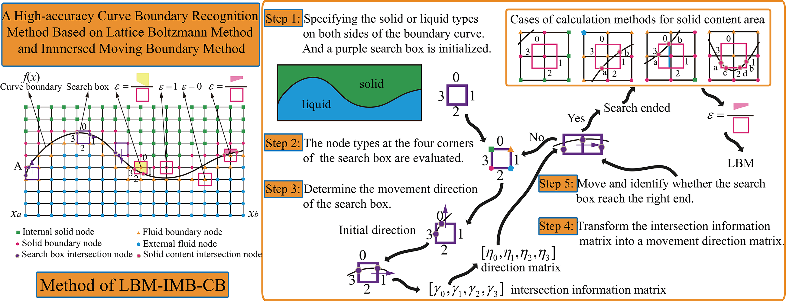
Fig. 2 indicates that the schematic diagram of the curve boundary model encompasses internal solid nodes, solid boundary nodes, fluid boundary nodes, and external fluid nodes. For the black boundary curve f(x) with a known definition domain x∈[xa, xb], the steps for curve boundary recognition are as follows:

Figure 2: Schematic diagram of curve boundary recognition method model

(1) The initial step involves specifying the solid or liquid types on both sides of the boundary curve. It is assumed that the nodes in the computational domain above the function f(x) are solids, while nodes below the function f(x) are liquids. Then, a purple search box is initialized with the upper adjacent node A, located at the point (xa, f(xa)), in the left corner. This search box is defined by its upper, right, bottom, and left edges, numbered as 0, 1, 2, and 3, respectively.

(2) Subsequently, the node types at the four corners of the search box are evaluated. If yj>f(xi) at the corner node (xi, yj) of the search box, it is marked as a solid boundary node; conversely, if yj<f(xi) at the corner node (xi, yj) of the search box, it is identified as a fluid boundary node.

(3) In addition, to determine the movement direction of the search box, the first step is to establish its initial direction of movement. Firstly, it is necessary to determine whether the curve boundary f(x) intersects with edges 0, 1, 2, and 3 of the search box and represent this intersection information in matrix form [γ0, γ1, γ2, γ3]. If an intersection occurs, γs=1; otherwise, γs=0, where s=0, 1, 2, 3.

(4) To transform the intersection information matrix into a movement direction matrix [η0, η1, η2, η3], where the edge with ηs=1 represents a specific direction of the search box’s movement, it is essential to identify whether it is the first cycle. If it is, the elements of the intersection information γs corresponding to the left boundary of the function definition domain are assigned a value of 0. If it is not the first cycle, γs¯ in the intersection information matrix that corresponds to the edge opposite to the movement direction ηs of the previous cycle is assigned a value of 0, where s¯=2, 3, 0, 1. In contrast, the value of other edges is assigned γs=ηs (For example, if the direction of the search box’s movement in the previous step is 0 edge, the intersection information of the opposite two edges will be assigned as γ2=0). Thus, the intersection information matrix [γ0, γ1, γ2, γ3] is transformed into the movement direction matrix [η0, η1, η2, η3] of the search box.

(5) Finally, the search box should be repositioned based on the direction matrix [η0, η1, η2, η3] and identify whether the search box reaches the right end of the definition field. If it is, the recognition of this node is complete. If not, the algorithm returns to step (2).

For the schematic diagram of the curve boundary recognition method model depicted in Fig. 2, the leftmost search box corresponds to the first cycle, whose intersection information matrix is [1, 0, 0, 1]. Since the definition domain x∈[xa, xb] of the function f(x) spans from left to right in the lattice domain, the three edges in the search box are assigned a value of 0 in the corresponding positions of the intersection information matrix, resulting in the direction matrix [1, 0, 0, 0]. As a result, the first movement direction is upward. After moving the search box one lattice unit based on the direction matrix, the node coordinates of the search box are updated, and the node type is determined. The search box is then moved along the new direction matrix [η0, η1, η2, η3] again, and the node type and intersection information matrix are determined. This cycle process continues until the abscissa of the node on the right side of the search box exceeds xb. At that point, the curve boundary recognition algorithm ends.

If the boundary of the given curve is not a continuous function f(x) but a scattered data (xj, yj) of the curve, linear interpolation can be utilized when calculating on the f(xi) of corner node (xi, yj) of the search box, given by

f(xi)=(yj+1−yj)(xi−xj)xj+1−xj+yj,(12)

where xj≤xi≤xj+1.

Using search boxes to traverse curve boundaries and ascertain the solid or fluid boundary nodes can increase the algorithm’s time complexity. This study explores the computational complexity involved in identifying curve boundaries in IMB-CB and its computational efficiency. The computational complexity of this curve boundary identification algorithm is linear and is described as follows:

O(n)=∫xaxb1+f′(x)2dx/h,(13)

where f′(x) is the derivative of the curve function and h is the lattice size.

If the method proposed by Wang et al. [28] in 2017 for identifying nodes of granular fluid boundaries and solid boundaries, respectively, is improved based on the method in this study to be a customized curve boundary identification method, the time complexity is expressed as follows:

O(n)=2∫xaxb1+f′(x)2dx/h.(14)

The computational method in this study will reduce the computational complexity by half compared to this kind.

After identifying the node types of the curve boundary, it is necessary to use εs=A/h2 to calculate the solid ratio of these nodes. When the node type is an external fluid node, A=0, and when the node type is an internal solid node, A=1. The calculation of solid ratio at solid boundary nodes and fluid boundary nodes involves dividing the intersection area between the node area box (with a side length of h) and the interior of the solid by the area of the node area box, as depicted in Fig. 2. Assuming that nodes in the computational domain below the function f(x) are solids, while nodes above the function f(x) are fluid. The edges of the node area box are denoted by 0, 1, 2, and 3, corresponding to the edges of the search box, and the intersection information matrix [γ0, γ1, γ2, γ3] of the node area is also obtained. The intersection points of a, b, c, and d intersect the curve boundary and the node area box. Due to various information matrices and calculation methods associated with different calculation cases, the potential cases are categorized into four distinct cases, as depicted in Fig. 3. These cases represent the different calculation methods applied to the solid area of the boundary nodes. Among them, the symbols assigned to the nodes bear the same significance as those in Fig. 2. The cases, intersection information matrix, and area calculation method are summarized in Table 1, which presents the different calculation methods for the solid area of curve boundary nodes. The three-point Gaussian Legendre formula is utilized in this algorithm to integrate the curve boundary function.

Figure 3: Cases of calculation methods for the solid content area of curve boundary

In Fig. 3a case 1, if the intersection matrix consists entirely of 0, and if the node is situated within the solid region, A=1; if the node lies within the liquid region, A=0. In Fig. 3b case 2, if γ0=0, and two among (γ1, γ2, γ3) are equal to 1, the area is determined using the integration to compute the surface area. In Fig. 3c case 3, if γ0=1, and one among (γ1, γ2, γ3) is equal to 1, the sum of the trapezoidal area of the curved edge and the area of the divided small rectangle are calculated using the integration. The intersection area between the node area box and the curve boundary will be obtained. If three among (γ0, γ1, γ2, γ3) are equal to 1, and if the node is situated within the solid region, A=1; if the node lies within the liquid region, A=0. After calculating the intersection area between solid boundary nodes and fluid boundary nodes, the solid ratio is computed using εs=A/h2. If a node in the computational domain is solid above the function and liquid below the function, and the area enclosed by the solid is obtained by subtracting the intersection area from the node area, then the solid ratio is described as follows: εs=(h2−A)/h2.

In order to improve the calculation accuracy of the area A of a curved trapezoid, the Gauss-Legendre formula can be used, given by

A=∫abf(x)dx≈b−a2∑i=1Nwif(a+b−a2(1+ξi))(15)

where f(x) is the curve boundary function; a and b are the lower and upper integral limits, respectively; ξi is the Gaussian point abscissa; N is the order; wi is the weight factors with i=1, 2,⋯,N.

Table 2 presents the parameters of three area algorithms. By summing up the node areas covered by all solid particles and analyzing the error in their original areas, the resulting error can be expressed as follows:

error=|Ssolid−∑nASsolid|×100%(16)

where Ssolid is the actual area of solid particles; Ssolid=πr2; r is the radius of the particle.

A solid particle with coordinates (0.1, 0.1 m) and radius r=0.05m is placed within a calculation domain with a length of L=0.2 m and a height of H=0.2 m. The solid ratio error obtained by the three area computing formulas for the particle is calculated using the IMB method at different lattice sizes. Fig. 4 depicts the relationship between the solid ratio error and the number of particle diameter grids. It illustrates that when using the first-order Newton-Cotes formula (1-N-C) for calculation, the maximum error is 0.69% when the number of particle diameter lattices is 10. When employing the two-point Gauss-Legendre formula (2-G-L), the maximum error is 0.075%. Similarly, when utilizing the three-point Gauss-Legendre formula (3-G-L), the maximum error is 0.05%. The solid ratio error values for these three calculation methods gradually decrease as the number of particle diameter lattices increases. The first-order Newton-Cotes formula (1-N-C) generally exhibits higher error values than the other two calculation methods, whereas the three-point Gauss-Legendre formula (3-G-L) yields the smallest error value. Hence, this study selects the three-point Gauss-Legendre formula (3-G-L) as the preferred calculation method for solid ratio.

Figure 4: Curve of solid ratio error and number dn of particle diameter lattices

3  Numerical Simulation Results

3.1 Recognition of Custom Curve Boundary

In order to validate the feasibility and accuracy of the curve boundary recognition method and the solid ratio algorithm, an assumption is made regarding the presence of a curve boundary defined by a function f(x)=0.5cos(2x)+0.8 within a computational domain characterized by a length of L=5 m and a height of H=1.5 m. Under this scenario, nodes positioned above the function are considered solid, while those located below the function are deemed fluid within the computational domain. This study investigates the influence of lattice size h on curved boundary recognition by utilizing varying lattice sizes. Specifically, three different values for the number of lattices, denoted as Xn, in the X-direction, are considered: 50, 100, and 500, respectively. The length conversion coefficients are Cle=L/Xn=0.1 m, Cle=0.05 m, and Cle=0.01 m, respectively. As proposed in this study, the curve boundary recognition algorithm is employed to compute solid ratios within the computational domain. The resulting data is then graphically depicted in Fig. 5, where Fig. 5a corresponds to Xn=50, Fig. 5b corresponds to Xn=100, and Fig. 5c corresponds to Xn=500.

Figure 5: Solid ratio cloud map of curve boundary under different lattice numbers

Fig. 5 indicates that the upper segment of the boundary curve exhibits a solid state, with a corresponding solid ratio of εs=1. In contrast, the lower segment of the boundary curve is characterized by a liquid state with a solid ratio of εs=0. As the number of lattices increases, the recognition accuracy of curve boundaries becomes more pronounced. Further examination of the enlarged boundary image in Fig. 5 reveals a high recognition accuracy of the curve boundary. In addition, the transition of the solid ratio value at the curve boundary from fluid to solid demonstrates a relatively uniform gradient pattern, substantiating the feasibility and accuracy of the curve boundary recognition method and solid ratio algorithm proposed in this study.

In order to further investigate the discrepancy between the identified curve boundary and the analytical solution of the curve equation, the curve information of the image is extracted through image processing of the solid ratio cloud map of the curve boundary at various grid resolutions, and the error is computed in comparison to the analytical solution. The specific procedures encompass the following:

Initially, Gaussian blur denoising is applied to the solid ratio cloud map, as derived from Fig. 5. The Sobel convolution kernel is utilized to compute the image’s gradient, and gradient amplitude and direction are determined based on the horizontal and vertical gradient components. Non-maximum suppression is subsequently employed on the gradient amplitude image. Following this, two thresholds are defined to categorize pixels into strong edges, weak edges, or non-edges. Using the connectivity of strong edge pixels, the ultimate edge line is constructed to yield a binary image of edge detection, as depicted in Fig. 5, where pixel values of 0 represent black, while 1 represents white.

Coordinate information is extracted from the white pixels in Fig. 6. Error bars are established at both ends by calculating the mean X-coordinate (xi, yiMean) from the maximum (xi, yiMax) and minimum coordinates (xi, yiMin) of the white pixels sharing the same X-coordinate. These error bars are subsequently compared with the analytical solution in the same xi, resulting in the acquisition of several curve boundary recognition points and a comparison diagram of the analytical solution under various lattice resolutions, as depicted in Fig. 6. The error between the mean coordinate (xi, yiMean) and the analytical solution yiA is computed using Eq. (17), yielding the error between the curve boundary identification points and the analytical solution for different grid resolutions.

Figure 6: Binary image of solid ratio cloud map under different lattice numbers

error=yiMean−yiAyiA×100%.(17)

Fig. 7 indicates that the curve boundary identification points closely align with the analytical solution. In addition, as the number of lattices increases, the range of error bars diminishes. When the number of lattices reaches Xn=50, the error approximates −5.7%∼+6.2%, signifying a dispe- rsion; at Xn=100 lattices, the error decreases to approximately −2.8%∼+2.4%, representing a relatively modest level of dispersion; and at Xn=500 lattices, the error further reduces to close to −1.8%∼+0.8%, indicating the least degree of dispersion. These results are compelling evidence that the error in curve boundary recognition proposed in this article is exceedingly small. In addition, the reduction in error as the number of lattices increases underscores the algorithm’s remarkable accuracy in identifying custom curves.

Figure 7: Comparison of curve boundary identification points and analytical solutions under different grid numbers

A point method was employed to evaluate the accuracy of calculating the solid ratio on grid points [27]. As illustrated in Fig. 8, for a grid with coordinates (300, 128) at Xn=500, a red box is drawn on the node to compute the solid ratio, which is then divided into nd×nd grids. Each small grid corresponds to a point in the point method, with the solid amount represented by the point being 1/nd. Hence, the solid ratio of the node calculated using the point method is denoted as follows:

Figure 8: Dot method for solid ratio

εd=Ndnd2Δx.(18)

where εd is the solid ratio of nodes calculated by the applied point method; Nd is the total number of points in a grid; Δx signifies the edge length of the solid ratio element box.

In the grid of (300, 128) depicted in Fig. 8, considering nd=10 and Δx=1, εd=50/100=0.5 utilizing the point method. In contrast, the solid ratio of (300128) calculated through IMB-CB was denoted as ε=0.492285, indicating that the algorithm proposed in this study offers higher accuracy and precision.

3.2 Poiseuille Flow within Custom Curve Boundaries under Different Lattice Sizes

Different lattice sizes were established based on the curved boundary outlined in Section 3.1 to investigate the algorithm’s adaptability to various grid sizes. Hence, the Poisson blade flow was introduced, and numerical simulation results were juxtaposed with the analytical solution. Set the same computational domain and boundary conditions as in Section 3.1. The fluid density is initialized as ρ=1000 kg/m3 and the fluid viscosity as υ=10−3m2/s. The left end of the domain is designated as the fluid inlet, while the right end serves as the outlet. A bounce rule of no-slip boundary condition is applied to the lower wall.

The entrance adopts Poiseuille flow, given by

u(0, y, t)=4Umy(H−y)/H2,(19)

where u(0, y, t) is the horizontal velocity at the coordinate point (0, y) at time t; y is the vertical coordinate point, y∈[0, H]; Um is the average velocity of the entrance Poiseuille flow.

The average velocity of the fluid is determined as follows:

U¯=23u(0, H/2, t).(20)

Then, the Zou-He velocity boundary condition is employed to set the velocity at the left entrance. The average velocity of the Poiseuille flow is set to Um=0.3 m/s at the left inlet of the rectangular channel. Set Ma=0.02887, then u∗=0.05. When Xn=50, the dimensional conversion coefficients between physical real units and LBM are: Cle=0.1 m, Cu=6 m/s, Ct=0.0167 s, Cυ=0.6 m2/s, Cρ=1000 kg/m3, and then the computational domain in LBM is n×m=50×15, υ∗=0.00167, τ=0.505. When Xn=100, the dimensional conversion coefficients between physical real units and LBM are: Cle=0.05 m, Cu=6 m/s, Ct=0.00833 s, Cυ=0.3 m2/s, Cρ=1000 kg/m3, and then the computational domain in LBM is n×m=100×30, υ∗=0.00333, τ=0.51. When Xn=500, the dimensional conversion coefficients between physical real units and LBM are: Cle=0.01 m, Cu=6 m/s, Ct=0.00167 s, Cυ=0.06 m2/s, Cρ=1000 kg/m3, and then the computational domain in LBM is n×m=500×150, υ∗=0.0167, τ=0.55. The calculated results are depicted in Fig. 9, illustrating the fluid velocity at the Y-direction nodes under various grid configurations. Fig. 9a displays the inlet velocity and Poiseuille flow analytical solution at X = 0, while Fig. 9b illustrates the velocity at X = 0.4 m at the onset of simulation 0.16667 s.

Figure 9: Y-direction node fluid velocity under different lattices

Fig. 9 indicates that when the inlet is positioned at X = 0, the outcome of Xn=500 closely aligns with the analytical solution of the Poiseuille flow. In contrast, the results obtained from Xn=50 and Xn=100 exhibit errors, with Xn=50 displaying the largest error, although it still accurately represents the Poiseuille flow. During the numerical simulation at 0.16667 s, significant changes were observed in the velocity at X = 0.4 m due to the influence of the curved boundary. The impact of different lattice sizes varied, attributed to the notable errors encountered when simulating LBM using coarse lattices. The curved boundary lies within the range of Y = 1.0 − 1.2 m. Despite the close velocity outcomes across different lattice sizes in this section, IMB-CB demonstrates close and high accuracy in identifying curved boundaries at Xn=50 and Xn=100. However, it is evident that employing too few lattices affects LBM. Thus, it remains imperative to select appropriate lattice sizes to ensure the reliability of numerical simulations.

3.3 Numerical Simulation of Flow in Custom Curve Boundary

The accuracy of the curve boundary recognition method based on IMB-CB is verified through the simulation of flow in custom curve boundary, compared to IBM-VC. Set the same computational domain and boundary conditions as in Section 3.2, when Xn=500.

A numerical simulation is performed to obtain the curve boundary simulation results shown in Fig. 10 using IMB-CB in this study. Figs. 10a and 10b respectively display the velocity cloud map and streamline diagram of the curved boundary. These simulation results correspond to the time t=12.5 s. It indicates that as the Poiseuille flow enters from the left end and passes through the narrow opening formed by the curved boundary, the fluid velocity experiences a significant increase, which aligns with the actual scenario. After traversing the narrow opening, the fluid enters a larger fluid domain, where the flow velocity decelerates and forms four vortices. This behavior resembles the phenomenon observed in a rectangular cavity driven by a top cover. As the fluid flows back into the slit, its velocity increases once again before eventually exiting through the outlet. Based on the phenomena above, it can be inferred that the LBM-IMB-CB is accurate and well-suited for numerical simulations involving complex curve boundaries and fluid-particle systems.

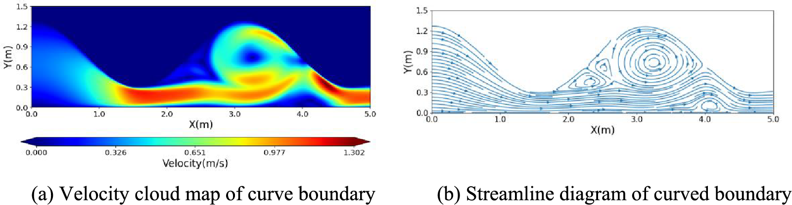
Figure 10: Simulation results at curve boundary IMB-CB

In IBM-VC, the same parameters as IMB-CB are set for numerical simulation, where Xn=500. Fig. 11 depicts the results at t=12.5 s obtained by employing the IBM-VC. It indicates that the simulation results are largely consistent with those obtained through IMB-CB in Fig. 10. Further comparison is conducted by examining the drag and lift coefficients (Cd and Cl) calculated using the IBM-VC. These coefficients offer valuable insights into the fluid forces and flow behavior associated with the flow around a cylinder within the context of fluid-structure coupling, given by

Figure 11: Simulation results at curve boundary of IBM-VC

{Cd=2FdρUm2LcCl=2FlρUm2Lc(21)

where Fd and Fl denote the fluid resistance and lift, respectively; ρ is the density of the fluid; D is the diameter of the cylinder; Lc is the characteristic length.

Fig. 12 illustrates a comparison graph of the Cd and Cl along the curve boundary. The results before 6.3 s are categorized as unstable flow areas, while those after 6.3 s are classified as stable. Within the stable flow region, IMB-CB yields an average Cd of 5.518 and an average Cl of 2.514. In contrast, IBM-VC produces an average Cd of 5.836 and an average Cl of 2.106. An analysis of the curve reveals that the average Cd and Cl at the curve boundary, computed using the two different methods, exhibit a high similarity. However, IMB-CB demonstrates superior numerical stability in the red dashed box of Fig. 12 compared to IBM-VC. Based on the above analysis, the IMB-CB accurately identifies custom curve boundaries while maintaining robust numerical stability.

Figure 12: Comparison curve of drag and lift coefficient at the curve boundary

3.4 Numerical Simulation of NACA0012 Airfoil Flow

This study conducts a flow validation using common NACA0012 airfoil data points at a Reynolds number (Re) of 500 to further validate the applicability of IMB-CB for scattered curve data. Since the Reynolds number in the fluid is determined as follows:

Re=ULcυ,(22)

where υ is the fluid viscosity.

The Original data points of NACA0012 airfoil are shown in Fig. 13, in which the characteristic length is the wing’s chord length, as Lc=1.0 m. The results are then compared with those of IBM-VC and those from previous research by Imamura et al. [29] using a generalized form of interpolation-supplemented LBM (GILBM). The computational domain is set to be L=3 m in length, H=1.0 m in height and the lattice length h=0.005 m. The fluid density is initialized as ρ=1000 kg/m3 and the fluid viscosity as υ=10−3m2/s. The maximum velocity of the Poiseuille flow is set to Um=0.5 m/s at the left inlet of the rectangular channel, resulting in a Reynolds number of Re=500 for the airfoil. The airfoil data points are shifted 0.5 m to the right and up, respectively, and the airfoil’s attack angle is set to 0, orienting the airfoil horizontally to the left of the middle of the computational domain. If Ma=0.02887, then u∗=0.05, and the dimensional conversion coefficient between physical real units and LBM is: Cle=0.005 m, Cu=10 m/s, Ct=0.0005 s, Cυ=0.05 m2/s, Cρ=1000 kg/m3, and the computational domain in LBM is n×m=600×200, υ∗=0.02, τ=0.56.

Figure 13: Original data points of NACA0012 airfoil

Utilizing the algorithm outlined in this study, curve boundary identification is executed on the scattered airfoil data of NACA0012, leading to the generation of a solid ratio cloud map, as depicted in Fig. 14. The resultant numerical simulation outcomes are subsequently juxtaposed with those derived from IBM-VC and compared with Cd and Cl findings reported by Imamura et al. [29]. Among them, the parameters taken by IBM-VC are the same as those of IMB-CB. The calculation results of velocity, vorticity, and streamline at 3.75 s, as displayed in Fig. 15, and the comparison results Cd featured in Fig. 16, are extracted for analysis. The average values of Cl and Cd from 2.0 to 3.75 s are displayed in Table 3. Table 3 also shows the results calculated by Imamura et al. using commercial software PowerFLOW and CFL3D.

Figure 14: Solid ratio cloud map of NACA0012 airfoil

Figure 15: Calculation results of NACA0012 airfoil flow

Figure 16: Comparison chart of drag coefficient around NACA0012 airfoil

Fig. 15 indicates that the Poiseuille flow, originating from the left end of the computational domain, symmetrically bypasses the NACA0012 airfoil, and the wake progressively elongates with time. A comparative assessment of the results obtained via the two methods reveals slight disparities in maximum velocity and vorticity values, while the remainder exhibit high similarity.

Turning attention to the drag coefficient outcomes displayed in Fig. 16, the numerical simulation experienced an unstable flow state during the initial 2.0 s but gradually transitioned into a stable flow state after 2.0 s, following the Poiseuille flow. The IMB-CB and IBM-VC methods employed in this study exhibit fluctuations around the average drag coefficient of 0.1725, a value reported in Imamura et al.’s study [29]. Nevertheless, upon closer examination of the enlarged graph covering the interval from 2.0 to 3.75 s in Fig. 16, IBM-VC manifests more pronounced numerical fluctuations, whereas the calculation results of IMB-CB demonstrate enhanced stability. The average calculation result of IMB-CB from 2.0 to 3.75 s stands at 0.1750, bearing an error of 1.45%, while the average calculation result of IBM-VC is 0.1637, accompanied by an error of −5.101%. The IMB-CB method delivers more precise results than IBM-VC. Due to the airfoil’s symmetry and a 0-degree angle of attack, the average lift coefficient closely aligns with 0. Upon inspecting the average lift coefficient values in Table 2, the average value of the IMB-CB method’s calculation results in this study, ranging from 2.0 to 3.75 s, closely approximates 1.6538×10−13, with an error value of 0.6538×10−13 when compared to Imamura et al.’s study [29]. In contrast, the calculation results of IBM-VC exhibit an average value of 2.8298×10−3 and an error value of 2.8298×10−3.

In summary, the IMB-CB proves proficient in accurately delineating curve boundaries for continuous functions and scattered data, yielding stable numerical calculation results of high precision.

3.5 Multi-Particle Flow in the Custom Complex Curved Pipeline

In order to verify the applicability of IMB-CB in moving boundaries, the discrete element method (DEM) is introduced in this study for calculating the motion of multiple particles within the LBM-IMB-CB framework, aiming to numerically simulate and assess the reliability of IMB-CB [30].

The coupling method flowchart of LBM-DEM-IMB is shown in Fig. 17. First, the fluid domain is discretized into a lattice domain by LBM, and the fluid and particle information are initialized. IMB recognizes custom complex curved boundaries and calculates the weighting function of solid ratio. Then, IMB recognizes particle boundaries and calculates the weighting function of the solid ratio. In addition, collision and migration of LBM distribution functions and update the grid domain’s velocity, density, and vorticity. In addition, the particle fluid force is calculated by IMB. The force of the particles, such as collision forces, gravity, buoyancy, torque, and others, is then calculated. The equations of motion of particles are calculated, and the coordinates of particles are updated accordingly. Judge whether the maximum DEM iteration step is reached. If not, return to continue calculating the particle force and equations of motion. However, if the maximum DEM iteration step is reached, the process proceeds to the next LBM iteration step. Similarly, evaluate whether the maximum LBM iteration step is reached. If not, the calculation proceeds to the IMB step for particle boundary determination. However, if the maximum LBM iteration step is reached, the calculation results are outputted, and the process concludes.

Figure 17: LBM-DEM-IMB-CB method flowchart

The discrete element soft sphere particle contact model in the DEM is equated with the discrete element spring damping dynamic model. When collisions between particles occur, the constitutive model is utilized to solve the contact force. Subsequently, the motion laws of the particles are determined by solving the Lagrange equations, which are given by

md2xdt2=Fn+Fs+Ff+mg,(23)

Jd2θdt2=Tc+Tf,(24)

where m and J are the mass and the moment of inertia of particles, respectively; x and θ are the displacement and the angular displacement of the particles, respectively; Fn, Fs, and Tc are the normal contact force, tangential contact force, and torque acting on particles or between particles and boundaries; Ff and Tf are the hydrodynamic force and torque of fluid on particles.

The normal and tangential contact forces between particles are determined by [31,32]

Fn,i,j=(knUn,i,j+cnx˙n,i,j,t)ni,j,(25)

Fs,i,j=−[∑t(ksΔUs,i,j,t+csΔx˙s,i,j,t)]si,j,(26)

Fs,i,jmax=μ|Fn,i,j|si,j,(27)

where Fn,i,j and Fs,i,j are the normal contact force and tangential contact force between the No. i particle and the No. j particle, respectively; kn and ks are the normal and tangential contact stiffness between two particles, respectively; cn and cs are the normal damping between two particles, respectively; Un,i,j and x˙n,i,j,t are the normal contact distance and velocity between the No. i particle and the No. j particle; ΔUs,i,j,t and Δx˙s,i,j,t are the tangential displacement increment and velocity increment of the t time step, given by ΔUs,i,j,t=Us,i,j,t−Us,i,j,t−1. ni,j is the unit vector of the line between the two particle centroids and si,j is the unit vector of the vertical line connecting the center of mass of two particles; Fs,i,jmax is the maximum frictional force between particles and the tangential force is considered the maximum frictional force when the magnitude of Fs,i,j exceeds Fs,i,jmax; μ is the friction coefficient between particles.

The torque received Tc,i of the No. i particle is described as follows:

Tc,i=rp,iFs,i,j(ni,j×si,j),(28)

where rp,i is the radius of the No. i particle.

rp,i=Lvδ(Nx+1),(29)

where rp,i is the particle radius; Lv is the size of the pipe; δ is the particle size coefficient; Nx is the number of particles in the X-direction in the rectangular cavity.

As particle size in complex fluid particle systems often varies, this study generates a more practical and suitable particle size for engineering applications. In order to account for the different effects of particles with varying sizes on fluid flow and particle motion patterns, a random particle radius increment rr,i corrected by a random particle size coefficient β was generated based on the Mersenne Twister algorithm [33], resulting in the acquisition of a random particle size rpr,i for the discrete element system.

rpr,i=rp,i+rr,i(30)

where rr,i is the No. i particle radius increment; rr,i∈[−βrp,i,βrp,i]; β are random particle size coefficient.

The suitability of the algorithm for a range of customized curve boundaries and moving boundaries is ensured by incorporating more intricate curve boundaries and particles. The curve boundaries are constructed within the computational domain, which has a length of L=6.0 m and a width of H=2.2 m, using functions fb1(x)=0.5cos(1.5x)+1.6 and fb2(x)=0.5cos(1.5x)+0.6. The fluid within the domain has a density of ρf=1000 kg/m3, a viscosity of υ=10−3m2/s, and is subject to gravitational acceleration g. Circular particles with a uniform density of ρp=1002 kg/m3 are uniformly distributed, and each column of particles is offset downwards by a certain amount. The total number of particles are N=50, and the particle radius rp≈6.667×10−2m are determined based on the settings of Nx=10, Ny=5, δ=2.5, and β=0.2, using Eqs. (29) and (30). A particle with a density of ρp=1002 kg/m3 is placed at the left end of the computational domain to initiate the simulation. The entrance between the two curve boundaries on the left is set as a Poiseuille flow with a maximum velocity of Um=0.6 m/s, while the right end serves as a free outlet. Set Ma=0.11547, then u∗=0.2, and the dimensional conversion coefficient between physical real units and LBM as: Cle=0.015 m, Cu=3 m/s, Ct=0.005 s, Cυ=0.045 m2/s, Cρ=1000 kg/m3, and then the computational domain in LBM is n×m=400×146, υ∗=0.02222, τ=0.56667. The solid ratio cloud diagram with multiple particles and curved boundaries is shown in Fig. 18.

Figure 18: The solid ratio cloud diagram with multiple particles and curved boundaries

The numerical simulation yields results for t1=0.445 s, t2=2.525 s, t3=3.8 s, t4=5.94 s, t5=8.88 s, and t6=12.65 s, which are then selected for analysis. The results of the numerical simulations are presented in Fig. 19, respectively, while Fig. 20 illustrates the comprehensive characteristics of the particles, which are given as follows:

Figure 19: Numerical simulation results of multiple same particles flow in the custom complex curved pipeline

Figure 20: Motion characteristic curve results of multiple particles flow in the custom complex curved pipeline

X∑(t)=∑i=1NXi(t)/N,Y∑(t)=∑i=1NYi(t)/N,U∑(t)=∑i=1NUi(t)/N,V∑(t)=∑i=1NVi(t)/N,(31)

where X∑(t), Y∑(t), U∑(t), and V∑(t) are the comprehensive displacement and velocity of particles in the horizontal and vertical directions, respectively; Xi(t), Yi(t), Ui(t), and Vi(t) are the displacement and velocity of the No. i particle in the horizontal and vertical directions at the time t; N is the total number of particles.

Fig. 19 indicates that along with the motion characteristic curves of multiple particles depicted in Fig. 20, at time t1, the accumulation and rightward movement of particles from their initial positions are primarily attributed to the influence of the Poiseuille flow in the inlet. The velocities in the rightward and downward directions gradually increase during this stage. Hence, at time t2, particles experience the force exerted by the curved boundary, resulting in contact with the inner pit of the curve boundary. At this point, the particles reach their maximum horizontal velocity while their vertical velocity gradually increases from its minimum value. The comprehensive vertical displacement of the particles reaches its lowest point at time t3. Under the combined influence of fluid forces and the curve boundaries, the particles initiate an upward movement, causing the vertical velocity to gradually accelerate. As time progresses to t4, the particles gradually move upward and to the right due to the effect of the curve boundary. However, a fraction of particles starts to accumulate within the inner pit. At time t5, the vertical displacement of the particles reaches its maximum value, with most particles crossing the convex slope of the curve boundary. However, some particles remain within the inner pit, and their horizontal velocity gradually decreases. By the time t6 arrives, certain particles have already flowed out of the curved pipeline, and the vertical displacement of the particles continues to decrease. Hence, several particles reside in the inner pits located on the curve boundary. Fig. 19a indicates that the flow velocity within the middle region of the curve pipeline is high, owing to the characteristics of the Poiseuille flow and the impact of the curve boundary. In contrast, the flow velocity near the boundary is comparatively low. In addition, frictional force between the boundary and particles results in the retention of certain particles in proximity to the curve boundary. A comprehensive understanding can be derived from the vorticity maps illustrated in Fig. 19b, along with the streamline diagrams presented in Fig. 19c. Reverse vortices form within the inner pits of the curve boundary, leading to a counter-directional flow of particles and subsequently influencing particle transport.

Based on the observations above, the IMB-CB is suitable for accurate coupling calculations of many moving and complex curve boundaries.

4  Conclusion

This study introduces IMB-CB, a high-accuracy method for recognizing custom curved boundaries, addressing the limitations of existing IMB methods based on solid ratios. IMB-CB identifies custom curved boundaries and employs image processing techniques and dot method to assess recognition errors. Then, the influence of grid size on the Poiseuille flow within the curved boundary was analyzed. Subsequent numerical simulations are conducted for flow analysis around these curved boundaries and the NACA0012 airfoil, with results compared to IBM-VC simulations using second-order Lagrangian velocity interpolation. Finally, IMB-CB is applied to the moving boundary to simulate multiple moving particles in a curved pipeline. The key findings are as follows:

(1) IMB-CB, proposed in this study, achieves minimal recognition errors for curved boundaries compared to analytical solutions. The recognition error decreases as the number of lattices increases, reaching only −1.8% to +0.8% with 500 lattices. This indicates that the method is highly accurate. Compared to the point method, IMB-CB demonstrates higher accuracy in calculating solid ratios.

(2) IMB-CB exhibits a strong fluid-structure coupling effect under different grid sizes. However, simulating LBM still necessitates the selection of an appropriate grid size. By analyzing the simulation results of flow within the custom curve using IMB-CB and IBM-VC, it can be seen that IMB-CB has more numerical stability than the IBM-VC method.

(3) IMB-CB and IBM-VC produce similar numerical simulations for flow around the NACA0012 airfoil. Both methods accurately capture curved boundary effects, which is consistent with previous research. IMB-CB's lift coefficient has an error of 0.6538×10−13 compared to prior results, while IBM-VC’s error is 2.8298×10−3. The drag coefficient error for IMB-CB is 1.45%, while for IBM-VC, it is −5.101%. IMB-CB's results prove to be more stable and accurate than IBM-VC. This indicates that the method has high numerical stability.

(4) The particle flow in curved pipelines exhibits correct physical phenomena, including a small number of particles remaining in pits, indicating that the LBM-DEM-IMB-CB is suitable for accurate coupling calculations of a large number of moving boundaries and complex curve boundaries.

5  Prospect

(1) The conclusions drawn in this study underscore the accuracy of the proposed IMB-CB, which effectively calculates the effects of curved boundaries on flow fields or discrete element particles. IMB-CB finds applicability in various engineering domains such as aviation engineering for aircraft airfoil design, ship engineering for ship streamline design, and construction engineering for force analysis of bridge piers in water flow. In addition, for multi-particle flow in curved pipelines, LBM-DEM-IMB-CB proves suitable for material transportation and blockage analysis, encompassing substances such as pumped concrete, seabed ore, biomass particles, and red blood cells. In short, the IMB-CB and conclusions posited in this article offer broad applicability.

(2) However, the algorithm presented in this study has shortcomings. In high Reynolds number flows with complex curved boundaries, the formation of cavities and bubbles can introduce nonlinear behavior, potentially impacting the accuracy of numerical simulations. The algorithm does not account for the influence of cavities and bubbles on boundary identification and flow. Future research directions can involve integrating bubble dynamics equations proposed by Zhang et al. [34] to simulate the generation and evolution of bubbles or incorporating LBM pseudopotential models (such as the Shan-Doolen model) [35] to simulate gas-liquid-solid three-phase coupling in IMB-CB. This will enable the effects of cavities and bubbles to be investigated using the algorithm presented in this study.

Acknowledgement: The authors are thankful to the anonymous reviewers for improving this article.

Funding Statement: WJD, JYZ, CLC, ZX, and ZGY were supported by the National Natural Science Foundation of China (Grant Number 51705143); the Education Department of Hunan Province (Grant Number 22B0464); and the Postgraduate Scientific Research Innovation Project of Hunan Province (Grant Number QL20230249).

Author Contributions: The authors confirm contribution to the paper as follows: study conception and design: WJD, JYZ; data collection: WJD, JYZ, CLC; analysis and interpretation of results: WJD, ZX; draft manuscript preparation: WJD, ZGY. All authors reviewed the results and approved the final version of the manuscript.

Availability of Data and Materials: The authors declare that the data in the article will be provided as needed.

Conflicts of Interest: The authors declare that they have no conflicts of interest to report regarding the present study.

References

1. Bin IMS, Ahmed MF, Al Saad A. Numerical investigation on the aerodynamic characteristics of a wing for various flow and geometrical parameters. Malaysian J Compos Sci Manuf. 2023;12(1):13–30. [Google Scholar]

2. Wu Z, Guo L. A new approach to aircraft ditching analysis by coupling free surface lattice Boltzmann and immersed boundary method incorporating surface tension effects. Ocean Eng. 2023;286:115559. doi:10.1016/j.oceaneng.2023.115559. [Google Scholar] [CrossRef]

3. Jo BW, Majid T. Aerodynamic analysis of camber morphing airfoils in transition via computational fluid dynamics. Biomimetics. 2022;7(2):52. doi:10.3390/biomimetics7020052. [Google Scholar] [PubMed] [CrossRef]

4. Sener MZ, Aksu E. The effects of head form on resistance performance and flow characteristics for a streamlined AUV hull design. Ocean Eng. 2022;257:111630. doi:10.1016/j.oceaneng.2022.111630. [Google Scholar] [CrossRef]

5. Ashok SG, Rauleder J. NATO generic destroyer moving-ship airwake validation and rotor–ship dynamic interface computations using immersed boundary Lattice–Boltzmann method. In: Vertical Flight Society’s 79th Annual Forum & Technology Display; 2023 May 16–18; West Palm Beach, FL, USA. [Google Scholar]

6. Huang J, Wang Z, Huang W, Yan Q, Miao H, Chen D. USRV: hydrodynamic analysis and design of a novel anti-flow underwater search and rescue vehicle with circuit control and perception system. J Mar Eng Technol. 2024;1:1–11. [Google Scholar]

7. Han K, Feng YT, Owen DRJ. Numerical simulations of irregular particle transport in turbulent flows using coupled LBM-DEM. Comput Model Eng Sci. 2007;18(2):87–100. doi:10.1016/j.chaos.2005.11.041. [Google Scholar] [CrossRef]

8. Hammid S, Naima K, Ikumapayi OM, Kezrane C, Liazid A, Asad J, et al. Overall assessment of heat transfer for a rarefied flow in a microchannel with obstacles using lattice Boltzmann method. Comput Model Eng Sci. 2024;138(1):273–99. doi:10.32604/cmes.2023.028951. [Google Scholar] [CrossRef]

9. Xia M, Zhou H, Jiang C, Cui J, Zeng Y, Chen H. Comparative study of 2D lattice Boltzmann models for simulating seismic waves. Remote Sens. 2024;16(2):285. doi:10.3390/rs16020285. [Google Scholar] [CrossRef]

10. Wang H, Liu H. A mesoscopic coupling scheme for solute transport in surface water using the lattice Boltzmann method. J Hydrol. 2020;588:125062. doi:10.1016/j.jhydrol.2020.125062. [Google Scholar] [CrossRef]

11. Feng ZG, Michaelides EE. The immersed boundary-lattice Boltzmann method for solving fluid-particles interaction problems. J Comput Phys. 2004;195(2):602–28. doi:10.1016/j.jcp.2003.10.013. [Google Scholar] [CrossRef]

12. Dash SM, Lee TS, Huang H. Particle sedimentation in a constricted passage using a flexible forcing IB-LBM scheme. Int J Comput Methods. 2015;12(1):1350095. doi:10.1142/S0219876213500953. [Google Scholar] [CrossRef]

13. Giahi M, Bergstrom D. A critical assessment of the immersed boundary method for modeling flow around fixed and moving bodies. Comput Fluids. 2023;256:105841. doi:10.1016/j.compfluid.2023.105841. [Google Scholar] [CrossRef]

14. Sikdar P, Dash SM, Sinhamahapatra KP. A flexible forcing immersed boundary scheme-based one-step simplified lattice Boltzmann method for two-dimensional fluid-solid interaction problems. Comput Fluids. 2023;265:105996. doi:10.1016/j.compfluid.2023.105996. [Google Scholar] [CrossRef]

15. Shi Y, Liu Y, Xue J, Zhao P, Li S. Study on particles sedimentation in porous media with the immersed boundary-lattice Boltzmann flux solver. Comput Math with Appl. 2023;129:1–10. doi:10.1016/j.camwa.2022.11.012. [Google Scholar] [CrossRef]

16. Xu D, Huang Y. Kinetic modeling of immersed boundary layer for accurate evaluation of local surface stresses and hydrodynamic forces with diffuse interface immersed boundary method. Phys Fluids. 2023;35(4):0436091–16. [Google Scholar]

17. Noble DR, Torczynski JR. A lattice-Boltzmann method for partially saturated computational cells. Int J Mod Phys C. 1998;9(8):1189–201. doi:10.1142/S0129183198001084. [Google Scholar] [CrossRef]

18. Wang M, Feng YT, Owen DRJ, Qu TM. A novel algorithm of immersed moving boundary scheme for fluid-particle interactions in DEM–LBM. Comput Methods Appl Mech Eng. 2019;346:109–25. doi:10.1016/j.cma.2018.12.001. [Google Scholar] [CrossRef]

19. Jiao K, Han D, Li J, Yu B. Numerical simulations of polygonal particles settling within non-Newtonian fluids. Phys Fluids. 2022;34(7):0733151–1. [Google Scholar]

20. Xia M, Deng L, Gong F, Qu T, Feng YT, Yu J. An MPI parallel DEM-IMB-LBM framework for simulating fluid-solid interaction problems. J Rock Mech Geotech Eng. 2024;1:1–14. [Google Scholar]

21. Zeng Z, Fu J, Feng YT, Wang M. Revisiting the empirical particle-fluid coupling model used in DEM-CFD by high-resolution DEM-LBM-IMB simulations: a 2D perspective. Int J Numer Anal Methods Geomech. 2023;47(5):862–79. doi:10.1002/nag.v47.5. [Google Scholar] [CrossRef]

22. McNamara GG, Zanetti G. Use of the Boltzmann equation to simulate lattice-gas automata. In: Lattice gas methods for partial differential equations. Boca Raton: CRC Press; 2019. pp. 289–96. [Google Scholar]

23. Bhatnagar PL, Gross EP, Krook M. A model for collision processes in gases. I. Small amplitude processes in charged and neutral one-component systems. Phys Rev. 1954;94(3):511. doi:10.1103/PhysRev.94.511. [Google Scholar] [CrossRef]

24. d’Humières D. Multiple–relaxation–time lattice Boltzmann models in three dimensions. Philos Trans R Soc London Ser A Math Phys Eng Sci. 2002;360(1792):437–51. doi:10.1098/rsta.2001.0955. [Google Scholar] [PubMed] [CrossRef]

25. Hosseini SA, Karlin IV. Lattice Boltzmann for non-ideal fluids: fundamentals and Practice. Phys Rep. 2023;1030:1–137. doi:10.1016/j.physrep.2023.07.003. [Google Scholar] [CrossRef]

26. Suga K, Ito T. On the multiple-relaxation-time micro-flow lattice Boltzmann method for complex flows. Comput Model Eng Sci. 2011;75(2):141–72. [Google Scholar]

27. Tao S, He Q, Yang X, Luo J, Zhao X. Numerical study on the drag and flow characteristics of porous particles at intermediate Reynolds numbers. Math Comput Simul. 2022;202:273–94. doi:10.1016/j.matcom.2022.06.001. [Google Scholar] [CrossRef]

28. Wang M, Feng YT, Wang Y, Zhao TT. Periodic boundary conditions of discrete element method-lattice Boltzmann method for fluid-particle coupling. Granul Matter. 2017;19:1–10. [Google Scholar]

29. Imamura T, Suzuki K, Nakamura T, Yoshida M. Flow simulation around an airfoil using lattice Boltzmann method on generalized coordinates. In: 42nd AIAA Aerospace Sciences Meeting and Exhibit; 2004 Jan 5–8; Reno, Nevada. pp. 244. [Google Scholar]

30. Wang M, Feng YT, Qu TM, Tao S, Zhao TT. Instability and treatments of the coupled discrete element and lattice Boltzmann method by the immersed moving boundary scheme. Int J Numer Methods Eng. 2020;121(21):4901–19. doi:10.1002/nme.v121.21. [Google Scholar] [CrossRef]

31. Cundall PA, Strack ODL. A discrete numerical model for granular assemblies. Geotechnique. 1979;29(1):47–65. doi:10.1680/geot.1979.29.1.47. [Google Scholar] [CrossRef]

32. Jiang F, Liu H, Chen X, Tsuji T. A coupled LBM-DEM method for simulating the multiphase fluid-solid interaction problem. J Comput Phys. 2022;454:110963. doi:10.1016/j.jcp.2022.110963. [Google Scholar] [CrossRef]

33. Matsumoto M, Nishimura T. Mersenne twister: a 623-dimensionally equidistributed uniform pseudo-random number generator. ACM Trans Model Comput Simul. 1998;8(1):3–30. doi:10.1145/272991.272995. [Google Scholar] [CrossRef]

34. Zhang A, Li SM, Cui P, Li S, Liu YL. A unified theory for bubble dynamics. Phys Fluids. 2023;35(3):0333231–28. [Google Scholar]

35. Shan X, Doolen G. Multicomponent lattice-Boltzmann model with interparticle interaction. J Stat Phys. 1995;81:379–93. doi:10.1007/BF02179985. [Google Scholar] [CrossRef]