Rock Mass Quality Rating Based on the Multi-Criteria Grey Metric Space

Nomenclature

1  Introduction

Underground and open-pit mines are complex undertakings, mainly underground mines, for stability and economy. In addition to mining, many engineering projects are closely related to rock stability, such as tunneling, hydropower engineering, traffic engineering, and others. For all these endeavors, the stability assessment of surrounding rock is vital in designing and constructing such engineering objects.

The significance of the assessment of rock mass quality is supported by the fact that there are different approaches to solving this problem. Many scholars implemented various methods and approaches for rock mass classification and rock mass analysis, such as fuzzy sets theory [1–4], fuzzy RMR method [5,6], RMR method [7], Gaussian cloud model [8], modified RMR method [9], fuzzy inference system [10,11], multi-criteria decision–making (MCDM) methods [12–15], Least squares support vector machine [16], Support vector machine [17], Deep learning approach [18,19], Artificial neural networks [20], Deep neural network [21], Support vector regression [22], Stacking ensemble learning [23], Convolutional neural networks [24,25], Machine learning [26], Cloud model [27], Discrete element method [28] and others. Also, several authors analyzed and investigated rock fracture and crack conditions that highly influenced rock mass classification [29–32].

A comprehensive literature review indicated that no studies have investigated the Hausdorff distance for rock mass classification. In addition, the integrated Gromov-Hausdorff distance was applied as a discriminant function (classifier) of rock mass quality. Accordingly, the GHDQR method seeks to fill a gap in the literature review by representing an authentic, innovative, and efficient mechanism for rock mass quality optimization.

The innovative aspects and significance of this study can be summarized as follows:

a)   A new methodology for rock mass classification based on the Gromov-Hausdorf distance is presented.

b)   The GHDQR method is developed under the MCDM and interval environment.

c)   This method offers a relatively simple and easy procedure for calculating the rock mass quality.

d)   A computational process is minimally time-consuming,

e)   The GHDQR method is more stable and effective than other rock mass classification approaches.

This study proposes a methodology based on the discriminant function with uncertainty. Firstly, the algorithm transforms interval values of selected evaluation indices into crisp values by calculating the Hausdorff distance between rock samples and indices. This indicates the capability of treating the data uncertainties, where the interval numbers quantify uncertainties. The normalization of data creates a nondimensional environment. The developed methodology includes the influence (weight) of each evaluation index. Weights are defined by the Standard deviation method. Weighted-normalized data are further processed. The algorithm creates an artificial class of rock mass and partitions each space of real and artificial class into min and max subspaces. For min and max subspaces separately, the Gromov-Hausdorff function on metric spaces defines the distance between each real and artificial class. Finally, the algorithm calculates the aggregated intensities of distances of min and max subspaces for each real class and sorts them in descending order. The maximum value of aggregated intensity defines the class of the rock mass sample. The method’s efficiency is validated by comparing it to seven existing methods. The results showed that the model enables objective, efficient, and reliable assessment of rock mass quality.

The structure of this study is as follows. Section 1 presents the background of the conducted research. Section 2 indicates the developed methodology in detail. Section 3 contains comparisons of the GHDQR method to seven existing methods, sensitivity analysis, and a discussion of the results for efficiency estimation of the developed model. Section 4 provides conclusions and further direction of research.

2  Methodology of Assessment

This study uses the Gromov-Hausdorff distance to match rock samples and a defined set of classes for a finite set of evaluation indexes. Samples and classes present the metric spaces, and the algorithm calculates the matching intensity between them. The calculated intensity between the rock sample and each class presents a discriminant value employed to determine the class to which the sample belongs. The developed classifier selects the maximum intensity value and assigns the class to the rock sample. Experts can define a finite set of evaluation indices based on available information about the rock sampled and form the evaluation matrix. In the following part, the mathematical formulation of the developed methodology is presented in twelve successive steps.

Step 1: Define the vector of characteristics of the rock mass sample.

The rock sample is obtained by core-drilling operations, and it is characterized by the following vector Y:

Y=(y1y2…yn)(1)

where:

n is the total number of characteristics of rock mass.

Each element of the vector Y presents one characteristic of the sampled rock, which is defined by the adequate test.

Step 2: Creation of interval rock mass evaluation matrix.

The interval rock mass evaluation matrix is created according to the information obtained from different tests that were conducted on the rock mass sample, and the characteristics are presented by the vector Y. Several matrix columns equal n.

The stability of the surrounding rock is defined by classes, where each class signifies a closed region that contains a description of the rock. Each class property is influenced by the finite set of rock mass evaluation indices, which form a closed region. Accordingly, it is more appropriate to consider indices as interval numbers when determining the class of surrounding rock. Hence, the index is treated as an interval number.

Definition 1: The number a^ is an interval or grey number which is defined in real line ℝ and expressed as a^=[al,au], where al and au are the lower and upper bound of an interval number. If al=au, then a^ is a real number [33].

The relationship between classes and rock mass evaluation indexes can be presented in the following interval matrix form:

X^=[[xijl,xiju]]i=1,2,…,mj=1,2,…,n=[C,II1I2…Ijtargetmax∨minmax∨min…max∨minC1[x11l,x11u][x12l,x12u]…[x1jl,x1ju]C2[x21l,x21u][x22l,x22u]…[x2jl,x2ju]⋮⋮⋮⋱…Ci[xi1l,xi1u][xi2l,xi2u]…[xmnl,xmnu]](2)

where elements of the matrix are as follows:

X is the interval matrix of classes,

C=[C1,C2,…,Cm] is a finite set of classes,

I=[I1,I2,…,In] is a finite set of evaluation indexes,

[xijl,xiju] is the interval value of the i-th class for the j-th evaluation index,

i is the total number of classes,

j is the total number of evaluation indices,

target is the desired extreme value of the evaluation index.

Analyzing the matrix X^ indicates that each matrix row presents a class vector.

Step 3: Transformation of an interval matrix to crisp one.

The crisp rock mass evaluation matrix is obtained by calculating the Hausdorff distance between each element of the i-th class vector and each vector Y. The Hausdorff distance is the maximum distance of a set to the nearest point in the other set [34].

Definition 2: Let A=[a1,a2,…,ak] and B=[b1,b2,…,bq] be two finite sets, the Hausdorff distance H(A,B) is defined as follows:

H(A,B)=max{h(A,B),h(B,A)}(3)

where:

h(A,B)=max⏟a∈Amin⏟b∈B d(a,b)(4)

where:

a,b are elements of sets A and B, respectively,

d(a,b) is any metric between these elements,

h(A,B),h(B,A)–the directed Hausdorff distances.

The function h(A,B) is ranking each element of set A using its distance to the nearest element of set B, and then the highest ranked element presents the distance value between A and B.

Let a^=[al,au] and b^=[bl,bu] be two interval-grey numbers, then Hausdorff distance between them is defined by the following equation:

H(a^,b^)=max{|al−bl|,|au−bu|}(5)

The Hausdorff distance between each element of the i-th class vector and each element of the vector Y is calculated using Eq. (5) as follows:

Hi(C^i,Y)=Zi=(zi1zi2…zij),∀i∈[1,m],j=1,2,…,n(6)

where

(zi1=max{|xi1l−y1|,|xi1u−y1|}zi2=max{|xi2l−y2|,|xi2u−y2|}⋮zij=max{|xijl−yj|,|xiju−yj|})T,∀i∈[1,m],j=1,2,…,n(7)

The calculation’s outcome of the Hausdorf distance is the following matrix with crisp elements:

Z=[zij]i=1,2,…,mj=1,2,…,n=[C,II1I2…Ijtargetminmin…minC1z11z12…z1jC2z21z22…z2j⋮⋮⋮⋱…Cizi1zi2…zmn](8)

Step 4: Creation of min and max targets.

Since all desired values are uniformly distributed, i.e., all indices tend to get min target, one of the indices must be transformed into the opposite target value. Hence, there must exist min and max targets. It is a precondition to the GHDQR method working correctly. The calculation of reciprocal values of a selected index does it. Index I1 is selected to be transformed, and its reciprocal values are 1zi1,∀i=1,2,…,m. The rest of the elements of the matrix Z remain the same. The new transformed matrix is:

Z=[zij]i=1,2,…,mj=1,2,…,n=[C,II1I2…Ijtargetmaxmin…minC1z11=1z11z12…z1jC2z21=1z21z22…z2j⋮⋮⋮⋱…Cizi1=1zi1zi2…zmn](9)

Step 5: Normalization of index data.

Because the dimensions of the index values are not consistent, the data in the matrix Z must be transformed into dimensionless values. The following way of normalization is used for transformation.

For max target value of the index, the normalization is:

rij(max)=max(zij)−zijmax(zij)−min(zij),∀i∈[1,m],j=1,2,…,n(10)

For min target value of the index, the normalization is:

rij(min)=zij−min(zij)max(zij)−min(zij),∀i∈[1,m],j=1,2,…,n(11)

The output of normalization is a normalized matrix of the following form:

R=[rij]i=1,2,…,mj=1,2,…,n=[C,II1I2…Ijtargetmaxmin…minC1r11r12…r1jC2r21r22…r2j⋮⋮⋮⋱…Ciri1ri2…rmn](12)

Step 6: Influence of rock mass evaluation index.

The standard deviation method is employed to determine the influence of the rock mass evaluation index on the classification process. This method belongs to the group of objective methods, and it excludes the subjectivity of the experts. The following equation is utilized to determine the influence of the index:

W=[w1w2…wj]=[σ1∑j=1nσjσ2∑j=1nσj…σj∑j=1nσj](13)

where

σj is the standard deviation of the normalized Hausdorff distance of the j-th index.

The influence of the index can be called the index’s weight by applying decision-making terminology.

Step 7: Weighing the normalized matrix.

Each element of a matrix R is weighted by the corresponding weight. The outcome of the weighting process is a weighted normalized matrix as follows:

Q=[qij]i=1,2,…,mj=1,2,…,n=[C,II1I2…Ijtargetmaxmin…minC1q11q12…q1jC2q21q22…q2j⋮⋮⋮⋱…Ciqi1qi2…qmn](14)

Element qij of a matrix Q is calculated by:

qij=wjrij,∀i∈[1,2,…,m],∀j∈[1,2,…,n](15)

Step 8: Artificial class creation.

In this step, an artificial class is created, composed of the max values of each class index. Elements of an artificial class are as follows:

K=(k1k2…kj),∀j∈[1,2,…,n](16)

where:

kj=max(qij|1≤j≤n),∀i∈[1,m](17)

The artificial class creation process presents the creation of an optimal class space of Hausdorff distances based on extracting the best value from the existing distance values for each index’s desired target.

Step 9: Creation of min and max subspaces of an artificial class space.

This step implies dividing an artificial class space into two subspaces. An artificial class space is the union of min and max subspaces:

K=K(min)∪K(max)(18)

Let γ and β=1 be the total number of indices targeted to min and max desired values, respectively. Accordingly, an artificial class space can be presented as a union of min subspace and max subspace:

K=[k1,k2,…,kγ]∪[kβ],∀i∈[1,m],γ+β=j(19)

Step 10: Creation of min and max subspaces of each class space.

Each class in the original matrix X^, and therefore, each class in the matrix Q, is treated as a space. Let γ and β=1 be the total number of indices targeted to min and max desired values, respectively. Accordingly, each class space can be presented as a union of min subspace and max subspace:

Ci=Ci(min)∪Ci(max),∀i∈[1,m],γ+β=j(20)

Ci=[qi1,qi2,…,qiγ]∪[qiβ],∀i∈[1,m],γ+β=j(21)

Step 11: Calculation the “intensity” of subspaces.

Intensities of min and max subspaces of an artificial class are calculated as follows:

K(min)=k12+k22+…+kγ2(22)

K(max)=kβ(23)

The same approach is applied for the min and max subspaces of each class:

Ci(min)=qi12+qi22+…+qiγ2,∀i∈[1,m](24)

Ci(max)=qiβ,∀i∈[1,m](25)

Step 12: Rock mass quality classifier.

A classifier was developed based on the Gromov-Hausdorff distance between two metric spaces to assess to which class a rock mass sample belongs. For basic properties of the Gromov-Hausdorff distance, see [35–37].

Let a and b be two non-negative numbers, and a,b∈ℜ≥0, then absolute p–difference between them is defined by the following expression:

Λp:=|ap−bp|1p,p∈[1,∞)(26)

The main idea of the rock mass quality classifier is to use the Gromov-Hausdorff distance between an artificial class space and i-th class space to find out the class of the rock sample. Based on the decomposition process, there are two spaces, K=[K(min),K(max)] and Ci=[Ci(min),Ci(max)], where each space contains min and max subspace. All relations between K and Ci can be presented as a graph G(V,E), where V is a set of vertices, and E is a set of edges. Within this study, a set of vertices equals a set of subspaces, while a set of edges equals the relations between subspaces (Fig. 1).

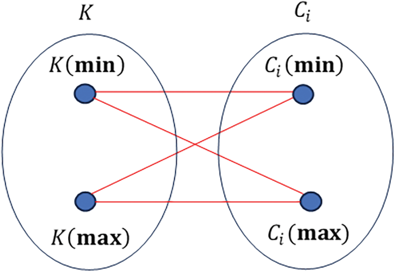
Figure 1: Relations between an artificial class space and i-th class space

No crossing edges are allowed in the graph. It implies the existence of only one-to-one relationships between K and Ci spaces. In order to meet this condition, the original graph is partitioned into two subgraphs, G(min) and G(max), as depicted in Fig. 2.

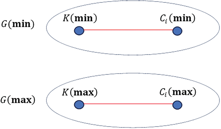
Figure 2: Disjoint subgraphs of an original graph

Let K(min) and Ci(min) be a minimum class subspace of an artificial class and minimum subspace of the i-th class space, respectively, then the absolute p–difference between these subspaces equals:

Λi,p(min,min):=|Kp(min)−Cip(min)|1p,∀i∈[1,m](27)

Analogically, this study defines absolute p–difference for max subspaces:

Λi,p(max,max):=|Kp(max)−Cip(max)|1p,∀i∈[1,m](28)

For rock mass quality assessment, the value of p is p≥2. This study adopts p=2. The intensity of the integrated absolute p–difference is defined as follows:

Λi,2=Λi,22(min,min)+Λi,22(max,max)=|K2(min)−Ci2(min)|+|K2(max)−Ci2(max)|,∀i∈[1,m](29)

Finally, the discriminant function (classifier) is defined as follows:

C=max{Λi,2}=max{|K2(min)−Ci2(min)|+|K2(max)−Ci2(max)|},i=1,2,…,m(30)

A class with the highest value of {Λi,2},i=1,2,…,m is a class of a sample Y.

The methodology for determining the rock mass class of surrounding rock is shown in the following graphical way (Fig. 3).

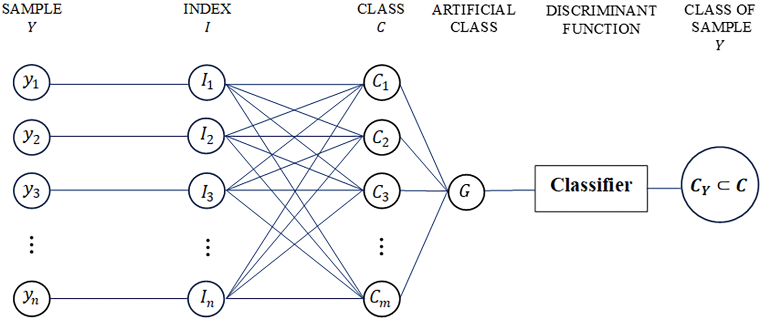
Figure 3: Graphical presentation of the rock mass quality assessment

The developed algorithm for the same purpose is depicted in Fig. 4.

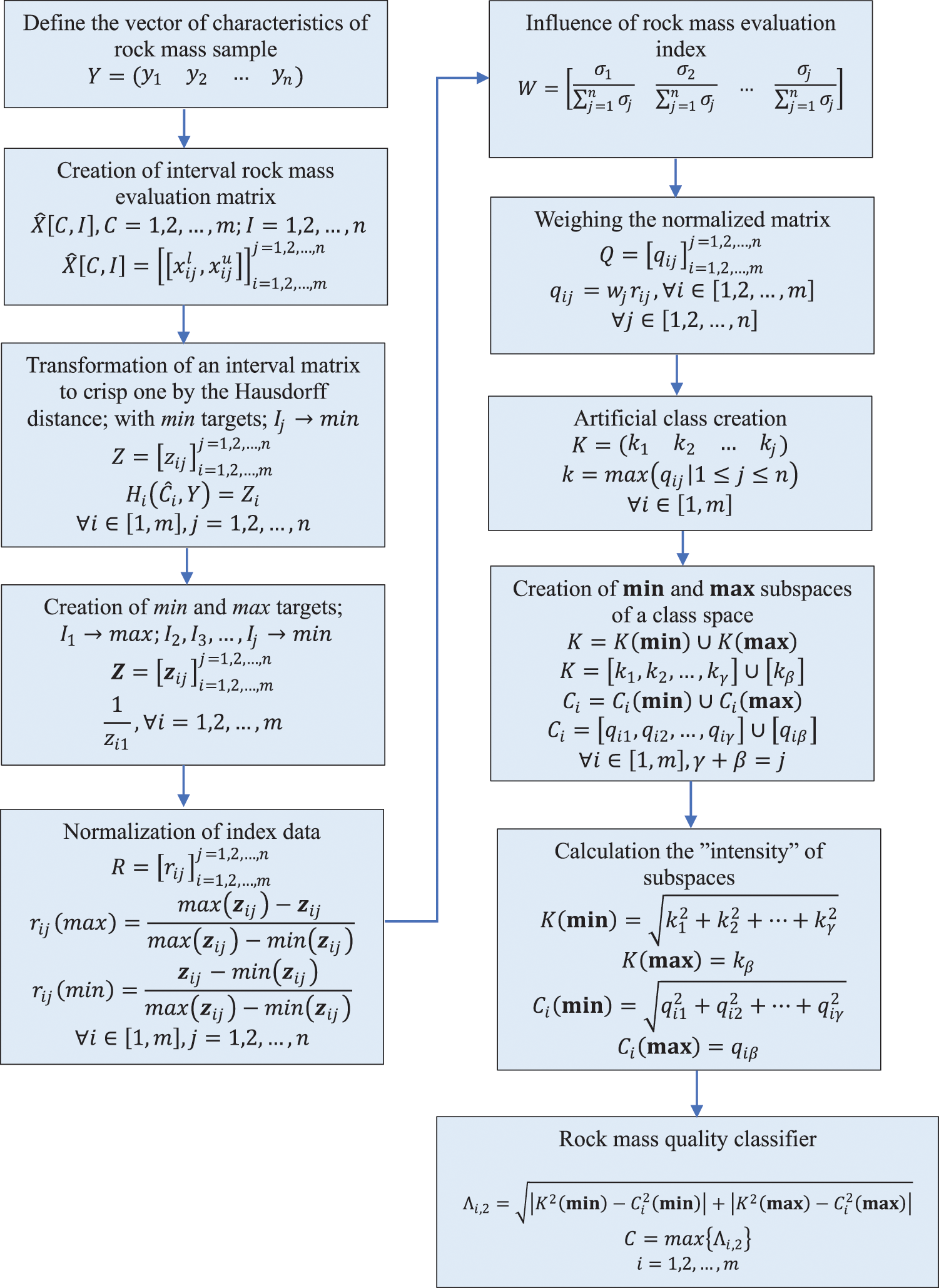
Figure 4: Flowchart for the rock mass quality assessment based on the Gromov-Hausdorff distance

3  Numerical Example

This section uses three numerical examples from different studies to validate the developed method. Classes obtained by the GHDQR method are compared to classes obtained by other methods.

3.1 Example One

The underground engineering of the Guangzhou Pumped Storage Power Station is considered an engineering example to evaluate the efficiency of the developed methodology. The stability of the surrounding rock is affected by many parameters. In this comparison, the research applies the following parameters, i.e., rock mass evaluation indices [8]:

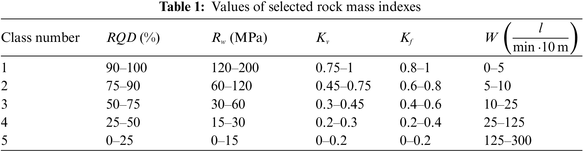
a)   the rock quality index RQD (%),

b)   uniaxial saturated compressive strength Rw (MPa),

c)   integrity coefficient Kv,

d)   structural plane strength coefficient Kf,

e)   groundwater seepage quantity W(lmin⋅10m).

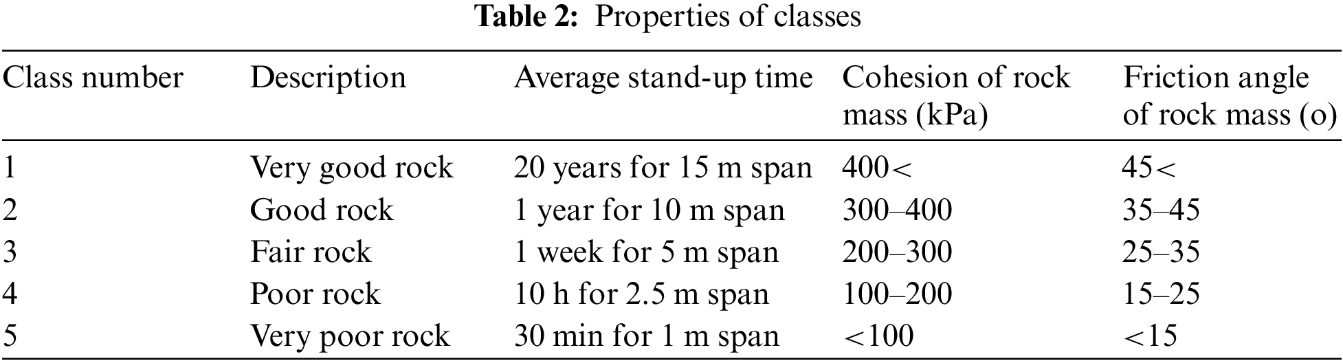
The stability of surrounding rock is divided into the following five classes based on the previously selected rock mass evaluation indices (Table 1) [8].

The properties of each class are presented in Table 2 [38].

Interval matrix X^, which presents the relationship between five classes and a set of five rock mass evaluation indices, is described as follows:

X^=[[xijl,xiju]]i=1,2,…,5j=1,2,…,5=[C,II1I2I3I4I5targetmaxmaxmaxmaxminC1[90,100][120,200][0.75,1][0.8,1][0,5]C2[75,90][60,120][0.45,0.75][0.6,0.8][5,10]C3[50,75][30,60][0.3,0.45][0.4,0.6][10,25]C4[25,50][15,30][0.2,0.3][0.2,0.4][25,125]C5[0,25][0,30][0,0.2][0,0.2][125,300]](31)

Sample vector, with values of RQD, Rw, Kv, Kf, and W is:

Y=(71.890.10.570.450)(32)

For the RQD index, the Hausdorff distance between matrix element [x11l,x11u] and vector element y1 equals:

H([90,100],[71.8,71.8])=max{|90−71.8|,|100−71.8|}=28.2(33)

Analogically, the following matrix Z of the Hausdorff distances is obtained:

Z=[zij]i=1,2,…,5j=1,2,…,5=[C,II1I2I3I4I5targetminminminminminC128.20109.900.430.555.00C218.2030.100.180.3510.00C321.8060.100.270.1525.00C446.8075.100.370.25125.00C571.7990.090.560.44300.00](34)

Since all indexes I1, I2, I3, I4, and I5 tend to achieve min value as the best one, it is necessary to create min and max targets. This study selects the index I1 to be transformed into max target. The reciprocal value of the element z11 is as follows:

z11=128.20=0.03546(35)

Values of the elements z12, z13, z14, and z15 are calculated analogically, and the new transformed matrix Z is as follows:

Z=[zij]i=1,2,…,5j=1,2,…,5=[C,II1I2I3I4I5targetmaxminminminminC10.03546109.900.430.555.00C20.0549530.100.180.3510.00C30.0458760.100.270.1525.00C40.0213775.100.370.25125.00C50.0139390.090.560.44300.00](36)

Values of the remaining indices for classes hold the same values as in the matrix Z. This research continues with creating a dimensionless matrix R by the normalization process. For max target value of the RQD index, the normalization of the element z11 is as follows:

r11(max)=0.05495−0.035460.05495−0.01393=0.47504(37)

For min target value of the RQD index, the normalization of the element z15 is:

r15(min)=5−5300−5=0(38)

Accordingly, the normalized matrix R is produced with the following values of its elements:

R=[rij]i=1,2,…,5j=1,2,…,5=[C,II1I2I3I4I5targetmaxminminminminC10.475041.000000.657891.000000.00000C20.000000.000000.000000.500000.01695C30.221220.375940.236840.000000.06780C40.818650.563910.500000.250000.40678C51.000000.751751.000000.725001.00000](39)

The influence (weight) of each index is calculated using the standard deviation method. The vector of the standard deviation is as follows:

σ=[0.412260.379310.384700.391470.42586](40)

Weights w1 of index I1 equals:

w1=0.412260.41226+0.37931+0.38470+0.39147+0.42586(41)

Analogically, the weights of indices I2, I3, I4, I5, and their values are calculated as follows:

W=[0.206790.190270.192970.196360.21361](42)

Weighted normalized element q11 is calculated as the product of the weight of the index I1 and normalized value of the RQD for class 1:

q11=0.20679⋅0.47504=0.09823(43)

In the same way, the rest of the weighted normalized elements are calculated, and the outcome of the calculation is presented by matrix Q:

Q=[qij]i=1,2,…,5j=1,2,…,5=[C,II1I2I3I4I5targetmaxminminminminC10.098230.190270.126950.196360.00000C20.000000.000000.000000.098180.00362C30.045750.071530.045700.000000.01448C40.169290.107290.096480.049090.08689C50.206790.143030.192970.142360.21361](44)

The artificial value of index I1 is extracted using Eq. (17) as follows:

k1=max(0.098230.000000.045750.169290.20679)=0.2067(45)

The artificial class space is yielded by applying the same equation to the rest of the indices as follows:

K=(0.206790.190270.192970.196360.21361)(46)

It is necessary to define elements of these subspaces while respecting the prerequisite of existing min and max subspaces of each class space. Artificial class space K presents the union of the subspace K(min) and subspace K(max):

K=K(min)∪K(max)=[k2,k3,k4,k5]∪[k1](47)

K=K(min)∪K(max)=[0.19027,0.19297,0.19636,0.21361]∪[0.20679](48)

Class space C1 presents the union of the subspace C1(min) and subspace C1(max):

C1=C1(min)∪C1(max)=[q12,q13,q14,q15]∪[q11](49)

C1=[0.19027,0.12695,0.19636,0.00000]∪[0.09823](50)

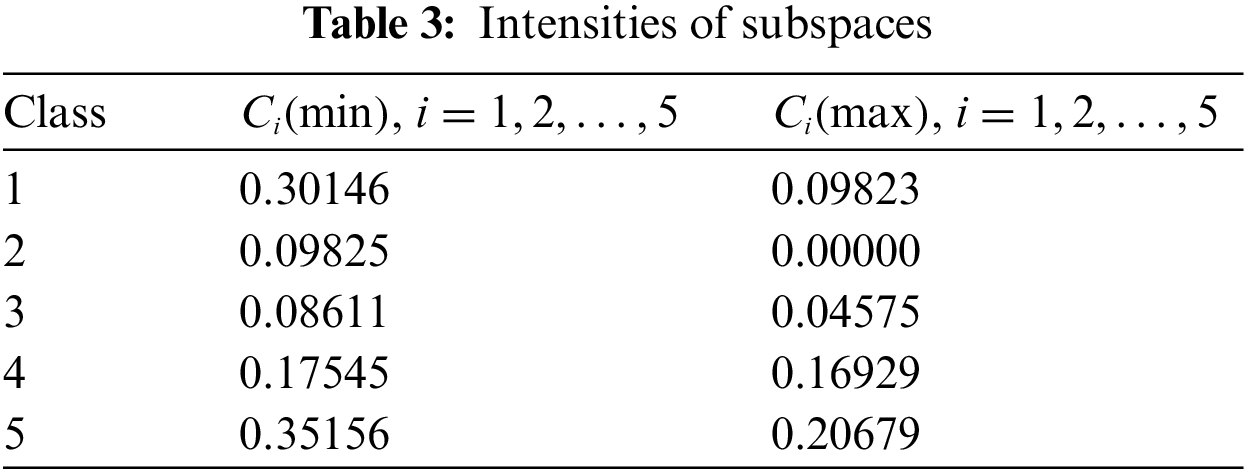
Following the calculation of the intensity of subspaces K(min) and K(max), the results are presented as follows:

K(min)=0.190272+0.126952+0.196362+0.213612=0.39702(51)

K(max)=0.20679(52)

Intensities of C1(min) and C1(max) are as follows:

C1(min)=0.190272+0.126952+0.196362+0.000002=0.30146(53)

C1(max)=0.09823(54)

The same way is applied to get subspaces of classes C2,C3,C4,C5, and their intensities. Table 3 shows the intensities of subspaces.

The absolute p–difference between subspaces K(min) and C1(min) for class 1, equals:

Λ1,2(min,min):=|K2(min)−C12(min)|12=|0.397022−0.301462|12=0.25836(55)

The absolute p–difference between subspaces G(max), C1(max), for class 1, equals:

Λ1,2(max,max):=|K2(max)−C12(max)|12=|0.206792−0.098232|12=0.18197(56)

The intensity of the integrated absolute p–difference for class 1 is as follows:

Λ1,2=0.258362+0.181972=0.31601(57)

Intensities of the absolute p–differences for all classes are listed in Table 4.

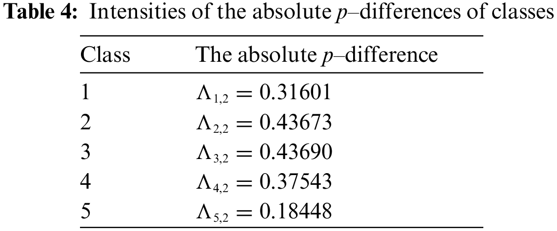
The value of the discriminant function (classifier) of the rock sample is determined using Eq. (30) as follows:

C=max{0.31601,0.43673,0.43690,0.37543,0.18448}=0.43690(58)

Since Λ3,2=0.43690 is the maximum value, which indicates that the rock sample belongs to Class 3, with properties defined in Table 2.

A developed rock mass classifier was applied to thirty rock samples, and the classification results are presented in Table 5 and Fig. 5.

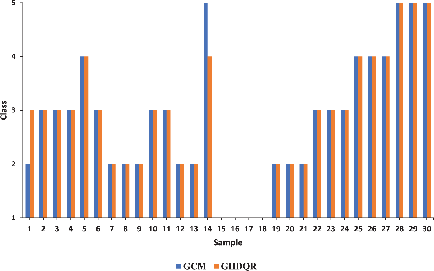
Figure 5: Comparison results between the obtained and actual values

In two cases, the GHDQR model missed actual values. It happened in Samples 1 and 14. The model assigned one class lower on Sample 1 and one class higher on Sample 4. MAPE was employed to analyze the efficiency of the GHDQR method. The following equation defines it:

MAPE=∑i=1N|Ca−CGHDQRCa|×100\% (59)

where:

Ca is the actual class of rock mass

CGHDQR is class obtained by developed methodology

N is the total number of rock samples

In this comparison, MAPE equals:

MAPE=0.730×100\% =2.33%(60)

3.2 Example Two

This subsection will not present detailed calculus, as in the previous one, but only the obtained results and comparison indicators. This comparison is conducted using data obtained from the literature [27]. Classification indices for rock mass quality grades are previously listed in Table 1. A developed rock mass classifier is applied to seventeen rock samples, and the classification results are depicted in Table 6 and Fig. 6. The literature [27] used the following four methods for classification: Discriminant, Mutation series, ANN, and SVM.

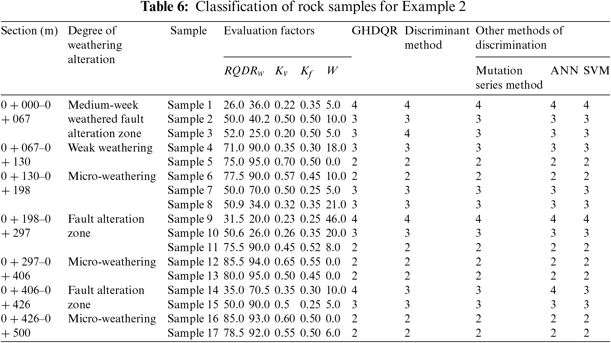
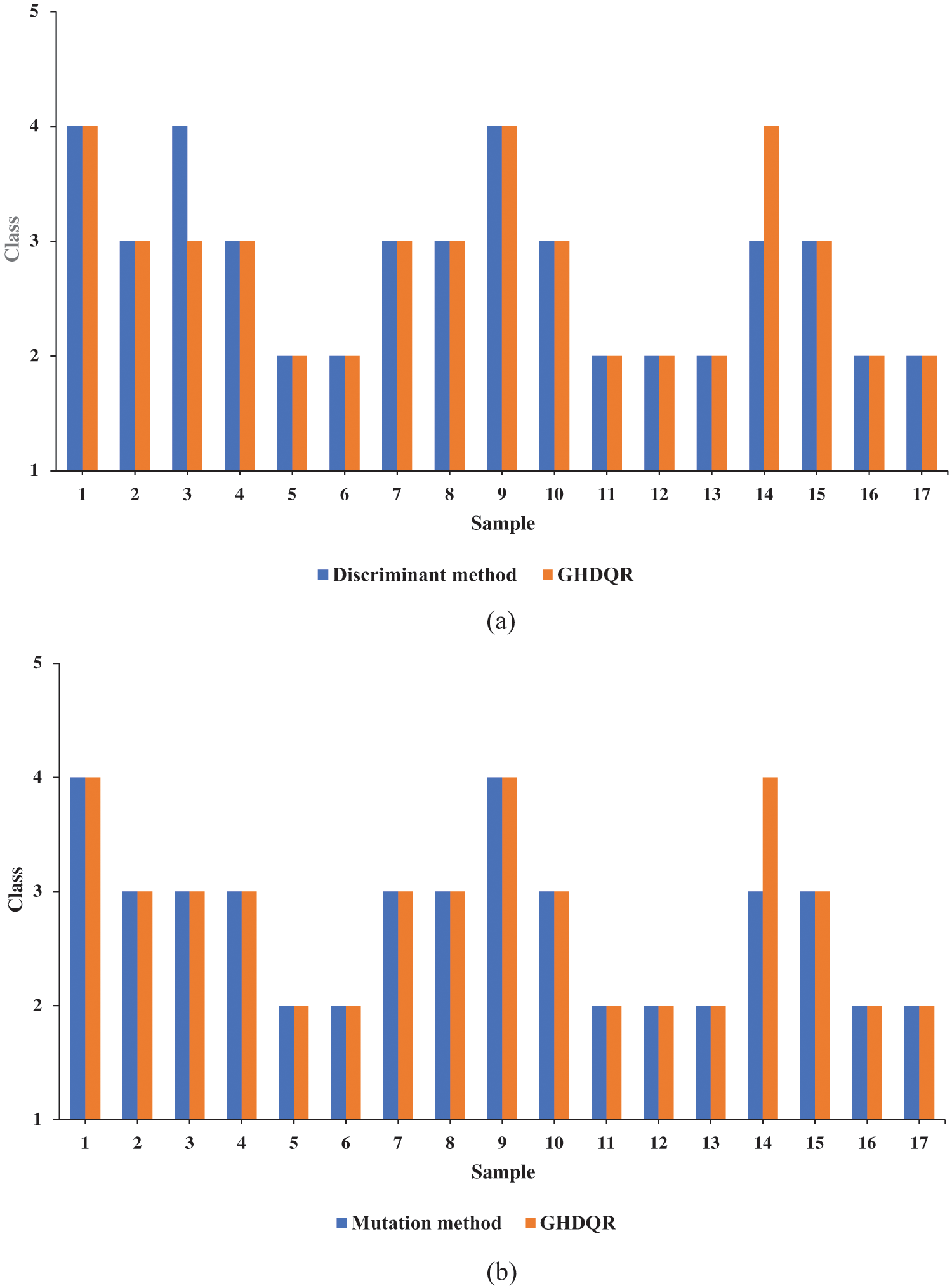
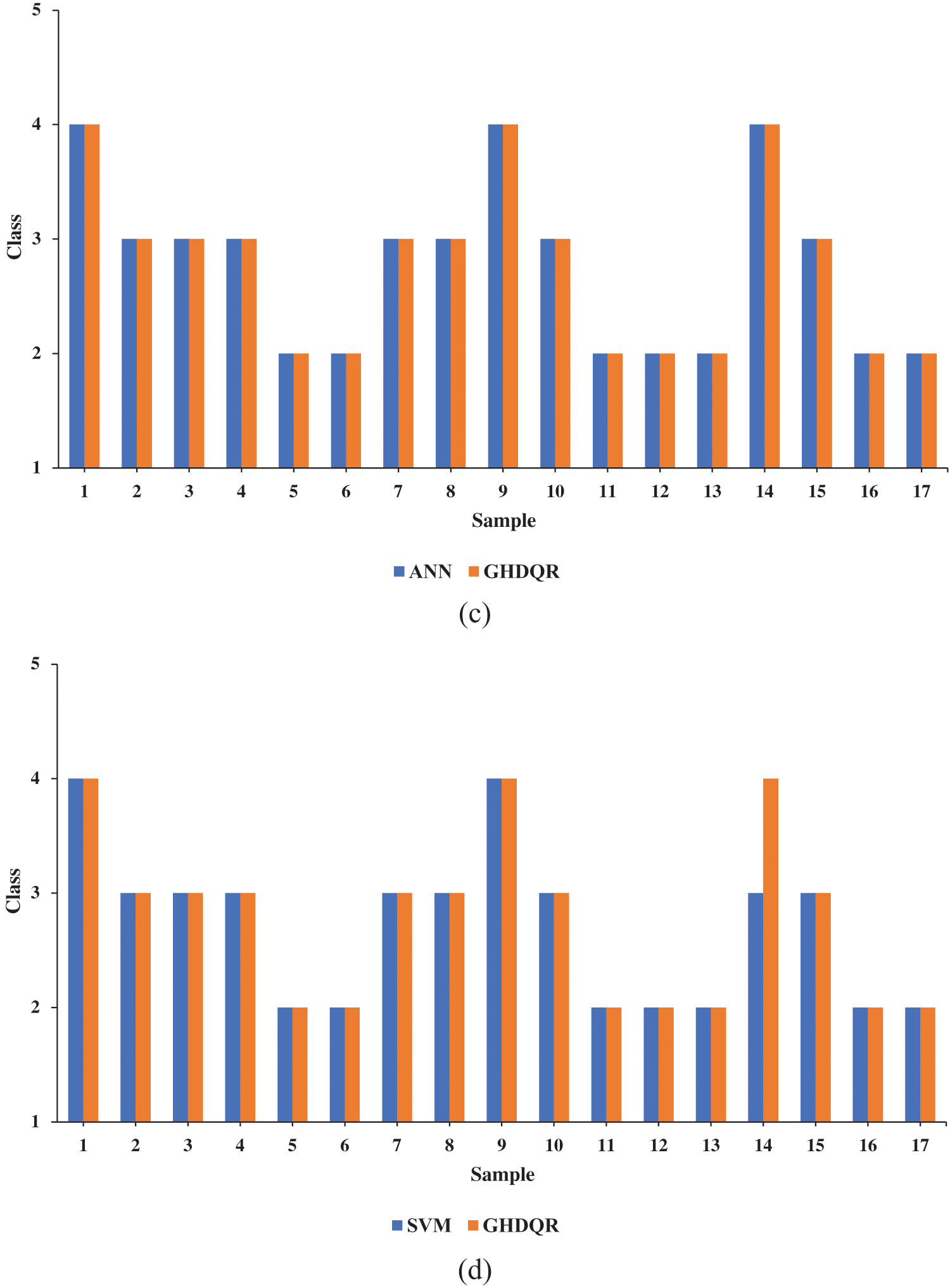
Figure 6: Comparison results between the obtained and actual values: (a) Discrimination method, (b) Mutation method, (c) ANN, (d) SVM

The efficiency of the GHDQR method for the Discrimination, Mutation, ANN, and SVM is listed in Table 7.

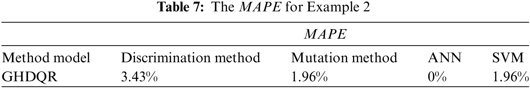
GHDRQ-Discrimination method: in two cases, the GHDQR model missed actual values. It occurred in Samples 3 and 14. The model assigned one class higher on Sample 3 and one lower on Sample 14. The MAPE is 3.43%.

GHDRQ-Mutation method: in one case, the GHDQR model missed actual values. It occurred on Sample 14. The model assigned one class lower than the actual one. The MAPE is 1.96%.

GHDRQ-ANN method: there are no missed values. The MAPE is 0%.

GHDRQ-ANN method: The same result was obtained as the GHDQR-Mutation method.

The average value of the MAPE for these four comparisons is 1.84%.

Fig. 6 and Table 7 indicate that the GHDQR methodology is compared to four rock mass classification methods: Discrimination, Mutation, ANN, and SVM. The results clearly show that the relationship between the methods compared to the proposed method is very high. It is also proven by the average value of the MAPE with 1.84%. It indicates highly accurate compatibility between results obtained by the proposed method and results obtained by the abovementioned methods. The developed method aligns with the compared methods and can be applied to classify different rock samples.

3.3 Example Three

This comparison adopted data from the literature [17]. The selected rock mass indices are:

f)   Uniaxial saturated compressive strength Rw (MPa),

g)   Rock quality index RQD (%),

h)   Integrity coefficient Kv,

i)   Groundwater seepage quantity W (lmin⋅10m).

Table 1 shows the indices values. The developed GHDQR classifier was applied to nine rock samples, and the classification results are listed in Table 8 and Fig. 7.

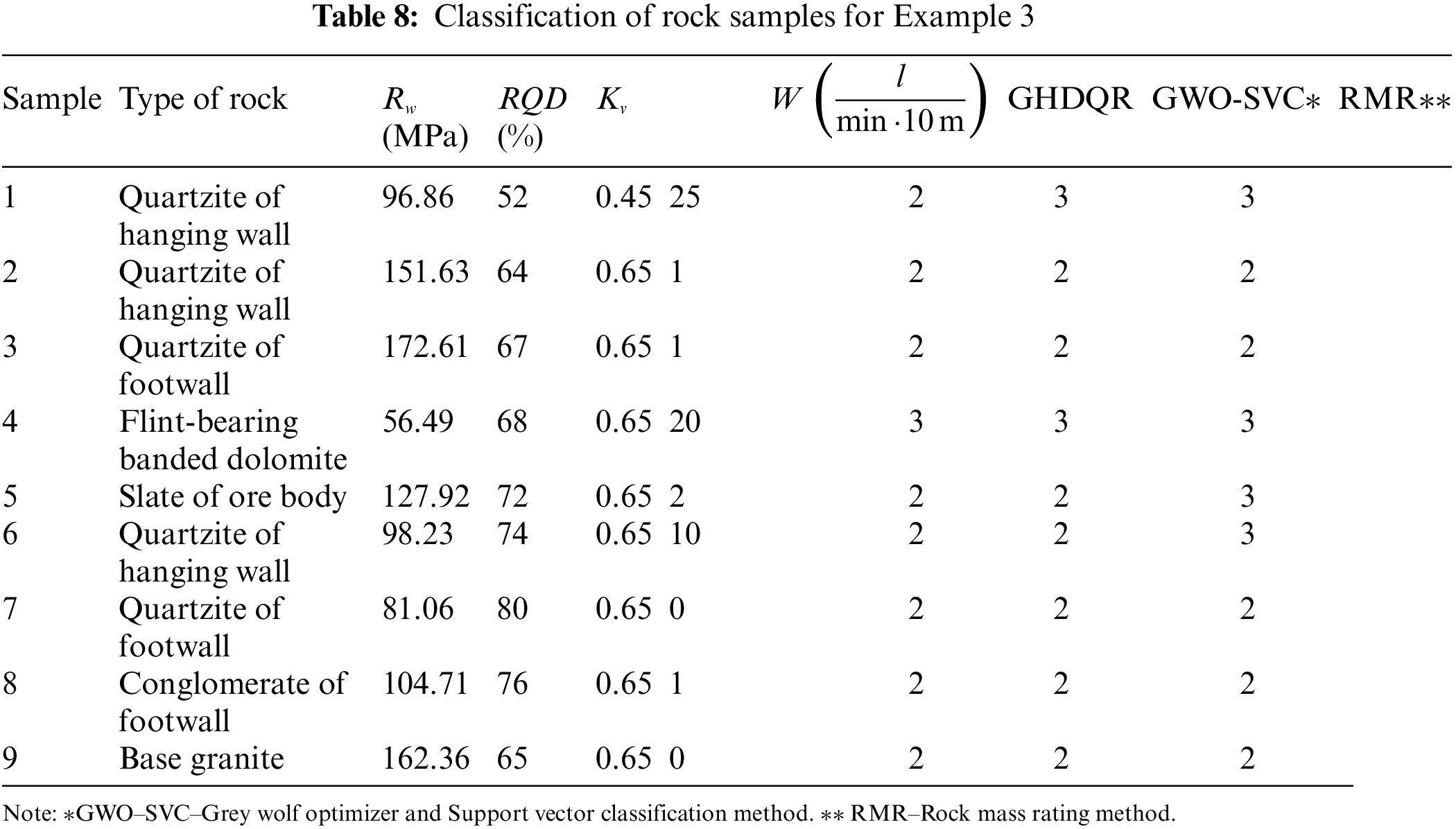
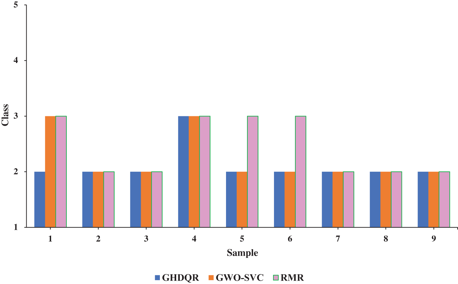
Figure 7: Comparison results between the GHDQR, GWO-SVC and RMR methods

The MAPE between methods, which have been mutually compared, is presented in Table 9.

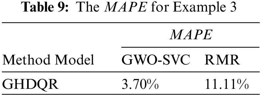
The average value of the MAPE for the GHDQR method is 7.41%.

3.4 Sensitivity Analysis

The following part presents the sensitivity analysis of the proposed methodology. As part of the sensitivity analysis, the variation of the parameter p within the expression (26) is analyzed. The initial results shown in the examples are defined for the values of the parameter p=2. Since the parameter p can have values from the interval p∈[1,∞)in the following section, the influence of other values p∈[1,∞) on the model results is analyzed.

Since the value of the parameter p is defined based on subjective assessments, in the following part, the dependence of the results on the value of the specified parameter (for example one) is considered. To examine the influence of the parameter p, thirty scenarios are generated. In the first scenario, the value of p=2 is adopted, while in each subsequent scenario, the value of p is increased by one. Fig. 8 depicts the values of Λp generated for parameter values 2≤p≤30.

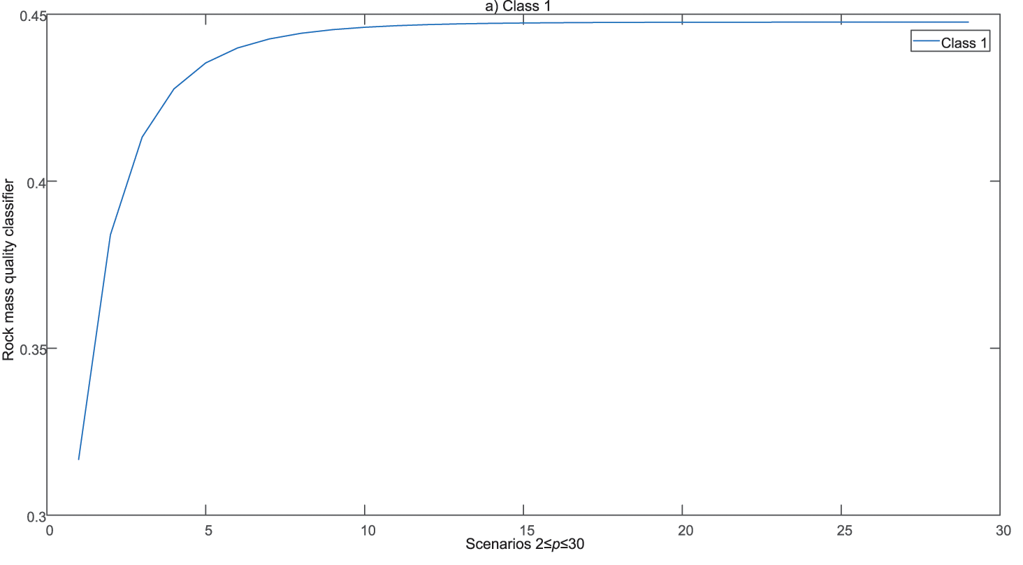
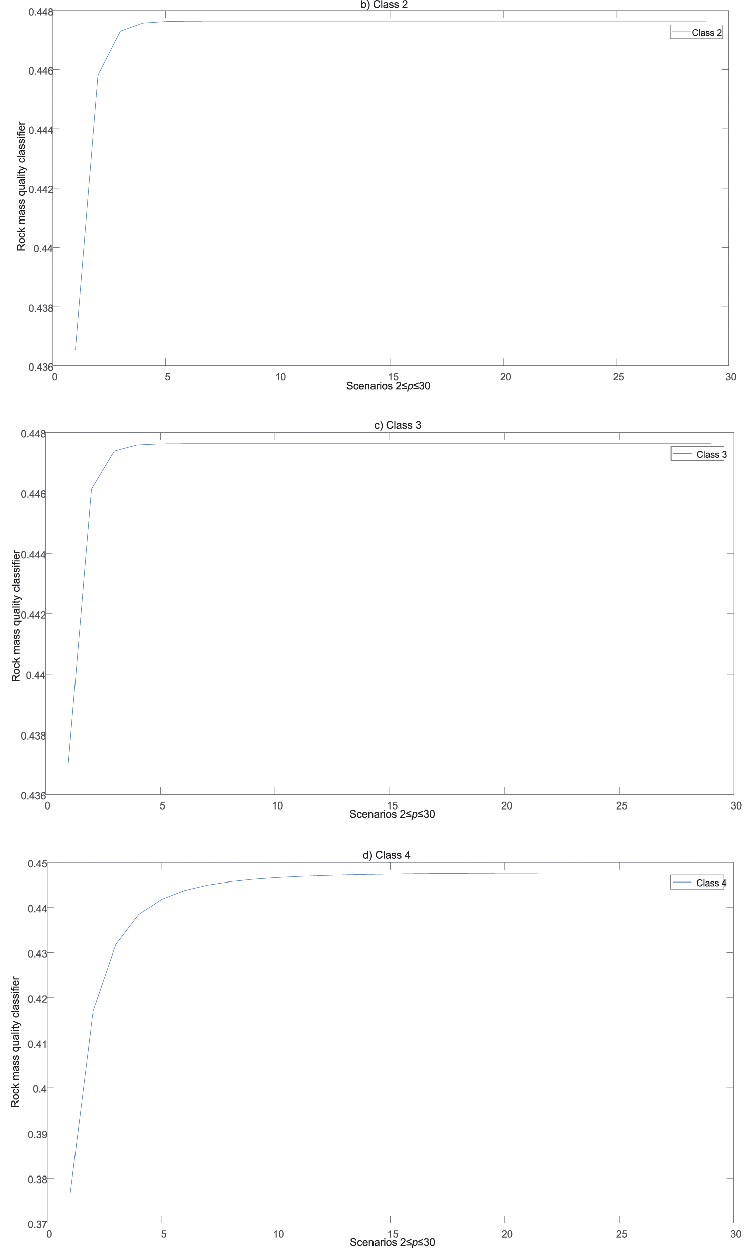
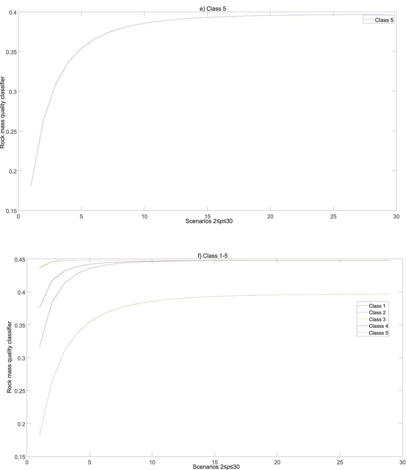
Figure 8: Rock mass quality classifier values for 2≤p≤30: (a) class 1, (b) class 2, (c) class 3, (d) class 4, (e) class 5, (f) summarized class 1–5

Fig. 8a through 8f indicate that the parameter p affects the variation of Λp, and thus the results. By analyzing the presented results, increasing the parameter p impacts the approximation of the value Λp. The choice of the value of the parameter p>5 makes it difficult to choose the dominant Class clearly; hence, it is recommended to adopt a value in the interval 2≤p≤5 to define the initial solution. Fig. 8f shows that Class 3 represents the dominant solution in example one.

The graphical interpretation of the results of the change of the parameter 2≤p≤30 is depicted in Fig. 8. The variations in the parameter p caused a change in the value of the rock mass quality classifier and selection of the dominant Class. For easier monitoring of changes in the dominant Class during the simulation, the results are listed in Table 10. Table 10 presents the rock mass quality in example one during the considered thirty scenarios (2≤p≤30).

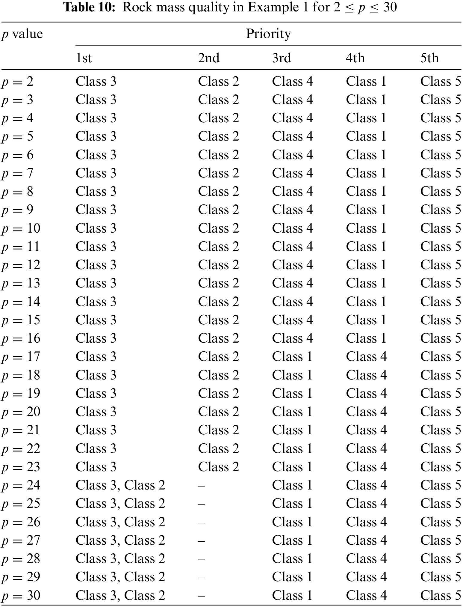
Table 10 shows that for all values of the parameter p, Class 3 illustrates the dominant solution from the considered set. Since the statistical correlation of the results across the scenarios is high, it can be concluded that the initial solution was confirmed. A similar analysis was performed for examples two and three, which is omitted in this paper.

3.5 Summary Discussion on Comparison and Model

In Section 3, the Gromov-Hausdorff distance for quality of rock method was compared to the following seven methods:

1.   Gaussian cloud method,

2.   Discriminant method,

3.   Mutation series method,

4.   ANN,

5.   SVM,

6.   GWO-SVC,

7.   RMR.

Comparisons were conducted for the following five-rock mass evaluation indices:

j)   Rock quality index RQD (%),

k)   Uniaxial saturated compressive strength Rw (MPa),

l)   Integrity coefficient Kv,

m)   Structural plane strength coefficient Kf,

n)   Groundwater seepage quantity W (lmin⋅10m)

Table 11 details the interpretation of typical MAPE values [39].

The MAPE scale in Table 11 can be treated as a rigorous approach, as there are only four categories. Each category is defined by adequate numerical value and associated linguistic description. Based on the obtained numerical values of comparisons, the MAPE of the GHDQR method is illustrated in Table 12.

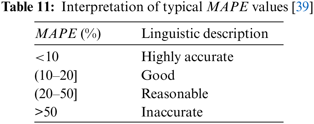
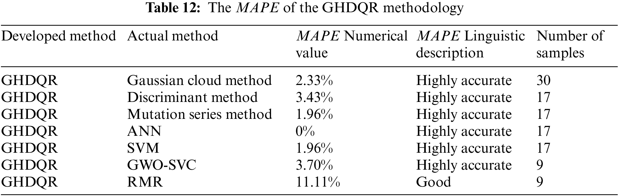
The comparisons demonstrated that the classification results of the model are consistent with the actual classes obtained by the mentioned methods. The share of the highly accurate category is 85.71%, while the share of the good category is 14.29%. It indicates that the GHDQR methodology is feasible for surrounding rock quality classification.

Compared to other rock mass classification methods, the GHDQR method is a transparent tool for asses the quality of the rock sample. GHDQR methodology consists of a total of twelve steps. Each step is described in detail by the mathematical formulas and graphically illustrated through the flowchart of the model. Also, the exhaustive step-by-step presentation of numerical examples shows a high level of explainability and interpretability. The proposed methodology is simple and easy to understand. Although this methodology consists of twelve steps, it does not require high computational time. The algorithm is not limited to the input data size, which indicates the developed model’s great stability and reliability. Considering all these positive aspects, the proposed GHDQR methodology presents a powerful tool for analyzing the rock mass and rock sample classification.

The performances of the GHDQR method are listed as follows: data type is quantitative, MAPE is highly accurate, transparency is good, the complexity of the method is less, consumption time is low, and mathematical calculus required is low. The GHDQR method for assessing rock mass quality is a reliable tool that is easy to understand and implement.

4  Conclusion

This study develops an innovative approach for rock mass quality rating in a multi-criteria grey environment named GHDQR. It proposes a new discriminant function (classifier) based on the Gromov-Hausdorff metric space distance for assessing rock mass quality. These metric spaces are the rock mass evaluation matrix and rock sample vector. The algorithm can deal with uncertainties of input data, as interval-grey numbers express the elements of the matrix. The performance of the proposed methodology is verified by comprehensive comparative analysis through the three numerical examples, showing its strength and stability. Several advantages can be observed from the obtained results:

o)   A developed classifier objectively defines the class of rock samples, with no experts interfering in the classification process.

p)   The GHDQR method is simple and easy to understand, minimal mathematical calculation is required, and transparency is good.

q)   Compared to seven actual methods, the developed model produces high-accuracy results and aligns with all mentioned methods.

r)   The GHDQR can be a valuable and reliable rock mass classification tool from all these positive aspects.

The study has several limitations that can be analyzed in the future. One of the limitations of the proposed methodology can be reflected in the fact that a case study with actual data is not presented but only through a comparative analysis. Mining engineers must understand this developed model and compare the results obtained with our original values. Another limitation can be observed in the number of parameters evaluating the rock mass. Only five-rock mass evaluation indices are considered in the proposed model, which should be improved for more parameters such as discontinuity and groundwater conditions.

Future research will focus on developing a model capable of processing more rock samples and hydraulic radius simultaneously to assess the conditions for bulk underground mining methods, such as block caving, sublevel caving, and longwall mining. Another direction of future research will include actual data, i.e., a case study where the results will verify the proposed methodology’s practical implication and efficiency. Also, the specific numerical example should be extended to include the number of parameters evaluating the rock mass in future research. From the point of view of mathematical calculation, future research can include other techniques for calculating the distance metrics such as Euclidean distance, Chebyshev distance, Manhattan distance, and others. By performing a detailed comparative analysis of these methods, the most suitable distance methodology can be selected as the best one. Also, by combining these approaches, hybrid methods for rock mass classification can be created.

Acknowledgement: The authors would like to thank the unknown reviewers for their valuable suggestions and greatly appreciate the time spent in reviewing.

Funding Statement: The authors received no specific funding for this study.

Author Contributions: The authors confirm their contribution to the paper as follows: study conception and design: MG, ZG; data collection: SJ, SL; analysis and interpretation of results: DP, IJ; draft manuscript preparation: MG, ZG. All authors reviewed the results and approved the final version of the manuscript.

Availability of Data and Materials: The data utilized in this study is fully documented within the paper. Should there be any inquiries, please feel free to contact the authors.

Conflicts of Interest: The authors declare that they have no conflicts of interest to report regarding the present study.

References

1. Wu S, Du X, Yang S. Rock mass quality evaluation based on unascertained measure and intuitionistic fuzzy sets. Complexity. 2020;2020:1–14. doi:10.1155/2020/5614581. [Google Scholar] [CrossRef]

2. Mao X, Hu A, Zhao R, Wang F, Wu M. Evaluation and application of surrounding rock stability based on an improved fuzzy comprehensive evaluation method. Mathematics. 2023;11:3095. doi:10.3390/math11143095. [Google Scholar] [CrossRef]

3. Nikafshan Rad H, Jalali Z. Modification of rock mass rating system using soft computing techniques. Eng Comput. 2019;35(4):1333–57. doi:10.1007/s00366-018-0667-6. [Google Scholar] [CrossRef]

4. Shao JL, Gao L, Wu QH, Gu XB. The application of variable fuzzy sets theory on the quality assessment of surrounding rocks. Adv Mater Sci Eng. 2022;2022:5441829. doi:10.1155/2022/5441829. [Google Scholar] [CrossRef]

5. Ataei M, Besheli AD, Sereshki F, Jamshidi M. An application of fuzzy sets to the rock mass rating (RMR) system used in rock engineering; a case study in Iran. In: Proceedings of the 8th International Scientific Conference-SGEM2008; 2008 Jun 16–20; Albena, Bulgaria. p. 347–56. [Google Scholar]

6. Namin FS, Rinne M, Rafie M. Uncertainty determination in rock mass classification when using FRMR Software. J S Afr Inst Min Metall. 2015;115(11):1073–82. doi:10.17159/2411-9717/2015/v115n11a12. [Google Scholar] [CrossRef]

7. Zhang J, Shi K, Majiti H, Shan H, Fu T, Shi R, et al. Study on the classification and identification methods of surrounding rock excavatability based on the rock-breaking performance of tunnel boring machines. Appl Sci. 2023;13:7060. doi:10.3390/app13127060. [Google Scholar] [CrossRef]

8. Teng Y, Zhou K, Li Z. Classification of underground engineering surrounding rock based on Gaussian cloud model. J Phys Conf Seri. 2021;1983(1):012024. doi:10.1088/1742-6596/1983/1/012024. [Google Scholar] [CrossRef]

9. Mohammadi M, Hossaini MF. Modification of rock mass rating system: interbedding of strong and weak rock layers. J Rock Mech Geotech Eng. 2017;9(6):1165–70. doi:10.1016/j.jrmge.2017.06.002. [Google Scholar] [CrossRef]

10. Sebbeh-Newton S, Ismail S, Zabidi H. Prediction of rock mass rating using adaptive neuro-fuzzy inference system (ANFIS) for NATM-3 of Pahang-Selangor raw water transfer tunnel (PSRWT) project, Malaysia. AIP Conf Proc. 2020;2267(1):020021. doi:10.1063/5.0016415. [Google Scholar] [CrossRef]

11. Jalalifar H, Mojedifar S, Sahebi A. Prediction of rock mass rating using fuzzy logic and multi-variable RMR regression model. Int J Min Sci Technol. 2014;24:237–44. doi:10.1016/j.ijmst.2014.01.015. [Google Scholar] [CrossRef]

12. Liu YC, Chen CS. A new approach for application of rock mass classification on rock slope stability assessment. Eng Geol. 2007;89:129–43. doi:10.1016/j.enggeo.2006.09.017. [Google Scholar] [CrossRef]

13. Wu LZ, Li SH, Zhang M, Zhang LM. A new method for classifying rock mass quality based on MCS and TOPSIS. Environ Earth Sci. 2019;78:199. doi:10.1007/s12665-019-8171-x. [Google Scholar] [CrossRef]

14. Song S, Xu Q, Chen J, Zhang W, Cao C, Li Y. Engineering classification of jointed rock mass based on connectional expectation: a case study for Songta dam site, China. Adv Civ Eng. 2020;2020:1–15: 3581963. doi:10.1155/2020/3581963. [Google Scholar] [CrossRef]

15. Gu XB, Ma Y, Wu QH, Liu YB. The application of intuitionistic fuzzy set-TOPSIS model on the level assessment of the surrounding rocks. Shock Vib. 2022;2022:4263276. doi:10.1155/2022/4263276. [Google Scholar] [CrossRef]

16. Zheng S, Jiang A, Yang X, Luo G, Pham BT. A new reliability rock mass classification method based on least squares support vector machine optimized by bacterial foraging optimization algorithm. Adv Civ Eng. 2020;2020:3897215. doi:10.1155/2020/3897215. [Google Scholar] [CrossRef]

17. Hu J, Zhou T, Ma S, Yang D, Guo M, Huang P. Rock mass classification prediction model using heuristic algorithms and support vector machines: a case study of Chambishi copper mine. Sci Rep. 2022;12(1):928. doi:10.1038/s41598-022-05027-y. [Google Scholar] [PubMed] [CrossRef]

18. Sheng D, Yu J, Tan F, Tong D, Yan T, Lv J. Rock mass quality classification based on deep learning: a feasibility study for stacked autoencoders. J Rock Mech Geotech Eng. 2023;15(7):1749–58. doi:10.1016/j.jrmge.2022.08.006. [Google Scholar] [CrossRef]

19. Azarafza M, Hajialilue Bonab M, Derakhshani R. A deep learning method for the prediction of the index mechanical properties and strength parameters of marlstone. Materials. 2022;15:6899. doi:10.3390/ma15196899. [Google Scholar] [PubMed] [CrossRef]

20. Santos AEM, Lana MS, Pereira TM. Evaluation of machine learning methods for rock mass classification. Neural Comput Appl. 2022;34:4633–42. doi:10.1007/s00521-021-06618-y. [Google Scholar] [CrossRef]

21. Cheng X, Tang H, Wu Z, Liang D, Xie Y. BILSTM-based deep neural network for rock-mass classification prediction using depth-sequence MWD data: a case study of a tunnel in Yunnan, China. Appl Sci. 2023;13:6050. doi:10.3390/app13106050. [Google Scholar] [CrossRef]

22. Gholami R, Rasouli V, Alimoradi A. Improved RMR rock mass classification using artificial intelligence algorithms. Rock Mech Rock Eng. 2013;46:1199–209. doi:10.1007/s00603-012-0338-7. [Google Scholar] [CrossRef]

23. Hou S, Liu Y, Yang Q. Real-time prediction of rock mass classification based on TBM operation big data and stacking technique of ensemble learning. J Rock Mech Geotech Eng. 2021;14:123–43. doi:10.1016/j.jrmge.2021.05.004. [Google Scholar] [CrossRef]

24. Yang G, Li TB, Ma CC, Meng LB, Zhang HG, Ma JJ. Intelligent rating method of tunnel surrounding rock based on one-dimensional convolutional neural network. J Intell Fuzzy Syst. 2022;42(3):2451–69. doi:10.3233/JIFS-211718. [Google Scholar] [CrossRef]

25. Yalcin I, Can R, Kocaman S, Gokceoglu C. Rock mass discontinuity determination with transfer learning. Int Arch Photogramm Remote Sens Spatial Inf Sci. 2023;48:609–14. doi:10.5194/isprs-archives-XLVIII-M-1-2023-609-2023. [Google Scholar] [CrossRef]

26. Alzubaidi F, Mostaghimi P, Si G, Swietojanski P, Armstrong RT. Automated rock quality designation using convolutional neural networks. Rock Mech Rock Eng. 2022;55(6):3719–34. doi:10.1007/s00603-022-02805-y. [Google Scholar] [CrossRef]

27. Wang J, Guo J. Research on rock mass quality classification based on an improved rough set-cloud model. IEEE Access. 2019;7:123710–24. doi:10.1109/ACCESS.2019.2938567. [Google Scholar] [CrossRef]

28. Tan F, You M, Zuo C, Jiao YY, Tian H. Simulation of rock-breaking process by drilling machine and dynamic classification of surrounding rocks. Rock Mech Rock Eng. 2022;55(1):423–37. doi:10.1007/s00603-021-02659-w. [Google Scholar] [CrossRef]

29. Riazi E, Yazdani M, Afrazi M. Numerical study of slip distribution at pre-existing crack in rock mass using extended finite element method (XFEM). Iran J Sci Technol Trans Civil Eng. 2023;47(4):2349–63. [Google Scholar]

30. Majedi MR, Afrazi M, Fakhimi A. A micromechanical model for simulation of rock failure under high strain rate loading. Int J Civ Eng. 2021;19(5):501–15. [Google Scholar]

31. Zhang Y, Zhuang X. Cracking elements: a self-propagating strong discontinuity embedded approach for quasi-brittle fracture. Finite Elem Anal Des. 2018;144:84–100. [Google Scholar]

32. Zhang Y, Mang HA. Global cracking elements: a novel tool for Galerkin-based approaches simulating quasi-brittle fracture. Int J Numer Methods Eng. 2020;121(11):2462–80. [Google Scholar]

33. Liu S, Fang Z, Yang Y, Forrest J. General Grey numbers and their operations. Grey Syst Theory Appl. 2012;2(3):341–9. doi:10.1108/20439371211273230. [Google Scholar] [CrossRef]

34. Szmidt E, Kacprzyk J. Intuitionistic fuzzy sets—Two and three term representations in the context of a Hausdorff distance. Acta Univ Matth Belii Ser Math. 2011;19:53–62. [Google Scholar]

35. Mémoli F, Smith Z, Wan Z. The Gromov-Hausdorff distance between ultrametric spaces: its structure and computation. 2021. doi:10.48550/arXiv.2110.03136. [Google Scholar] [CrossRef]

36. Mémoli F, Wan Z. On p-metric spaces and the p-Gromov-Hausdorff distance. 2019. doi:10.48550/arXiv.1912.00564. [Google Scholar] [CrossRef]

37. Majhi S, Vitter J, Wenk C. Approximating gromov-hausdorff distance in euclidean space. Comput Geom. 2024;116(2024):102034. doi:10.1016/j.comgeo.2023.102034. [Google Scholar] [CrossRef]

38. Hamidi JK, Shahriar K, Rezai B, Bejari H. Application of fuzzy set theory to rock engineering classification systems: an illustration of the rock mass excavability index. Rock Mech Rock Eng. 2010;43:335–50. doi:10.1007/s00603-009-0029-1. [Google Scholar] [CrossRef]

39. Lewis CD. Industrial and business forecasting methods. London, UK: Butterworths Scientific; 1982. [Google Scholar]