AFBNet: A Lightweight Adaptive Feature Fusion Module for Super-Resolution Algorithms

1  Introduction

Due to the maturation of artificial intelligence, super-resolution (SR) technology based on deep learning has achieved remarkable progress. It has significantly contributed to the advancement of various fields, including public safety [1,2], medical imaging [3], target detection [4], satellite remote sensing [5–7], and new media [8]. Single Image Super Resolution (SISR) algorithm can reconstruct high-resolution images from lower ones, which can recover more image details and bring better visual effects [9–12]. Dong et al. introduced a Super-Resolution Convolutional Neural Network (SRCNN) [13] as the first super-resolution convolutional neural network. The network’s basic structure includes feature extraction, nonlinear mapping, and image reconstruction. It is also an end-to-end solution in which low-resolution images are directly outputted to super-resolution images without pre-processing related operations, and its effect is much better than that of traditional algorithms. So far, deep convolutional neural network-based SR algorithm has embarked on a period of rapid advancement.

Feature extraction and image reconstruction constitute two main implementation steps of the SR algorithm, and it is essential to design an effective feature extraction module, which directly determines the reconstruction effect of the SR algorithm [14]. Due to the development of the SR algorithm, many classical feature extraction modules have been proposed, such as ResBlock in Enhanced Deep Super-Resolution (EDSR), Residual Dense Block (RDB) in Residual Dense Network (RDN) and Residual Channel Attention Block (RCAB) in Residual Channel Attention Network (RCAN), Multi-scale Dense Cross Block (MDCB) in Multi-scale Dense Cross Network (MDCN), Attention in Attention Block (AAB) in Attention in Attention Network (AAN), double-layer nested residual block (DRB) in Multi-level feature fusion network (MFFN), and others. Several common feature extraction methods are shown in Fig. 1, which greatly enhance the reconstruction capability of the SR algorithm.

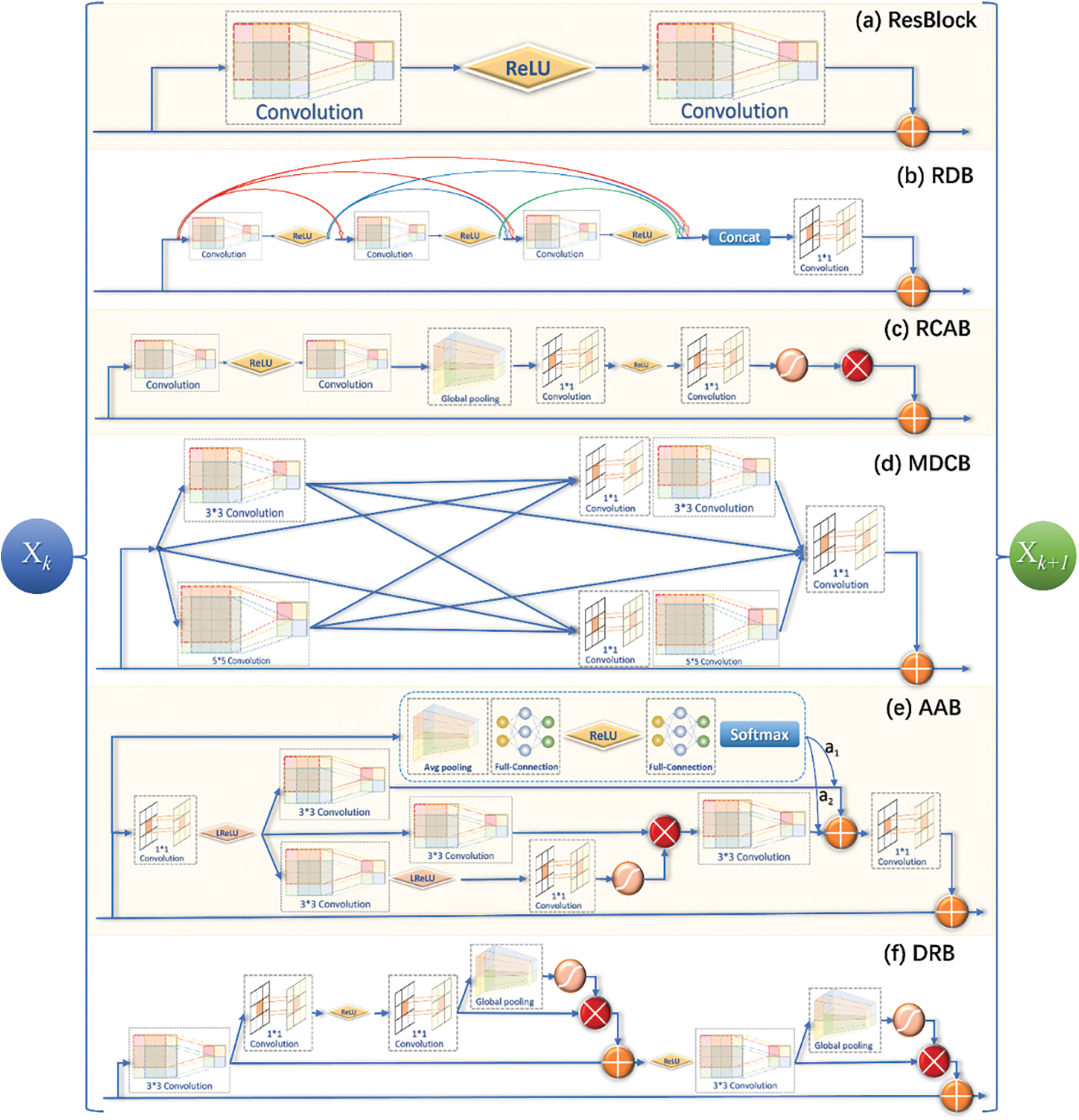
Figure 1: Common SR algorithm feature extraction modules (a) ResBlock for EDSR, (b) RDB for RDN, (c) RCAB for RCAN, (d) MDCB for MDCN, (e) AAB for AAN, and (f) DRB for MFFN

The EDSR network [15] uses the stacking of the ResBlock structure to extract the feature map, and although the removal of the batch normalization layer results in a performance enhancement, the width of the network becomes wider through increasing the channels of features. Although it helps to retain more features, the number of parameters strikingly increases. In RDN [16], the RDB structure is designed with residuals, and dense connections can extract richer feature information, but each stage in the RDB must fuse the previous features, which also increases parameters. In RCAN [17], the RCAB structure is designed to extract feature information by combining residuals and attention. In addition to the previously mentioned lack of pixel-based attention capability, there is a certain degree of information loss due to dimensionality reduction when generating the channel-based weight values. In MDCN [18], MDCB with different scale convolutions are designed for feature extraction to retain feature information to the maximum extent. MDCB extracts feature information using 3 × 3 and 5 × 5 convolutions, and then cross-fusion is utilized to obtain the final features, which retains more information and increases parameters.

The above analysis shows that the existing SR algorithms’ feature extraction structure mainly evolves through increasing channel count and convolution size and stacking more sub-modules to obtain more feature information, increasing the network’s parameter count and computing complexity. In addition, these SR algorithms’ feature extraction structures are static and cannot extract more differentiated information based on various inputs. Hence, further research is required to design lightweight and efficient feature extraction modules. Lightweight AI algorithms have been an active subject of research, and considering the real-life application of SR algorithms, lightweight SISR algorithms have been a commonly explored research pathway within the field of SR. Some lightweight networks have been proposed to improve the network speed while maintaining good accuracy, such as SqueezeNet [19], which achieves complete dimensionality reduction by 1 × 1 convolution and then extracts features by 1 × 1 and 3 × 3 convolutions before fusion to achieve the purpose of reducing the number of parameters. Inception [20] reduces dimensionality by 1 × 1 convolution while using multiple small-sized convolutions. The Xception [21] and MobileNet [22] series use deep separable convolution to significantly lessen the parameters and achieve good results. Hence, group convolution and depth-separable convolution are widely employed to achieve lightweight networks, and 1 × 1 convolutions are commonly employed in lightweight deep learning models to achieve expanded and reduced dimensionality.

Attention mechanisms can also help networks focus on helpful information for tasks and better utilize the correlation of input data. Therefore, it reduces the number of parameters while maintaining model performance, making the network more lightweight and efficient. AAN [23] combines the attention mechanism to design the AAN structure for feature extraction, and each extracted feature must be multiplied by a weight value, resulting in all channels using one weight for each pixel, which does not allow pixel-based attention capability. MFFN [24] proposed DRB with autocorrelation weight units (ACW) for image feature information extraction. The lightweight model can enhance image stripes effectively.

Based on the above research, lightweight SR algorithms such as CARN [25], AAN [23], and other lightweight SR networks have been continuously proposed. Although some of the above schemes can significantly reduce the network parameter count to improve the speed, in many cases, they still bring about a loss of accuracy. Excessive pursuit of network lightweight can also cause a decrease in the network’s learning ability, so how to design a reasonable network structure should also be considered based on actual needs.

This study first analyzes the feature extraction structures of different SR algorithms to design a more lightweight and adaptive feature extraction structure for SR algorithms. Inspired by the ideas related to dynamic convolution and attention mechanism, a lightweight adaptive feature fusion module AFB is proposed that achieves the differential extraction of feature information using dynamic convolution with scale information and combines the channel space of multi-feature fusion. The attention mechanism keeps significant feature information, and the pixel-based gating mechanism further enhances the module adaptivity, enabling the network to have stronger generalization and expression capabilities.

2  Method

2.1 Design of Lightweight Adaptive Feature Fusion Module

In most deep learning tasks, the feature extraction method directly determines the model’s performance. The feature extraction module, as the main component of the network, should be able to extract as much semantic information as possible while keeping it lightweight. At present, deep learning-based SISR algorithms use static convolutional kernels to extract feature information while seldom using the scale information of SR. This results in different input image information going through the same convolutional kernels to extract feature information, making it homogeneous. However, this method makes the reconstructed SR images inaccurate enough. A lightweight adaptive feature fusion module AFB (Adaptively-fusion Feature Block) for feature extraction was proposed to overcome these issues. In addition to combining dynamic convolution and attention mechanisms for the adaptive extraction of feature information and lightweight features, the AFB module can be used for fixed-scale SR tasks and arbitrary-scale SR. Fig. 2 shows the structure of AFB. GM (Gate Mechanism) is a pixel-based gating mechanism structure, DC (Dynamic Convolution) is a dynamic convolution structure combining scale information, and AB (Attention Branch) is an attention structure for multi-feature fusion.

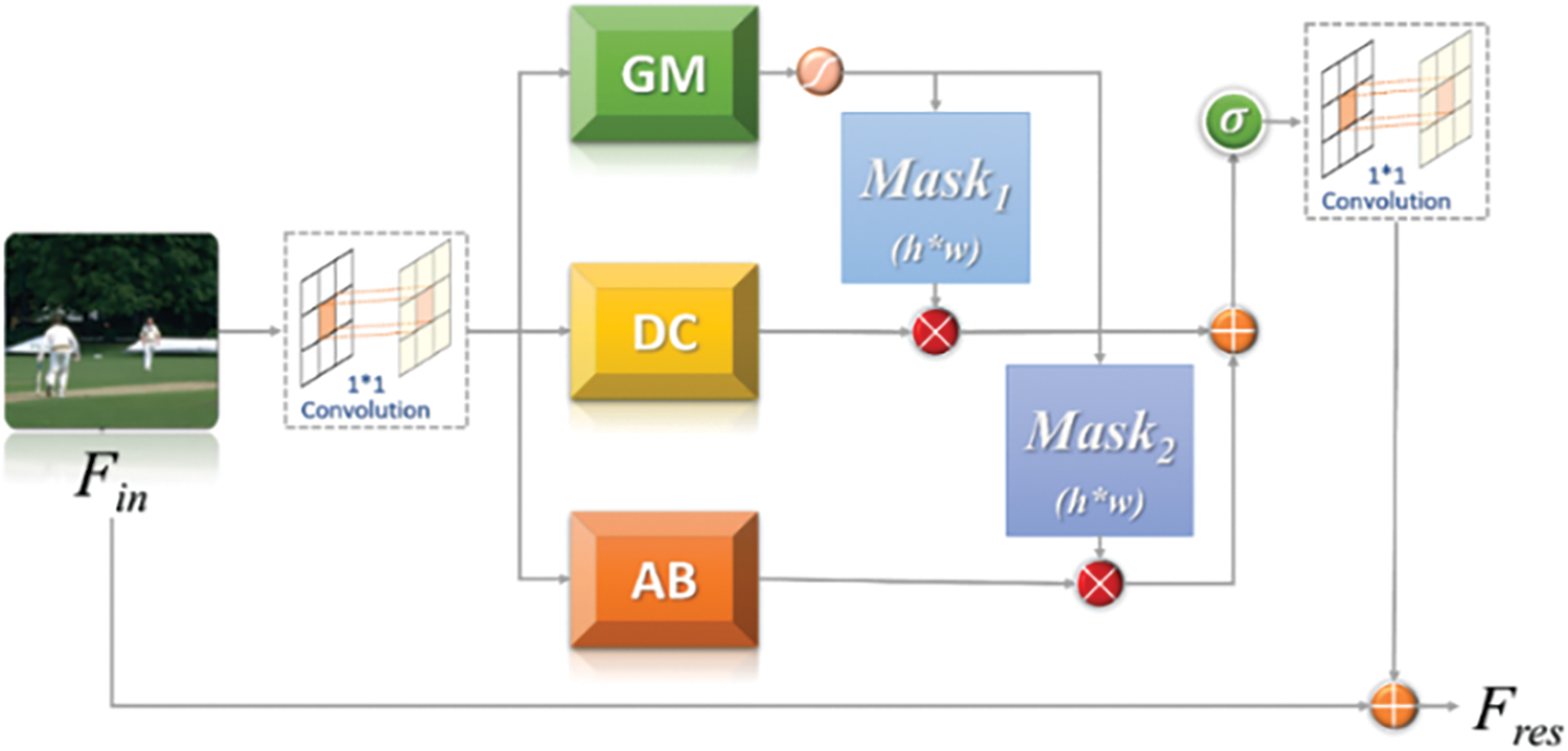
Figure 2: The structure of AFB (adaptively fusion feature block)

As an efficient feature extraction module, AFB can be easily used as a sub-structure in any network that requires feature extraction by stacking modules. The input features are employed as the input of GM, DC, and AB structures after 1 × 1 convolution and the GM structure outputs two h × w weight matrices after a sigmoid function. In the feature map, h is the height, and w is the width. The results of the multiplication of the DC and AB structures and the corresponding two weight matrices are added, and then the final adaptive feature map can be attained. Finally, it comes into the next stage after 1 × 1 convolution fusion. The execution flow is as follows. Fin in Eq. (1) represents the input feature map of AFB and Fout is the output feature map of it. The GM structure outputs two weight matrices, and the expressions are shown in Eq. (2).

Fout=HAFB(Fin)(1)

Mask1,2=σ(HGM(Hconv1(Fin)))(2)

where Mask1,2 is the two weight matrices of the output of the GM structure, both with the size of h × w. σ is the sigmoid activation function, Hconv1 indicates 1 × 1 convolution, and Fin is the current input feature. The detailed expression of the whole AFB module is shown in Eqs. (3) and (4).

Fmid=Mask1∗HDC(Hconv1(Fin))+Mask2∗HAB(Hconv1(Fin))(3)

Fres=Hconv1(σ(Fmid))+Fin(4)

where σ is the activation function, which is not necessarily sigmoid and can be chosen flexibly according to different needs, denotes the adaptive feature map, and Fres is the output feature map. Through the processing of AFB, the network can extract richer feature information, and the SR task helps the network to reconstruct more accurate high-resolution images. Fig. 2 depicts the structure of the AFB module, GM, DC, and AB, and each substructure is explained in detail below.

2.1.1 Dynamic Convolution Structure Combined with Scale Information

Dynamic convolution was first proposed by the Microsoft AI Cognitive Services team [26]. Static convolutions do convolution for different input images using the same convolution kernel, which lacks targeted feature extraction. Dynamic convolution combines multiple static convolutions and determines the parameters of dynamic convolution based on different input image information to improve expression capability. In this paper, the scale information is added to the original dynamic convolution for feature information extraction of multi-task scenes, and the improved dynamic convolution DC (Dynamic Convolution) structure in this study is as follows.

Fig. 3 indicates that x is first pooled by global averaging, and then a one-dimensional vector of length c (the channels count of the feature map) is obtained. After the obtained 1D vector of length c plus the scale information (which contains the length h and width w of the feature map. This is mainly aimed at SR tasks that require scale information to complete upsampling at any multiple. If used for fixed multiple SR or other feature extraction tasks, scale information can be removed) to generate a 1D vector of length c+2 after two full-connected layers and an activation function Rectified Linear Unit(ReLU) between them, as shown in Fig. 4.

Figure 3: The improved dynamic convolution structure

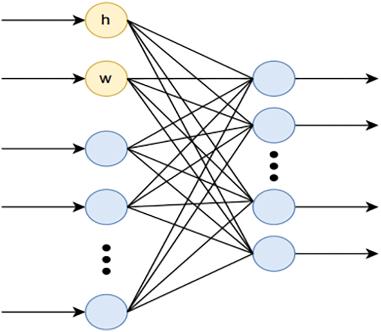
Figure 4: Full-connection layer

The number of full-connection layer neurons can be adjusted appropriately to optimize computational efficiency. h and w are mainly designed for the SR task that requires scale information to complete the upsampling, and these two parameters can be removed for other tasks. Adding the scale information and going through the two full-connection layers and ReLU, a 1D vector with n data (number of static convolutions) eventually yields, and Eq. (5) is the basic expression.

Fnext=H(a1∗conv1+a2∗conv2+…+an∗convn)(Fpre)(5)

where Fpre is the extracted feature information from the preceding layer, Fnext is the feature map after dynamic convolution, H(a1∗conv1+a2∗conv2+…+an∗convn) is the dynamic convolution, a1∗conv1+a2∗conv2+…+an∗convn means multiple static convolution multiplied by the accumulation of corresponding coefficients, and the result is the convolution kernel parameter of dynamic convolution, a1+a2+⋯+an=1. A better balance between parameters and performance can be achieved by setting the static convolution count n = 3 in the network. Dynamic convolution itself is designed for lightweight networks, which improves performance by increasing the number of channels or network depth, which significantly increases computational complexity. In inference, dynamic convolution performed through a linear combination of multiple static convolutions significantly reduces the computational complexity compared to increasing network depth and channel quantity.

2.1.2 Channel Spatial Attention Structure Based on Multi-Feature Fusion

Dynamic convolution can enhance the dynamics and adaptiveness of AFB module feature extraction in order to allow the AFB module to extract richer feature information. This study also introduces the attention mechanism in the AFB module, AB (Attention Branch) multi-feature fusion attention branch structure helps the AFB module extract high-frequency information from the feature map [19] while reducing or ignoring unimportant information. Fig. 5 shows the structure of the Attention Branch.

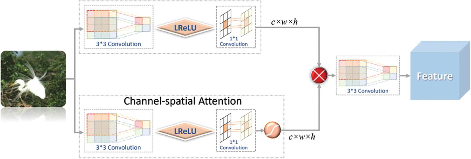
Figure 5: Attention branch

The input features are first extracted by the above 3 × 3 convolution and 1 × 1 convolution of the feature map) and used as input for the following channel space attention module. Finally, the two results are multiplied and then fused by 3 × 3 convolutions, and the final channel space attention feature map extracted by the AB module is obtained. The essential expression is shown as follows:

FAB=Hconv3(Hconv1(σ(Hconv3(Fin)))∗Hchannel−spatial(Fin))(6)

where Hchannel−spatial is the channel space attention, as shown in Fig. 5. When the input is c × h × w, c is the channels’ number of the feature map, h represents the height, and w is the width. After the 3 × 3 convolution and 1 × 1 convolution, the feature map is still obtained in the size of c × h × w, but there can be some unimportant information in the feature map obtained by this convolution that must be filtered. Hence, it is necessary to combine the channel attention to extract the essential information from the feature map. The following part of Fig. 6 depicts the channel space attention mechanism. Based on the input size, the size of the channel space attention weight is c × h × w, for example, c = 3, h = w = 3, and the two can be multiplied as shown in Eq. (6).

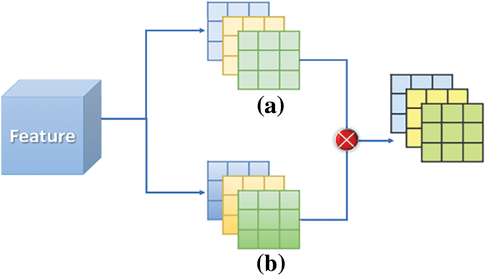
Figure 6: Schematic diagram of channel spatial attention. (a) Represents the feature map; (b) represent weight

After obtaining attention to feature maps through multi-feature fusion, more helpful information is preserved through 3 × 3 convolutional fusion. The AB structure and DC dynamic convolution structure extract the feature information of the previous layer, respectively, and then combine it with the GM structure to obtain the final AFB module feature map, as illustrated in Fig. 6.

2.1.3 Structure of the Pixel-Based Gating Mechanism

The addition of dynamic convolution makes the AFB module dynamic. A pixel-based gate mechanism structure GM (Gate Mechanism) is also proposed to enhance the self-adaptability of the AFB module. The GM structure generates two h × w weight matrices based on the feature information of the previous layer, where h is the height and w is the width of the feature map, which are assigned to the AB and DC structure extracted feature information, and is equivalent to the GM structure redistributing the importance of the feature information of AB and DC structures. Therefore, the combination of dynamic convolution and the GM structure makes the AFB module highly adaptive. It can adaptively extract the required feature information according to the input variability. The structure of GM can be understood in Fig. 7.

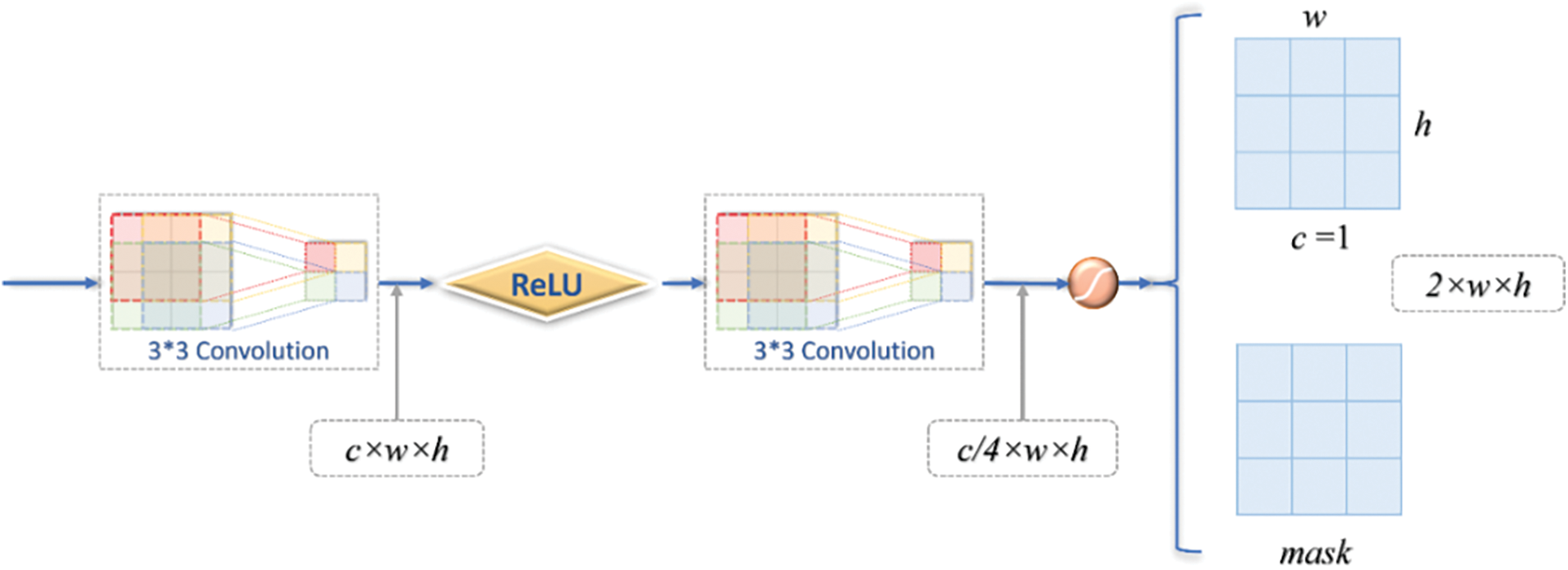
Figure 7: Gate mechanism

The GM implementation is shown in Fig. 7. The input features are convolved by two 3 × 3 and two activation functions to obtain two h × w × c weight filters mask, where c = 1, h is the height and w is the width, and the Sigmoid function scales the value of the mask to the interval of (0, 1), as expressed by the following equation:

Mask1,2=σs(Hconv3(σr(Hconv3(Fin))))(7)

where σr is the ReLU, σs is the sigmoid, and Mask1,2 is the matrix weights of the output, which can also be described as two weight filters. The GM structure determines which features per pixel of the output of the AB and DC structures are helpful at a particular stage and which are useless or less important. Re-enforcement by extracting important feature information helps to improve the network representation.

2.1.4 Analysis of Structural Features of Adaptive Feature Fusion Module

Through the previous research and analysis, the AFB module mainly consists of a dynamic convolutional structure with scale information, channel space attention structure with multi-feature fusion, and pixel-based gating mechanism structure, and the combination of these structures makes it lightweight, adaptive feature extraction and multi-task oriented. The lightweight design helps to reduce the model computation and inference speed so that the model can be deployed in practical engineering. The adaptive feature enables the model to have stronger generalization ability, consequently improving the robustness of the model.

Lightweight structure design: The AFB module is proposed based on the research and analysis of various feature extraction modules of the SR algorithm. The original intention of this design is that the network combined with the AFB module can effectively reduce the parameter number of the model while guaranteeing performance comparable to the current best algorithm. The number of covariates for its convolution is mainly calculated to reflect the advantages of the AFB module. Table 1 shows the specific comparison.

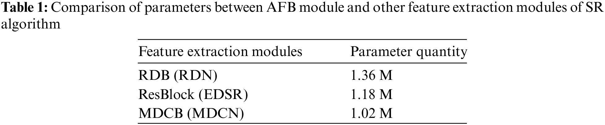
By combining the AFB module, the performance of this algorithm is competitive or even better than the other algorithms mentioned in Table 2, which explains the lightweight design of the AFB module compared to other SR modules.

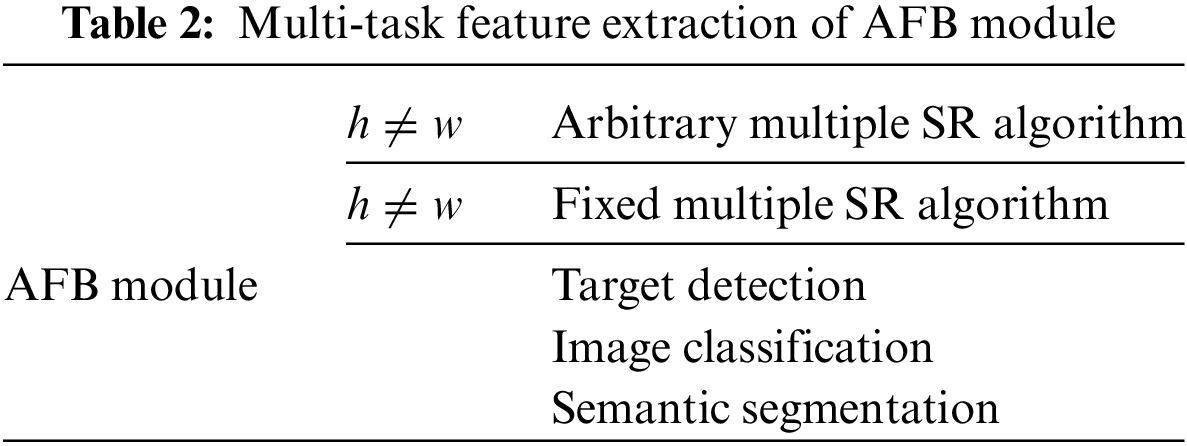
Multi-task-oriented feature: The AFB module can be applied to any network that requires feature extraction. When the scale scaling information h≠wis set in the AFB module, the AFB module can be used for any scale of the SR algorithm. When h≠w, it can be applied to fixed times of the SR algorithm, when the scale information is removed, it can be used for feature information extraction of vision tasks, as shown in Table 2.

Adaptive feature extraction: Except for the two traits mentioned earlier, the biggest advantage of the AFB module is the adaptive feature extraction capability. The dynamic convolution with scale information can extract differentiated information based on different input features, and the pixel-based gating mechanism GM module adaptively combines the feature information generated by the AB and DC structures through the two weight matrices generated, as shown in Fig. 2.

2.2 Validation Model Design Based on AFB Module

The AFB module of adaptive feature fusion can be oriented to multi-task adaptive extraction of feature information, and it can be used as a separate module integrated into other networks requiring feature extraction. The multi-feature fusion of channel space attention structure AB, dynamic convolution structure DC, and pixel-based gating mechanism structure GM can extract a richer feature map. A lightweight network AFBNet based on the AFB module is designed to evaluate its effectiveness. AFBNet is improved from Fast Super-Resolution Convolutional Neural Network(FSRCNN) [27,28], and the effectiveness of the AFB module is further demonstrated by comparing AFBNet and FSRCNN networks. FSRCNN achieves upsampling using deconvolution operations at the end of the network instead of interpolation upsampling at the front end, effectively reducing network computational complexity. At the same time, the newly proposed deconvolution structure has become the most commonly used upsampling method in super-resolution algorithms. This subsection first analyzes the characteristics of different upsampling methods, different loss functions of fixed multiplicity oversampling algorithms, and different degradation model principles and then designs the lightweight AFBNet network structure based on these.

2.2.1 Research and Analysis of Fixed Multiplier Upsampling Method

The fixed multiplier oversampling algorithm indicates that the designed oversampling algorithm can only achieve a certain fixed multiplier upsampling, and the current common fixed multiplier-based upsampling methods are interpolation upsampling inverse convolution, and subpixel convolution upsampling. The following is the analysis of the characteristics of each of the inverse convolution upsampling and subpixel convolution upsampling methods.

Inverse convolution upsampling: In FSRCNN, the upsampling module adopts the inverse convolution for the first time. Here, the inverse convolution operation ConvTranspose2d in the Pytorch deep learning framework is employed to illustrate, like the conventional convolution, the inverse convolution also includes the basic elements such as convolution kernel (kernel_size), stride, and padding. The definition of the convolution kernel size in the inverse convolution is the same as that of the conventional convolution, and the padding formula of the inverse convolution is as follows:

real_padding=kernel_size−1−padding(8)

Real_padding in Eq. (8) is the number of zero padding for deconvolution. When set padding = 0, it is the regular convolution. Meanwhile, if stride = 1, the size is reduced after convolution kernel_size-1. When the convolution result needs to be restored to its original size, padding = kernel_size-1 must be set. This is equivalent to the padding kernel_size-1 of regular convolution, and the size after convolution is the same as before, i.e., real_ padding = 0. The step size of deconvolution is no longer the meaning of step size in regular convolution but more like the meaning of step size in zero convolution. The step size of deconvolution is no longer the meaning of the step size of regular convolution but more like the hole rate of hole convolution. In the deconvolution, the original concept of step is at this time constant equal to 1, while the step in this study controls the gap between pixel points. For example, if stride = 1, the gap between pixel points is 0; when stride = 2, the gap is 1. These gaps are filled with zero, so the feature map size can be calculated given the step size, as shown in Eq. (9).

output=(input−1)∗stride+1(9)

Based on the above description of convolution kernel, step size, and padding in deconvolution, given the input feature size i, deconvolution kernel size k × k, step size s, and padding p, the output size can be obtained.

o={((i−1)∗s+1)+(k−1−p)∗2−k}1+1+outpadding(10)

o=(i−1)∗s−2∗p+k+outpadding(11)

Eq. (11) can be compared to the conventional convolutional (Eq. (12)), where p is multiplied by two because the padding is generally not just single-sided padding but either top and bottom or left and right.

o=(i+2∗p−k)s+1(12)

Eq. (11) also has out padding, but the padding is only to fix the size of the output feature map size, and not zero padding of the feature map after deconvolution out padding.

Fig. 8 shows the deconvolution calculation for k = 3, s = 2, and padding = 1. Based on the previous introduction, the deconvolution will complete the upsampling by padding zero, which will somewhat affect the reconstruction effect.

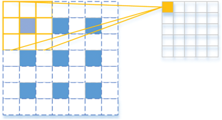
Figure 8: Schematic diagram of deconvolution

Subpixel convolution upsampling: Subpixel convolution, depicted in Fig. 9, achieves upsampling by increasing the number of channels of features to achieve pixel rearrangement. For example, for a 32-channel feature map, if it needs to be upsampled twice, the subsequent convolution needs to generate a 32 × 2 × 2 = 128-channel feature map, and then rearrange the pixels of every four channels into one channel to finally generate a 32-channel feature map of twice the original size.

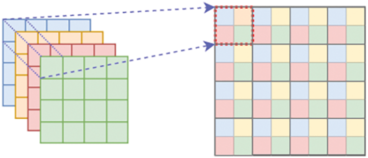
Figure 9: Schematic diagram of subpixel convolution

When upsampling is done twice, four channels are combined into one channel. Sub-pixel convolution is performed by combining individual pixels of a multi-channel feature map onto a new feature map unit pixel, and the original multiple feature map individual pixels can be considered as sub-pixels of the new feature map pixel.

2.2.2 Analysis of the Loss Function of the Super Division Algorithm

In SR algorithms, the customization of the loss function is crucial to complete the feedback propagation, calculate the gradient by determining the loss, and finally update the network parameters [29]. Several common loss functions of pixel-based SR algorithms are L1 loss function, L2 loss function, and Charbonnier loss [30], and the following is an analysis of the respective characteristics of pixel-based loss functions.

L2 loss function: L2 loss is also called mean-square error (MSE) loss, which is widely used in SR tasks, and the primary expression is as follows:

L2(I^,I)=1hwc∑i,j,k(I^i,j,k−Ii,j,k)2(13)

where hwc is the height, width, and channel number, I^ is SR, I is HR (Ground truth), and i,j,k is a pixel value.

L1 loss function: The L1 loss function, also called mean absolute error (MAE), is theoretically based on L1 with less computational effort compared to L2 loss, while the reconstruction effect of L1-based loss is generally better than L2-based loss, and its essential expression is as follows:

L1(I^,I)=1hwc∑i,j,k|I^i,j,k−Ii,j,k|(14)

Charbonnier loss function: It is proposed in LapSRN [31], based on L1 and L2 losses, considering only empirical risk minimization, which is prone to overfitting. LapSRN enhances the model’s generalization ability by incorporating a regularization term in the objective function, and the basic expression is as follows:

Lcha(I^,I)=1hwc∑i,j,k(I^i,j,k−Ii,j,k)2+ϵ2(15)

The loss functions mentioned above are the most commonly used pixel-based ones, which measure the loss by assessing the discrepancy between corresponding pixel values.

2.2.3 Study and Analysis of Different Simulation Degradation Models of the SR Algorithm

The image quality degradation process is very complex and generally results from a combination of different degradation causes. Image degradation may occur in hardware imaging systems, such as blurring from camera shake during image transmission or the poor environment in which the image was captured, which can also affect the image’s quality.

In deep learning-based SR algorithms, since it is challenging to get Low Resolution-High Resolution (LR-HR) image pairs in natural scenes, this study simulates the natural degradation process of existing HD images by combining several common degradation models to form LR-HR image pairs for supervised super-segmentation task training. The common methods for simulating degradation by SR algorithms are interpolation downsampling, blurring, noise, and JPEG compression.

Downsampling: Due to the high cost of obtaining image pairs of natural scenes, some degradation models often simulate the degradation process in natural scenes, and interpolation downsampling is the most commonly used degradation model in SR, including nearest neighbor, bilinear, and bicubic interpolation downsampling. Bicubic interpolation downsampling is the most frequently used method among them, and bicubic interpolation, also known as cubic convolutional interpolation [31,32], uses 16-pixel points around the sampling point P (P point is the location where the target pixel location is mapped to the original map) to perform bicubic interpolation, which is better than nearest neighbor interpolation and bilinear interpolation, but also increases the computational effort. The coefficients of each pixel point and the commonly used basis function formula are as follows:

y(x)={(a+2)|x|3−(a+3)|x|2+1,|x|≤1a|x|3−5a|x|2+8a|x|−4a,1<|x|<20,otherwise(16)

Based on Eq. 16, the following equation is derived when a=−1.

y(x)={|x|3−2|x|2+1,|x|≤14−|x|3+5|x|2−8|x|,1<|x|<20,otherwise(17)

The graph of the basis function according to Eq. (17) is shown below.

Fig. 10 shows the basis function for bicubic interpolation when a=−1. Once the value of parameter a is determined, the obtained basis function can be utilized to generate the weight values of 16 pixels around point P. Then, the multiplied product of pixel value and weight corresponding to each pixel point is summed to obtain the pixel value of the target image’s corresponding point, and the pixels’ location adjacent to point P is shown in Fig. 11. Black dots represent pixel position coordinate information.

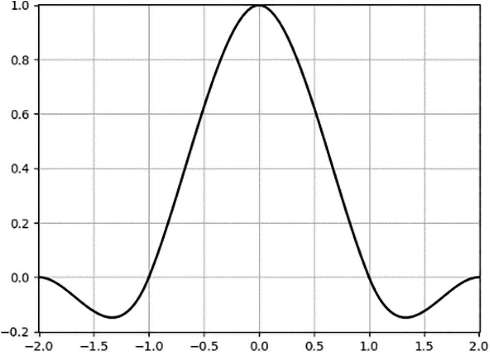
Figure 10: Specific graph of bicubic interpolation basis function when a=−1

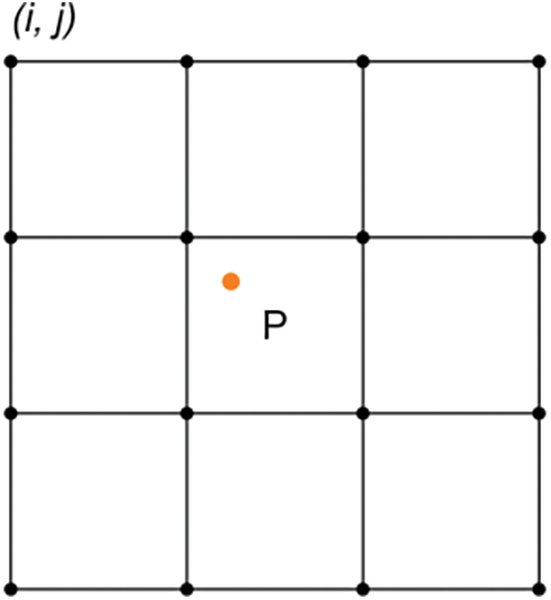
Figure 11: Pixel position adjacent to point P

Point P of Fig. 11 is the position of the corresponding point in the target image mapped to the initial image with the following mapping equation:

xsrc=xdstscale(18)

ysrc=ydstscale(19)

The target image point P(xdst,ydst) is mapped to the location P(xsrc,ysrc) of the original image according to the scaling multiple scale. The pixel value of P(xdst,ydst) can be obtained using Eq. (20).

P(xdst,ydst)=∑i=03∑j=03aij∗y(xi−xsrc)∗y(yj−ysrc)(20)

where aij is the pixel value of each pixel in the neighborhood, and y(xi−xsrc)∗y(yj−ysrc) is the weight at that point. It should be noted that the weighted pixel values can be outside the range of 0–255, so it is also necessary to finally limit the value of P(xdst,ydst) to the 0–255 interval.

Blur: Gaussian blur is the most commonly used blur degradation model [33]. Image blurring can also be called image smoothing, and common blurs are mean blur, median blur, and others. A simple understanding of Gaussian blur is to calculate a weight matrix for a pixel in its neighborhood and multiply it by the value of the corresponding pixel in that neighborhood to obtain the blurred value of the pixel. The two-dimensional Gaussian function obtains the weight matrix, and the neighborhood size must be specified. The one-dimensional Gaussian function is as follows:

f(x)=1σ2πe−(x−μ)22σ2(21)

where μ is the mean of x, σ is the standard deviation of x. Since the mean calculation considers the center point as the origin, μ=0, it can be obtained using Eq. 22.

f(x)=1σ2πe−x22σ2(22)

The expression of the 2D Gaussian function can be obtained from the 1D Gaussian function.

f(x,y)=12πσ2e−x2+y22σ2(23)

where x,y are the coordinate values relative to the origin, and the weight matrix of the neighborhood can be calculated using Eq. (23) combined with the relative coordinate values of the neighborhood pixels, as shown in Fig. 12.

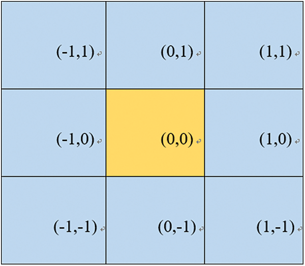
Figure 12: Relative coordinate values of pixels in the neighborhood

Noise: Gaussian noise is also a commonly used noise model. Gaussian noise uses Gaussian distribution to get the noise value summed to the original image, which can generate noise. In addition to Gaussian noise, it can add other noises, such as Pretzel noise, Rayleigh noise, and Uniform noise.

JPEG compression: JPEG compression is a loss compression method commonly used in digital images. The general method is first to convert the color space of the original image (such as to YCbCr space and others), then divide the image into small blocks of 8 × 8 for DCT transformation, and then perform quantization operations on the transformation coefficients, and others [34].

2.2.4 Network Structure Design of Verification Model Based on AFB Module

To validate the effectiveness of the AFB module, a lightweight network AFBNet based on the AFB module is designed for comparison experiments with the improved FSRCNN network. The architecture of the AFBNet network is shown below.

Fig. 13 indicates that the AFBNet network first goes through a 5 × 5 convolution for an input image. The 5 × 5 convolution has a larger view field and can extract more information, and the d-channel feature map can be obtained by the 5 × 5 convolution; here, d = 56, the following (Eq. (24)) is the expression:

Fd0=σ(Hconv5∗5(Fin))(24)

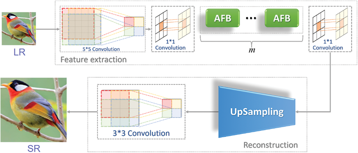
Figure 13: The architecture of AFBNet

Fin in Eq. (24) indicates the input feature map, size c × h × w, usually channel c = 3, H and W are the width and height of the image, Fout is the feature map of d × h × w obtained after 5 × 5 convolution operation and activation function, channel d = 56, σis the Parametric Rectified Linear Unit (PReLU) [35] activation function. The feature map of channel d is obtained after 5 × 5 convolutions. In order to obtain faster inference speed, the channel must be dimensionalized. As introduced in the previous section, dimensionality reduction or dimensionality expansion is generally achieved using 1 × 1 convolution. Channel d is obtained after 1 × 1 convolution, and then the feature map of channel s is obtained, where s is much smaller than d. The expression is as follows:

Fs0=σ(Hconv1∗1(Fd0))(25)

The obtained s-dimensional feature map is then passed through the AFB module to complete the feature mapping, where the number of AFB modules is set to m. After multiple AFB modules, the network can extract more useful feature information to reconstruct a clearer SR image with the following expressions:

Fs1=σ(HAFB(Fs0))(26)

After completing the feature mapping, the s-dimensional feature map is expanded to d-dimensions using a 1 × 1 convolution.

Fd1=σ(Hconv1∗1(Fs1))(27)

Expanding the dimensionality of the feature map can obtain richer feature information, then upsampling the d-dimensional feature map and fusing it by 3 × 3 convolutions. The final output feature map is derived with the following basic expressions.

Fout=Hconv3∗3((Hupsample(Fd1)))(28)

Fout in Eq. (28) is the output feature map, size C × H × W, generally C = 3, Hupsample for the upsampling operation, and the obtained feature map Fout can be displayed through post-processing. Through previous research and analysis of upsampling methods and different loss functions, the AFBNet and FSRCNN networks have used sub-pixel upsampling methods. The model was trained using the L1 loss function and simulated degraded image LR using bicubic interpolation.

3  Result

3.1 Datasets

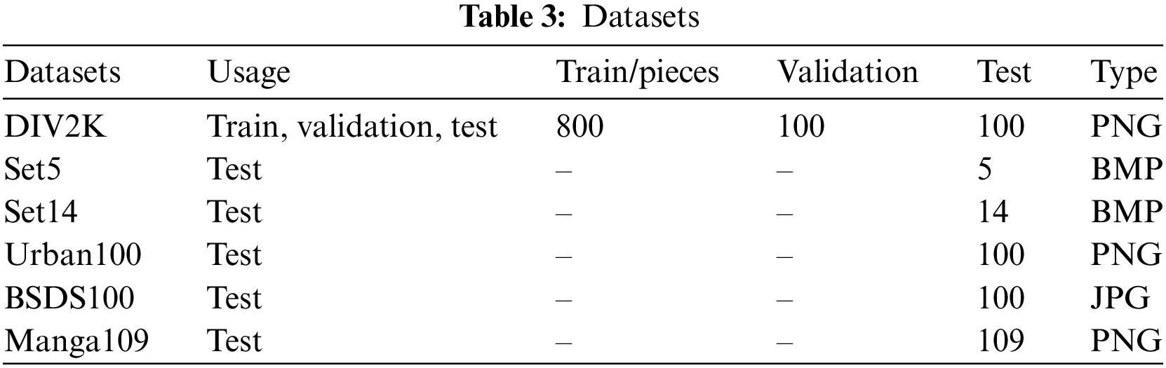
The super-resolution algorithm dataset is mainly divided into three categories: the sets for training, validation, and testing. This study mainly used the DIV2K [20] dataset for training. It is the most widely utilized dataset for training super-resolution algorithms. Tests are conducted using the Set5 [36], Set14 [37], Urban100 [38], BSDS100 [39], and Manga109 [40] datasets for test comparison. Set5 and Set14 are the primary test datasets for super-resolution algorithms. In the early stages of developing deep learning-based super-resolution algorithms, these two test datasets are mainly employed to compare the reconstruction effects. Urban100, BSDS100, and Manga109 are also commonly used datasets. Table 3 displays the detailed information of these datasets.

3.2 Dataset Process

Although a considerable number of training datasets are provided, the size of each image is relatively large and cannot be employed directly to train deep learning models in general. The difference between the input size required for training and the size of the original samples is significant, and direct use reduces the utilization of the original data information so that the trained model does not perform well. Hence, some processing of the datasets is required, as shown in Fig. 14.

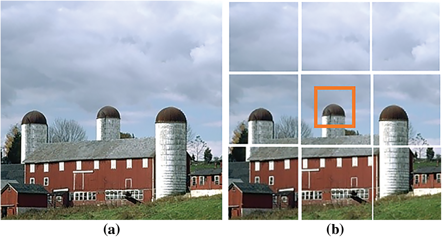
Figure 14: Training image clipping scheme. (a) The original data sample; (b) The small orange box is the training sample obtained by actual random clipping

Considering the DIV2K dataset as an example, it contains 800 high-definition images for training, 100 test images, and 100 validation images. If the train images are directly fed into the network for training, it will waste data resources and poor performance of the trained network. Some measures are considered to achieve better usage of all the information in each image: First, each image is cropped into a smaller size; for example, an image of 1920 × 1920 pixels is cropped into 16 images (480 × 480), through this operation can increase the training data set. If the 800 pieces of DIV2K training images are cropped into small images of 480 × 480 pixels, 32096 pieces of training images can be obtained. During the actual training, the network input images are smaller than those of 480 (480 pixels). Therefore, when the actual training is done, a randomly cropped fixed size on the 480 × 480 pixels image is used as the network input, such as 50 × 50 pixels and others. Introducing random cropping is equivalent to further expanding the dataset. Noise and blurring are usually introduced in the dataset to make the model more robust.

The training data process is shown in Fig. 15. In addition to cropping the original dataset to enrich the training set, getting a suitable LR-HR image pair is also essential. If the corresponding position information of HR and LR deviates too much, the model’s training and final performance will be significantly affected. For example, when training a 2-fold oversampling model, the HR image must be downsampled twice to get the LR, and the downsampling is generally done by bicubic interpolation downsampling. The width and height of HR should be even, and when it is odd, the SR obtained by downsampling and then upsampling will not be consistent with the original HR size. For the reconstruction of 4-fold oversampling, it should be noted whether the HR image is downsampled twice in succession by 2-fold or once by 4-fold. The experiment shows that two successive 2-fold downsampling will significantly affect the model’s performance because more information is ignored. Therefore, it can be concluded from the above that for an arbitrary number of times of oversampling, the pairs of images in each Batch_size should be set to the same size and the same downsampling times, and the downsampling of each HR image should be done once, instead of taking multiple consecutive downsampling.

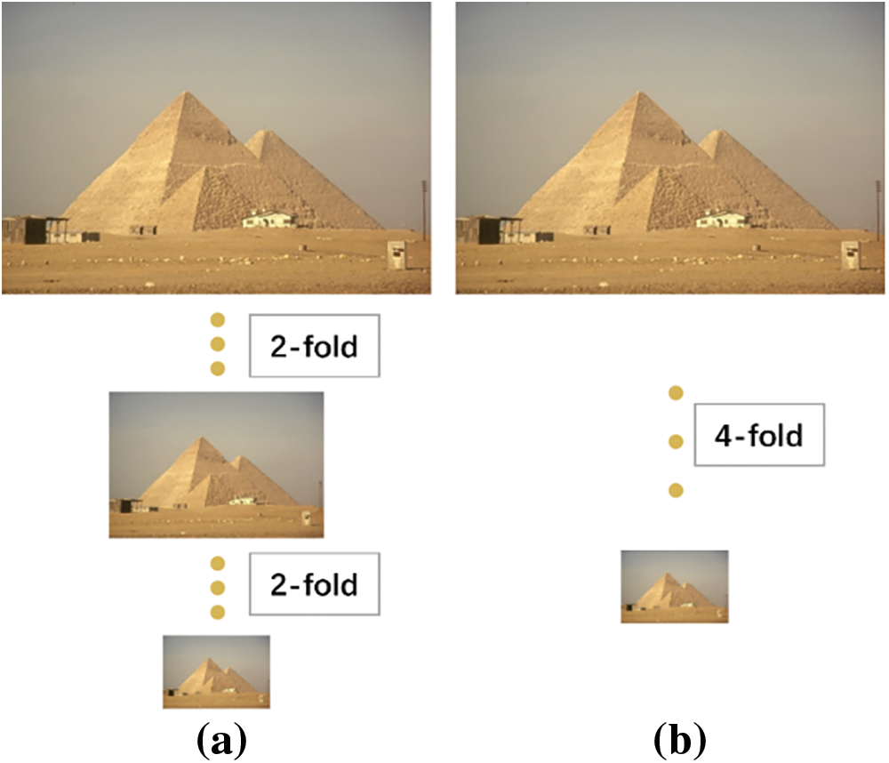
Figure 15: Schematic diagram of training data processing for four times super score. (a) Depicts continuous downsampling, (b) represents one downsampling; Better results can be achieved using method (b)

The above illustrates how to process the data set required for training to ensure the maximum utilization of the data, and it is also worthwhile to pay attention to how the processed data is loaded into the network for training. In general, the images can be loaded directly from the training data storage path for training, but the training process will take more time to load the data, and there may be insufficient memory, so the processed training data can be converted into h5py files first. h5py files have the characteristics of fast reading speed, high compression rate, and large data storage so that they can read more data than memory. In Python, the h5py format dataset is relatively simple to use, and it mainly consists of two containers: dataset (dataset) and group (group). The creation of h5py files consists of four main steps.

1) Create the h5py object.

2) Create different groups for the h5py object and name them.

3) Store the read data in each created group and set the corresponding index for easy reading.

4) Close the h5py file.

The steps to read the h5py file are as follows:

1) Open the h5py file.

2) Select different groups to get the corresponding data according to the index.

3) Close the h5py file.

These are the steps of reading and writing h5py files. Through the above description, the processing of training datasets in this study can be roughly grouped into the following processes, as shown in Fig. 16.

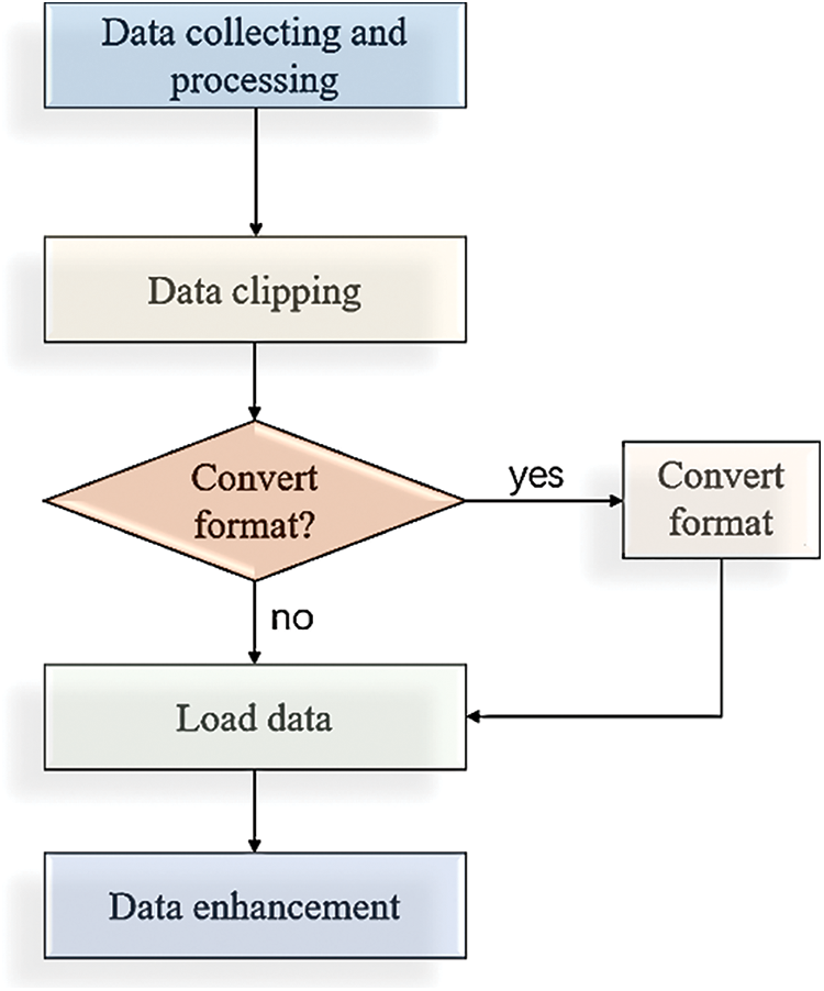
Figure 16: The processing flowchart of training data

Training parameters description and configuration: The training parameters also affect the final performance. The training parameters configuration mainly describes several vital parameters: optimizer selection, batch size, and learning rate size. When the learning rate is set and the gradient is found, the model parameters can be updated based on the optimizer to obtain the optimal solution. Today’s commonly used optimizers are SGD, Adam optimizer, RMSprop, AdaMax, and Nadam. This experiment mainly uses the Adam optimizer. Adam is an adaptive learning rate optimization algorithm called Adaptive Moment Estimation [41]. It will calculate the adaptive learning rate for each parameter to ensure the learning and updating of all parameters differentially, which is beneficial to speed up the network training. The specific formula is as follows:

mt=β1mt−1+(1−β1)gt(29)

ut=β2ut−1+(1−β2)gt2(30)

where gt is the current gradient, ut is the average of the historical squared gradients of exponential decay, and mt is the average of the historical gradients of exponential decay, similar to the momentum of the gradient descent method. When ut and mt are initialized as 0 vectors, the authors of Adam found that they are both biased towards 0, especially when the initialization and decay rates are low, such as when β1 and β2 tend to 1. The following bias correction offsets the bias.

m^t=mt1−β1t(31)

u^t=ut1−β2t(32)

Based on Eqs. (31) and (32), the updated rules of Adam are as follows:

θt+1=θt−ηu^t+ϵm^t(33)

where β1 can be set to 0.9, β2 can be set to 0.999, ϵ=10e−8. Based on practical experience, Adam performs better than other adaptive algorithms. Generally, a large Batch_size helps to move in the direction of a more accurate gradient. However, it is not easy to jump out when encountering saddle points, while a small Batch_size is more volatile and lacks stability, but at the same time, helps to jump out of the minimal value, so it is necessary to adjust Batch_size continuously based on the actual situation to ensure proper convergence. The learning rate changes synchronously with Batch_size. When Batch_size increases, the learning rate also increases by a corresponding multiple.

The basic experimental parameters setting: The input size of the training image is 50 × 50, the learning rate is 5e-4, and is halved every 50 iterations, Batch_size = 16, the iterations’ number epoch = 200, the optimizer selects adam, the loss function is L1 loss, the training data set is DIV2K, the test sets are Set5, Set14, Urban100, BSDS100 and Manga109, with upsampling multipliers of 2x and 4x. For each input image, the data is enhanced by utilizing a 90°rotation, horizontal and vertical flip, and the test images are still transformed into YCbCr color space and tested on their Y channels. The graphics card configuration in the experiment was RTX3090, and the training lasted about 20 h.

3.3 Evaluation Metrics for Super-Resolution Algorithms

Peak signal-to-noise ratio (PSNR): PSNR is the most commonly used evaluation method in the SISR algorithm, mainly obtained by calculating the mean square error (MSE) between SR and HR to determine the final result. It can be calculated using Eqs. (34) and (35).

MSE=1HW∑i=0H−1∑j=0W−1(IHR(i,j)−ISR(i,j))2(34)

PSNR=10∗log10(MAX2MSE)(35)

where H and W are the height and width of the image, (i,j) are each pixel point. MAX is the maximum pixel value in the image, such as MAX = 255 in a grayscale image. Eq. (35) indicates that the calculation of PSNR is highly correlated with MSE, so the super-resolution model trained on the loss function of MSE has more advantages in PSNR calculation. In addition, the results obtained from PSNR calculation cannot fully reflect the quality of image reconstruction. PSNR computation only targets a single pixel in two images, and the obtained results also show pixel differences between independent pixels. Therefore, the correlation between pixels in the image is not considered.

Structural similarity ratio (SSIM): SSIM is also commonly employed to evaluate the similarity between two images. Considering that in super-resolution tasks, the quality of SR reconstruction must be evaluated by comparing the overall similarity between SR and HR images, SSIM multidimensional calculation is naturally a good choice. In SSIM calculations, the differences in structure, luminance, and contrast between two images should be calculated.

SSIM(x,y)=(l(x,y)α⋅c(x,y)β⋅s(x,y)γ)(36)

α>0,β>0,γ>0, x represents SR, y represents HR.

l(x,y)=2μxμy+c1μx2+μy2+c1(37)

c(x,y)=2σxy+c2σx2+σy2+c2(38)

s(x,y)=σxy+c3σxσy+c3(39)

where l(x,y) is luminance comparison, c(x,y) is contrast comparison, s(x,y) is structural comparison, μx,μy is the mean value of x,y, σx,σy is the standard deviation of x,y, σxy is the covariance of x,y, c1,c2,c3 are constants to avoid situations where the denominator is zero. SSIM has symmetry: SSIM (X, Y) = SSIM (Y, X). SSIM is in the interval [0, 1], and a larger value indicates better reconstruction quality. The calculation of SSIM consists of three parts. Compared to PSNR, which only considers the difference between individual pixels, SSIM better considers the intrinsic correlation between pixels. It is more reasonable to comprehensively evaluate the similarity between the two images by combining the brightness, contrast, and structure of the two images.

3.4 AFB-Based Validation Model Ablation Experiment

Based on the previous study, the content of this subsection mainly verifies the role and advantages played by each substructure of the AFB module through ablation experiments. In the AFB module, the DC, AB, and GM structures greatly enhance the module’s adaptive feature extraction capability. This section designs a comparison experiment between the AFB module feature extraction scheme using the DC structure and the AFB module feature extraction scheme based on ordinary convolution to confirm the advantages of the DC structure in the network. The experiments keep the same configuration as the previous basic configuration except for the changes to the specified structure. The experiments in this subsection only verify the advantages of each sub-structure of the AFB module.

Analysis of DC structure with scale information: In order to validate the advantage of the AFB module for feature extraction, this section designs a lightweight AFBNet network based on the AFB module and FSRCNN network, and the effectiveness of the structure is verified by comparing the test results of whether DC is added to the AFBNet network or not. The experiments are conducted under a 4-fold fixed multiplicity superfraction task with 200 epochs of iterations and a test dataset of Set5.

The test indicated that the AFBNet network incorporating the DC structure improves its PSNR value by about 0.1 dB, which also verifies the effectiveness of the DC structure in AFBNet, as shown in Fig. 17. The DC structure is mainly employed to extract the differentiated feature information, as depicted in Fig. 18.

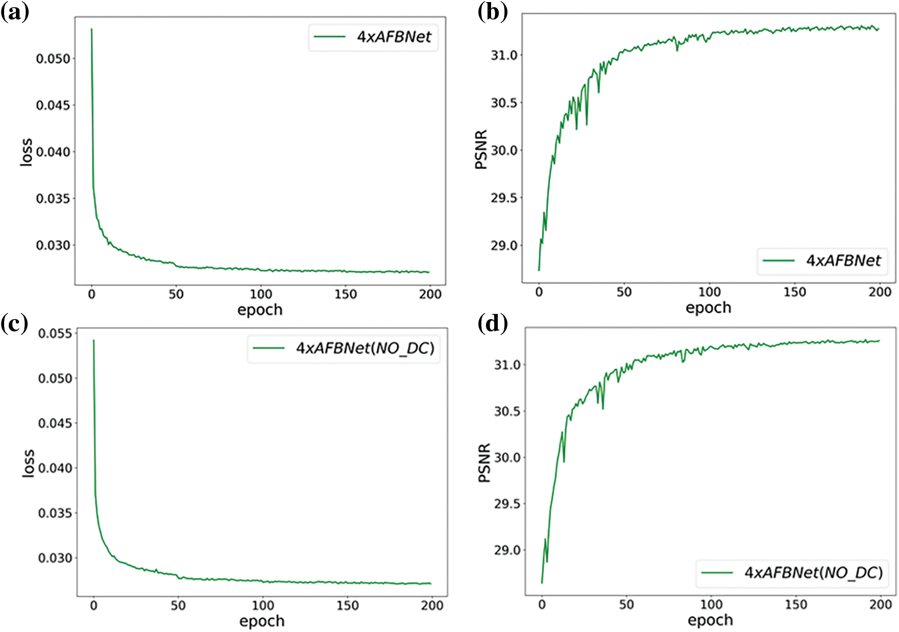
Figure 17: AFBNet training results under four times super score. (a) and (b) are AFBNet network training losses and PSNR values; (c) and (d) are the loss and PSNR values of the AFBNet network without adding dynamic convolution DC

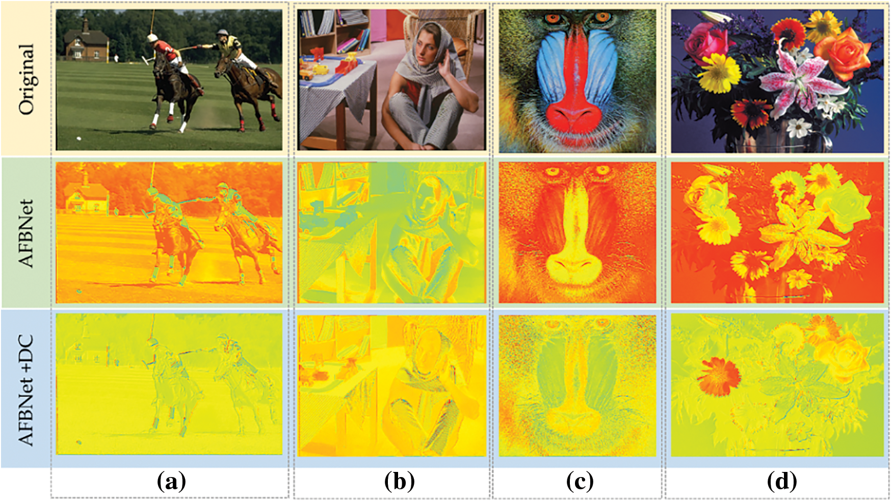
Figure 18: Thermodynamic diagram comparison of feature information extracted by AFBNet. (a), (b), (c), and (d) columns are thermodynamic diagram comparisons of feature information of the AFBNet network with and without DC structure. The 1st row is the original picture display; The 2nd row is the thermodynamic diagram of the output feature maps of the 4th AFB module without DC structure; The 3rd row is the thermodynamic diagram of the output feature maps of the 4th AFB module with DC structure

The heat map implementation shown in Fig. 18 must first get the feature maps of the input image through the fourth AFB module of the AFBNet network and then collect the feature maps of all channels to have the final heat map. Fig. 18 indicates that the general style of the heat map of the feature information extracted by AFBNet without DC structure is similar, whether the information in one or different images is not differentiated enough. The heat map produced by the network with dynamic convolution (DC) structure shows more apparent variations, especially when flowers are displayed in column (d). It effectively captures distinctions in color and features among the flowers. In contrast, the heat map generated by AFBNet without the DC structure exhibits less variation and fails to distinctly represent differences in color and features across the flowers. Through the above experiments, the DC structure can effectively enhance the generalization and expression ability of the network and realize the differentiated extraction of feature information for different input image information.

The AB structure can extract high-frequency information in the image using the channel space attention mechanism, which further enhances the expression ability of the network. The effectiveness of the structure is verified here by comparing the test results of the AFB module with the AB structure incorporated and the AFB module with the AB structure replaced by a common 3 × 3 convolution. The experiments are still conducted under a 4-fold fixed multiplicity superfraction task with 200 epochs of iterations and a test dataset of Set5.

The above experiments mainly verified the role of the AB structure in network performance improvement, and more high-frequency information about image features that the AB structure can obtain is still demonstrated by the heat map. Fig. 19 exhibits that adding AB structure with multiple feature fusion significantly improves the performance of the AFBNet network with a PSNR improvement of 0.12 dB. The AB structure highlights the important high-frequency information in the features compared to the ordinary convolution, while the multiple fusion of features also ensures the richness of feature information.

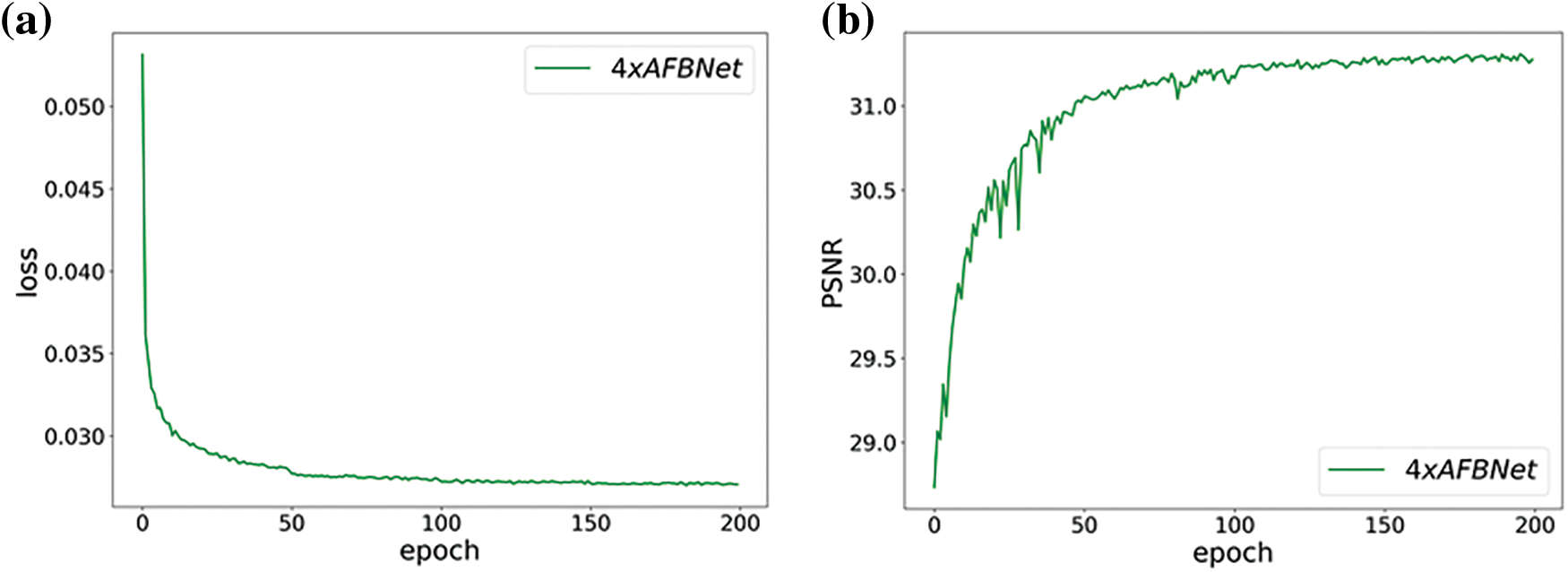
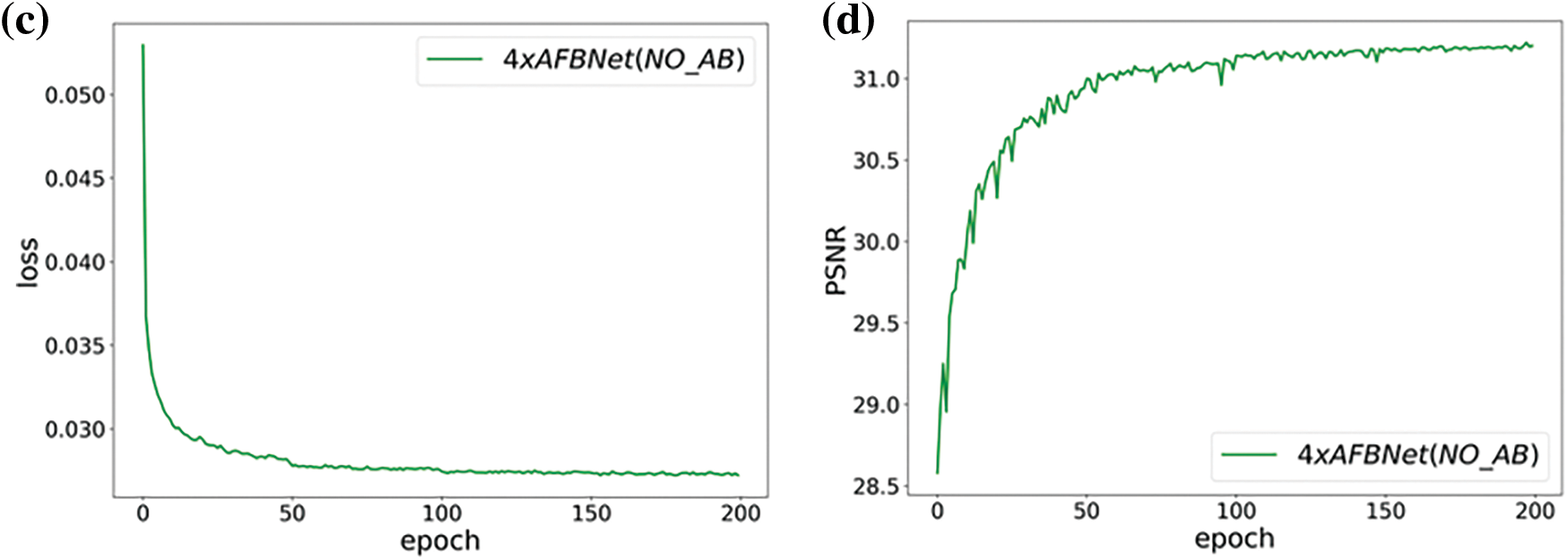
Figure 19: AFBNet training results under four times super score. (a) and (b) are AFBNet network training losses and PSNR values; (c) and (d) are the training loss and PSNR value of AFBNet network without AB structure

Fig. 20 shows that the inclusion of AB structure enables the network to extract more high-frequency information, which is conducive to the reconstruction of a higher-definition image. Column (d) of the figure shows that the high-frequency information of the thermodynamic feature map extracted by the AFBNet network without the addition of the AB structure is not rich enough, and the overall display of the image is not sharp enough. Meanwhile, the thermodynamic feature map of the feature information extracted by the AFBNet network, along with the addition of the AB structure, has more precise details and distinct edges. The above experiments prove that the AB structure can extract high-frequency information.

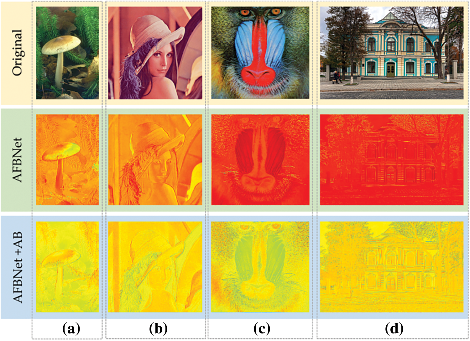
Figure 20: Thermodynamic diagram comparison of feature information extracted by AFBNet network. (a)–(d) columns compare feature information extraction of AFBNet networks with and without AB structures. First, input the original image of the network as a comparison. The 2nd row is the thermodynamic feature map extracted by the 4th AFB module when the AB structure is not added. The 3rd row is the thermodynamic feature map extracted by the 4th AFB module when AB structure is not added

Analysis of the pixel-based gating mechanism structure GM: The GM structure automatically generates two weight matrices by inputting feature information. Considering that the feature details extracted by the AB and DC structures do not necessarily have the same importance. The GM structure adaptively assigns weights to each pixel of the feature map for each channel using the two weight matrices to make the network structure more adaptive. The validity of the structure is demonstrated by comparing the test results of the AFB module with and without including the GM structure. The experiments are still performed under a 4-fold fixed multiplicity superfraction task with 200 epoch iterations and a test dataset of Set5.

Fig. 21 shows the experimental training results. Adding the GM structure improves the PSNR value of the network by 0.13 dB, depicting the effectiveness of the pixel-based gating mechanism module GM. The following mainly illustrates the adaptive feature extraction capability of the GM module.

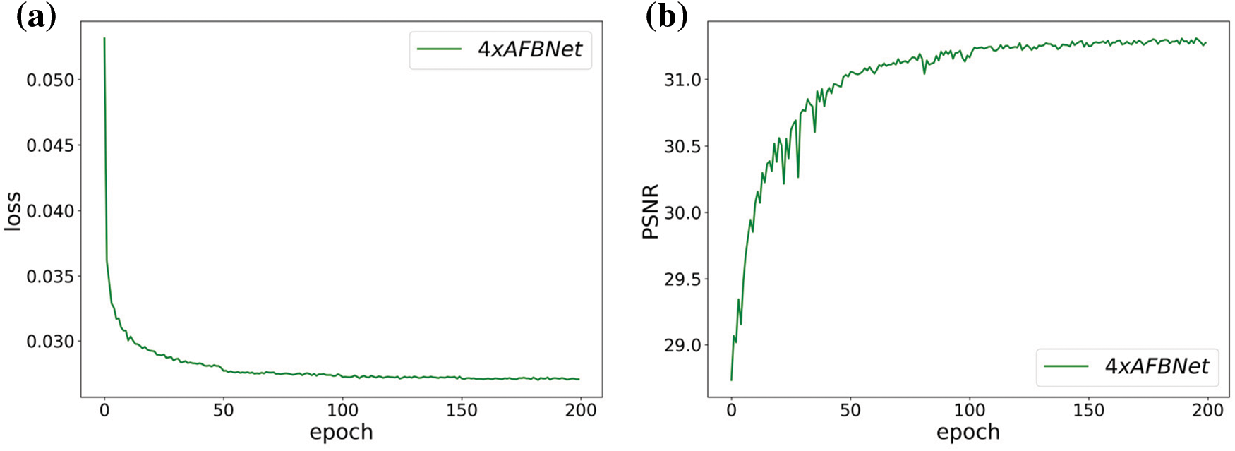
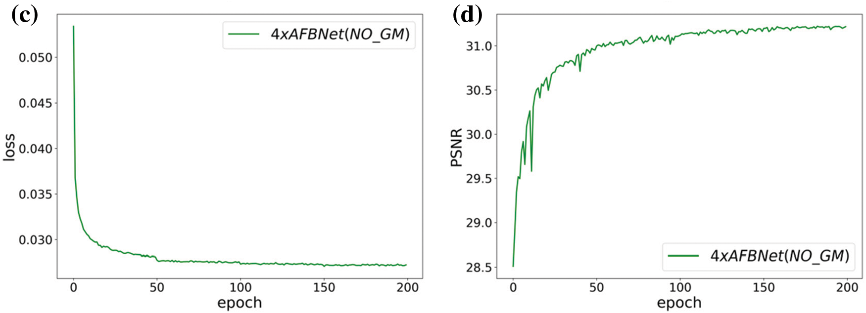
Figure 21: AFBNet training results under four times super score. (a) and (b) are AFBNet network training losses and PSNR values; (c) and (d) are the training loss and PSNR value of the AFBNet network without adding GM structure

Fig. 22 indicates that the characteristics of the feature maps obtained by directly adding the AB structure and DC structure are not obvious enough, and the overall information of the image is not expressive enough. The results obtained using the GM module to combine the feature information of AB and DC are more accurate, reflecting the adaptive characteristics of the GM module.

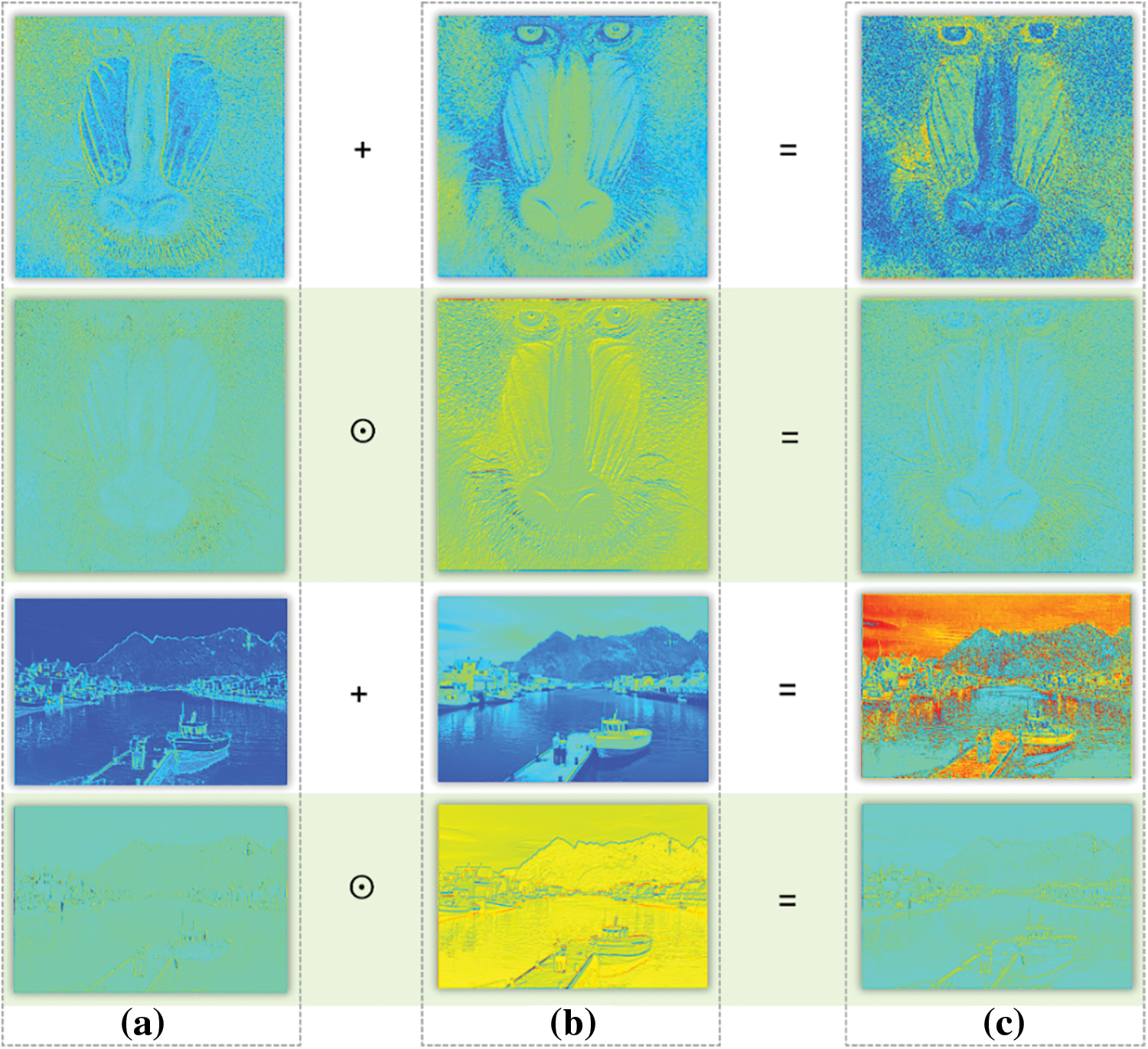
Figure 22: Comparison of thermal maps of feature information extracted by AFBNet network, (a)–(c) are the three columns of thermal maps of the AB structure, DC structure, and the combined feature map extracted by the AFBNet network, respectively. The plus sign indicates the feature map obtained by adding the two directly; the symbol ⨀ represents the feature map obtained by combining AB and DC through the GM structure

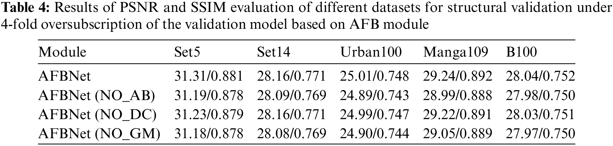
Table 4 shows that the AFB module mainly consists of three structures, AB, DC, and GM, each of which is an integral part. The advantages of the AB structure are illustrated by testing the changes in PSNR and SSIM values with or without the AB structure under different test datasets. The advantages of DC structure are illustrated by testing the changes of PSNR and SSIM with or without DC structure under different test datasets. In addition, the advantages of GM structure are demonstrated by testing the changes of PSNR and SSIM with or without GM structure under different test datasets. The experimental data show that each of the structures of the proposed AFB module is effective, and the combination of these structures can lead to further improvement in the expressiveness of the network.

3.5 Comprehensive Experimental Comparison and Analysis

Based on the previous basic configuration, the upsampling multiplier of the AFBNet network and the modified FSRCNN network is set to 2, and the test set is Set5. The test sample is edge-cropped to 2 pixels on all four sides for 200 training sessions, the HR image is downsampled for bicubic interpolation, and the LR image is obtained by downsampling two times at once. Then, the training sample of the input network is derived by random cropping, and the training visualization results are as follows:

Fig. 23b shows the AFBNet network based on the AFB module, which fluctuates more at the beginning of training. It also indicates that the AFB module must learn more but is stable after a learning period. Fig. 23d exhibits that FSRCNN is easier to learn due to its uncomplicated design, and the whole training process is smoother. Fig. 23c demonstrates that the loss decreases significantly every 50 times, which is because the learning rate is set to halve every 50 times, while the loss decreases no longer significantly after 150 times, which also reflects that the training tends to saturate. By analyzing the FSRCNN and AFBNet networks, it can be observed that incorporating the AFB module can significantly improve the network’s expression ability. Table 5 shows the specific test data.

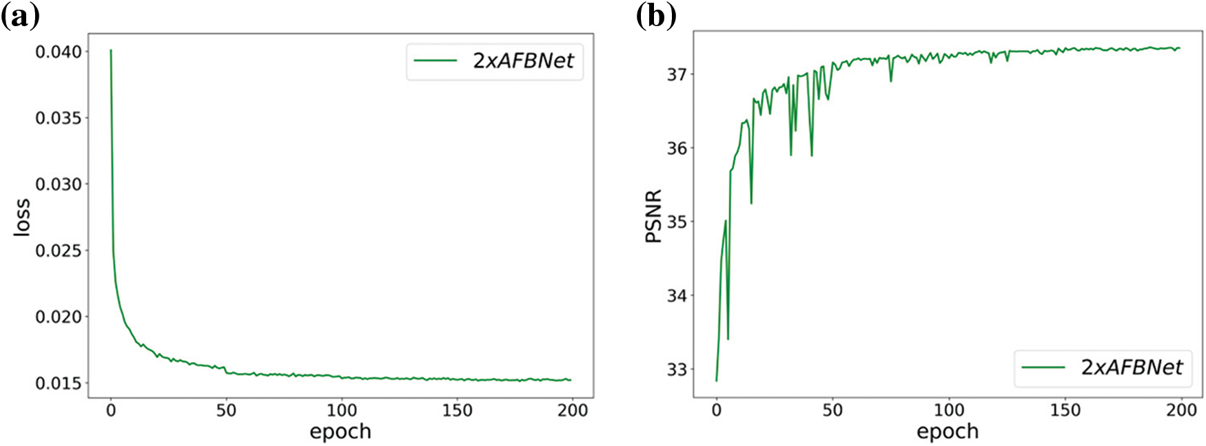
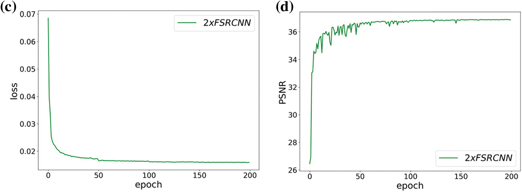
Figure 23: Training results of FSRCNN and AFBNet under 2-fold overscoring. (a) and (b) show the training loss and PSNR values of the AFBNet network; (c) and (d) show the training loss and PSNR values of the improved FSRCNN network

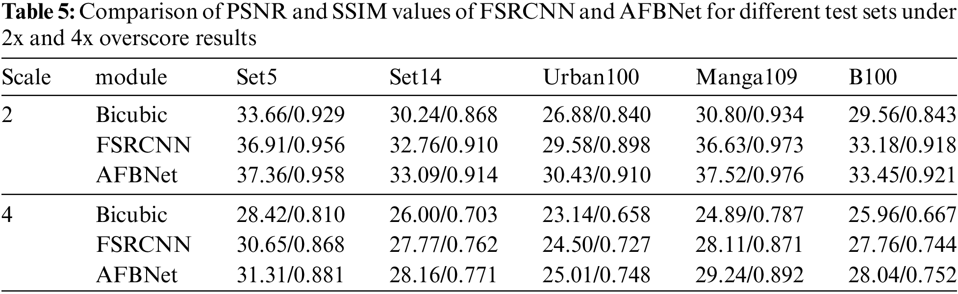
Fig. 24 depicts the training results of the FSRCNN and AFBNet networks under the div2k training dataset with 4-fold overscoring and the test dataset using Set5. Fig. 24 shows that the peak signal-to-noise ratio of the AFBNet network incorporating the AFB module is also substantially improved compared to the improved FSRCNN. The PSNR and SSIM values of FSRCNN and AFBNet networks under different test sets are tested based on the 2- and 4-fold SR models obtained from the training.

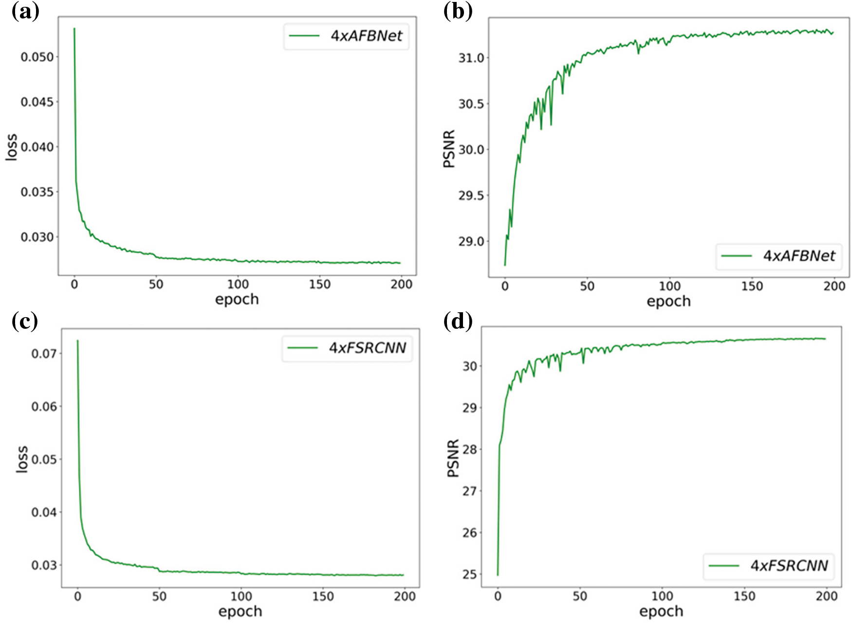
Figure 24: Training results of FSRCNN and AFBNet under 4-fold overshoot. (a) and (b) show the training loss and PSNR values of the AFBNet network; (c) and (d) indicate the training loss and PSNR values of the improved FSRCNN network

Table 5 indicates that comparing the PSNR and SSIM values of the improved FSRCNN and AFBNet networks under different test sets and incorporating the AFB module can help the network extract more helpful information for SR reconstruction. Although the AFB module slightly increases the number of parameters, it improves the model’s performance more, and this experiment further demonstrates the effectiveness of the AFB module.

4  Discussion

In order to explore a more lightweight SR algorithm feature extraction structure, this study analyzes some current classical SR algorithm feature extraction structures, combines the ideas of attention mechanism and dynamic convolution, and designs a new lightweight adaptive feature fusion module AFB. It consists of a dynamic convolution structure DC with scale information, channel space attention structure AB with multi-feature fusion, and pixel-based gating mechanism structure GM, mainly used for extracting network feature information. Compared to previous SR algorithm feature extraction structures with arbitrary multiples, the AFB module has advantages such as dynamicity and lightweight. For the experiments in this research, the AFB module can extract more differentiated feature information based on various input information, which is beneficial for reconstructing more accurate SR images. Since the scale information is also critical input information in the SR algorithm of arbitrary multiples, it is introduced in the design of the DC structure to make it more dynamic. This study introduces the GM structure to generate two distinct weight matrices, providing adaptive weight information to each pixel across different channels. This enhancement further improves the expressiveness and adaptability of the AFB module, acknowledging that feature information extracted by AB and DC structures cannot always carry the same significance. The proposed AFB module can also be inserted as a separate structure into any network that requires feature extraction. In addition, combining the AFB module allows the network to become more lightweight while extracting richer feature information.

5  Conclusion

This study proposes an adaptive fusion method for feature extraction, which combines dynamic convolution with scale information and the attention mechanism of multi-feature fusion to make the network more adaptive while reducing the network parameters’ number and facilitating the network to extract more helpful feature details. Meanwhile, the method can be oriented to numerous deep learning tasks and easily embedded as a substructure in any network requiring feature extraction. The outcomes of the different test sets showed that the proposed AFB module enables the constructed network models to have stronger generalization and expression capabilities. Consequently, experimenting with integrating the AFB module and state-of-the-art network models in upcoming studies can result in enhanced outcomes. However, there are still many areas worth further research and exploration. For example, the final performance of the super-resolution algorithm is also related to the simulated degradation model. The super-resolution degradation model in this research is still based on bicubic interpolation. In order to obtain more realistic reconstruction results, it is necessary to study the degradation mechanism of images in natural environments and then design a more reasonable and scientific degradation model to obtain the required data for training. Further research on the degradation mechanism will help improve the robustness of the model, making the super-resolution algorithm more accurate and reconstructing more realistic images.

Acknowledgement: Distinguished Scientist Fellowship Program (DSPF), King Saud University, Riyadh, Saudi Arabia.

Funding Statement: Supported by Sichuan Science and Technology Program (2021YFQ0003, 2023YFSY0026, 2023YFH0004).

Author Contributions: Conceptualization: Wenfeng Zheng; methodology: Haitao Ren; software: Haitao Ren; formal analysis: Ahmed AlSanad, and Salman A. AlQahtani; data curation: Haitao Ren, Zhengtong Yin, Xiaolu Li, Lei Wang; writing—original draft preparation: Lirong Yin, Siyu Lu, and Wenfeng Zheng; writing—review and editing: Lirong Yin, Siyu Lu, Ruiyang Wang, and Wenfeng Zheng; funding acquisition: Wenfeng Zheng.

Availability of Data and Materials: DIV2K: https://data.vision.ee.ethz.ch/cvl/DIV2K/. Set5: http://people.rennes.inria.fr/Aline.Roumy/results/SR_BMVC12.html. Set 14: https://sites.google.com/site/romanzeyde/research-interests. Urban 100: https://sites.google.com/site/jbhuang0604/publications/struct_sr. BSD 100: https://www.eecs.berkeley.edu/Research/Projects/CS/vision/bsds/. Manga109: http://www.manga109.org/en/index.html.

Conflicts of Interest: The authors declare that they have no conflicts of interest to report regarding the present study.

References

1. García-Aguilar I, Luque-Baena RM, Domínguez E, López-Rubio E. Small-scale urban object anomaly detection using convolutional neural networks with probability estimation. Sensors. 2023;23(16):7185. doi:10.3390/s23167185. [Google Scholar] [PubMed] [CrossRef]

2. Chen H, Yang H, Zhu G, Xu M, Lin J, You Q. Deep outer-rise faults in the southern mariana subduction zone indicated by a machine-learning-based high-resolution earthquake catalog, 2022;49(12):e2022GL097779. doi:10.1029/2022GL097779. [Google Scholar] [CrossRef]

3. Qiu Z, Hu Y, Chen X, Zeng D, Hu Q, Liu J. Rethinking dual-stream super-resolution semantic learning in medical image segmentation. IEEE Trans Pattern Anal Mach Intell. 2024;46(1):451–64. doi:10.1109/TPAMI.2023.3322735. [Google Scholar] [PubMed] [CrossRef]

4. Ma T, Wang H, Liang J, Peng J, Ma Q, Kai Z. MSMA-Net: an infrared small target detection network by multi-scale super-resolution enhancement and multi-level attention fusion. IEEE Trans Geosci Remote Sens. 2024;62:1–20. doi:10.1109/TGRS.2023.3344584. [Google Scholar] [CrossRef]

5. Mei S, Zhang G, Wang N, Wu B, Ma M, Zhang Y, et al. Lightweight multiresolution feature fusion network for spectral super-resolution. IEEE Trans Geosci Remote Sens. 2023;61:1–14. doi:10.1109/TGRS.2023.3234124. [Google Scholar] [CrossRef]

6. Min J, Lee Y, Kim D, Yoo J. Bridging the domain gap: A simple domain matching method for reference-based image super-resolution in remote sensing. IEEE Geosci Remote Sens Lett. 2024;21:1–5. doi:10.1109/LGRS.2023.3336680. [Google Scholar] [CrossRef]

7. Li J, Meng Y, Tao C, Zhang Z, Yang X, Wang Z, et al. ConvFormerSR: Fusing transformers and convolutional neural networks for cross-sensor remote sensing imagery super-resolution. IEEE Trans Geosci Remote Sens. 2024;62:1–15. doi:10.1109/TGRS.2023.3340043. [Google Scholar] [CrossRef]

8. Yao X, Chen H, Li Y, Sun J, Wei J. Lightweight image super-resolution based on stepwise feedback mechanism and multi-feature maps fusion. Multimed Syst. 2024;30:39. doi:10.1007/s00530-023-01242-3. [Google Scholar] [CrossRef]

9. Khattab MM, Zeki AM, Alwan AA, Bouallegue B, Matter SS, Ahmed AM. A hybrid regularization-based multi-frame super-resolution using Bayesian framework. Comput Syst Sci Eng. 2023;44(1):35–54. doi:10.32604/csse.2023.025251. [Google Scholar] [CrossRef]

10. Chaika M, Afat S, Wessling D, Afat C, Nickel D, Kannengiesser S, et al. Deep learning-based super-resolution gradient echo imaging of the pancreas: improvement of image quality and reduction of acquisition time. Diagn Interven Imag. 2023;104(2):53–9. doi:10.1016/j.diii.2022.06.006. [Google Scholar] [PubMed] [CrossRef]

11. Ma F, Sun X, Zhang F, Zhou Y, Li HC. What catch your attention in SAR images: saliency detection based on soft-superpixel lacunarity cue. IEEE Trans Geosci Remote Sens. 2023;61:1–17. doi:10.1109/TGRS.2022.3231253. [Google Scholar] [CrossRef]

12. Zhong Z, Liu X, Jiang J, Zhao D, Ji X. Guided depth map super-resolution: a survey. ACM Comput Surv. 2023;55(14):1–36. doi:10.1145/3584860. [Google Scholar] [CrossRef]

13. Dong C, Loy CC, He K, Tang X. Learning a deep convolutional network for image super-resolution. Cham: Cham, Springer International Publishing; 2014. p. 184–199. doi:10.1007/978-3-319-10593-2_13. [Google Scholar] [CrossRef]

14. Lv X, Wang C, Fan X, Leng Q, Jiang X. A novel image super-resolution algorithm based on multi-scale dense recursive fusion network. Neurocomputing. 2022;489:98–111. doi:10.1016/j.neucom.2022.02.042. [Google Scholar] [CrossRef]

15. Lim B, Son S, Kim H, Nah S, Mu Lee K. Enhanced deep residual networks for single image super-resolution. In: Proceedings of the IEEE Conference on Computer Vision and Pattern Recognition (CVPR) Workshops; 2017; Honolulu, HI, USA. p. 136–44. [Google Scholar]

16. Zhang Y, Tian Y, Kong Y, Zhong B, Fu Y. Residual dense network for image super-resolution. In: Proceedings of the IEEE Conference on Computer Vision and Pattern Recognition (CVPR); 2018; Salt Lake City, UT, USA. p. 2472–81. [Google Scholar]

17. Zhang Y, Li K, Li K, Wang L, Zhong B, Fu Y. Image super-resolution using very deep residual channel attention networks. In: Proceedings of the European Conference on Computer Vision (ECCV); 2018; Munich, Germany. p. 286–301. [Google Scholar]

18. Li J, Fang F, Li J, Mei K, Zhang G. MDCN: multi-scale dense cross network for image super-resolution. IEEE Trans Circuits Syst Video Technol. 2020;31(7):2547–61. doi:10.1109/TCSVT.2020.3027732. [Google Scholar] [CrossRef]

19. Hu J, Shen L, Sun G. Squeeze-and-excitation networks. In: Proceedings of the IEEE Conference on Computer Vision and Pattern Recognition (CVPR); 2018; Salt Lake City, UT, USA. p. 7132–41. [Google Scholar]

20. Szegedy C, Liu W, Jia Y, Sermanet P, Reed S, Anguelov D, et al. Going deeper with convolutions. In: Proceedings of the IEEE Conference on Computer Vision and Pattern Recognition (CVPR); 2015; Boston, MA, USA. p. 1–9. [Google Scholar]

21. Chollet F. Xception: deep learning with depthwise separable convolutions. In: Proceedings of the IEEE Conference on Computer Vision and Pattern Recognition (CVPR); 2017; Honolulu, HI, USA. p. 1251–8. [Google Scholar]

22. Sandler M, Howard A, Zhu M, Zhmoginov A, Chen LC. MobileNetV2: inverted residuals and linear bottlenecks. In: Proceedings of the IEEE Conference on Computer Vision and Pattern Recognition (CVPR); 2018; Salt Lake City, UT, USA. p. 4510–20. [Google Scholar]

23. Chen H, Gu J, Zhang Z. Attention in attention network for image super-resolution. arXiv:2104.09497. 2021. [Google Scholar]

24. Chen Y, Xia R, Yang K, Zou K. MFFN: image super-resolution via multi-level features fusion network. Vis Comput. 2023;40:489–504. doi:10.1007/s00371-023-02795-0. [Google Scholar] [CrossRef]

25. Ahn N, Kang B, Sohn KA. Fast, accurate, and lightweight super-resolution with cascading residual network. In: Proceedings of the European Conference on Computer Vision (ECCV); 2018; Munich, Germany. p. 252–68. [Google Scholar]

26. Chen Y, Dai X, Liu M, Chen D, Yuan L, Liu Z. Dynamic convolution: attention over convolution kernels. In: Proceedings of the IEEE/CVF Conference on Computer Vision and Pattern Recognition (CVPR); 2020; Seattle, WA, USA. p. 11030–11039. [Google Scholar]

27. Dong C, Loy CC, Tang X. Accelerating the super-resolution convolutional neural network. Cham: Cham, Springer International Publishing; 2016. p. 391–407. doi:10.1007/978-3-319-46475-6_25. [Google Scholar] [CrossRef]

28. Passarella LS, Mahajan S, Pal A, Norman MR. Reconstructing high resolution ESM data through a novel fast super resolution convolutional neural network (FSRCNN). Geophys Res Lett. 2022;49(4):e2021GL097571. doi:10.1029/2021GL097571. [Google Scholar] [CrossRef]

29. Zhang M, Gao T, Gong M, Zhu S, Wu Y, Li H. Semisupervised change detection based on bihierarchical feature aggregation and extraction network. IEEE Trans Neural Netw Learn Syst. 2023:1–15. doi:10.1109/TNNLS.2023.3242075. [Google Scholar] [PubMed] [CrossRef]

30. Lai WS, Huang JB, Ahuja N, Yang MH. Deep laplacian pyramid networks for fast and accurate super-resolution. In: Proceedings of the IEEE Conference on Computer Vision and Pattern Recognition (CVPR); 2017; Honolulu, HI, USA. p. 624–32. [Google Scholar]

31. Wang Z, Bovik AC, Sheikh HR, Simoncelli E. Image quality assessment: from error visibility to structural similarity. IEEE Trans Image Process. 2004;13(4):600–12. doi:10.1109/TIP.2003.819861. [Google Scholar] [PubMed] [CrossRef]

32. Wang X. Interpolation and sharpening for image upsampling. In: 2022 2nd International Conference on Computer Graphics, Image and Virtualization (ICCGIV); 2022 Sep 23–25; Chongqing, China. p. 73–77. doi:10.1109/ICCGIV57403.2022.00020 [Google Scholar] [CrossRef]

33. Liu YQ, Du X, Shen HL, Chen SJ. Estimating generalized Gaussian blur kernels for out-of-focus image deblurring. IEEE Trans Circuits Syst Video Technol. 2020;31(3):829–43. doi:10.1109/TCSVT.2020.2990623. [Google Scholar] [CrossRef]

34. Shin R, Song D. JPEG-resistant adversarial images. In: NIPS 2017 Workshop on Machine Learning and Computer Security; 2017; Long Beach, California, USA. [Google Scholar]

35. He K, Zhang X, Ren S, Sun J. Delving deep into rectifiers: surpassing human-level performance on ImageNet classification. In: 2015 IEEE International Conference on Computer Vision (ICCV); 2015; USA; IEEE Computer Society. p. 1026–34. doi:10.1109/ICCV.2015.123 [Google Scholar] [CrossRef]

36. Bevilacqua M, Roumy A, Guillemot C, Alberi-Morel M. Low-complexity single-image super-resolution based on nonnegative neighbor embedding. In: Proceedings of the 23rd British Machine Vision Conference (BMVC); 2012; Surrey: BMVA Press. p. 1–10. [Google Scholar]

37. Zeyde R, Elad M, Protter M. On single image scale-up using sparse representations. In: Curves and surfaces. Berlin; Springer; 2010. [Google Scholar]

38. Huang JB, Singh A, Ahuja N. Single image super resolution from transformed self-exemplars. In: Proceedings of the IEEE Conference on Computer Vision and Pattern Recognition (CVPR); 2015; Piscataway; IEEE. p. 5197–5206. [Google Scholar]

39. Martin D, Fowlkes C, Tal D, Malik J. A database of human segmented natural images and its application to evaluating segmentation algorithms and measuring ecological statistics. In: Proceedings Eighth IEEE International Conference on Computer Vision. ICCV 2001, 2001; Vancouver, BC, Canada. p. 416–23. [Google Scholar]

40. Fujimoto A, Ogawa T, Yamamoto K, Matsui Y, Yamasaki T, Aizawa K. Manga109 dataset and creation of metadata. In: Proceedings of the 1st International Workshop on coMics ANalysis, Processing and Understanding; 2016. p. 1–5. doi:10.1145/3011549.3011551. [Google Scholar] [CrossRef]

41. Zhang Z. Improved adam optimizer for deep neural networks. In: 2018 IEEE/ACM 26th International Symposium on Quality of Service (IWQoS); 2018; Banff, AB, Canada; IEEE. p. 1–2. [Google Scholar]