
 Submit a Paper
 Propose a Special lssue
 Open Access
ARTICLE

GliomaCNN: An Effective Lightweight CNN Model in Assessment of Classifying Brain Tumor from Magnetic Resonance Images Using Explainable AI
1 Department of Computer Science and Engineering, Ahsanullah University of Science and Technology, Dhaka, 1208, Bangladesh
2 Department of Computer Science and Software Engineering, The University of Western Australia, Perth, WA 6009, Australia
3 Department of Computer Science, American International University-Bangladesh, Dhaka, 1229, Bangladesh
4 Department of Computer Science, College of Computer and Information Sciences, King Saud University, P.O.Box 51178, Riyadh, 11543, Saudi Arabia
5 School of Computing, Southern Illinois University, Carbondale, 62901, USA
* Corresponding Authors: M. F. Mridha. Email: ; Mejdl Safran. Email:
Computer Modeling in Engineering & Sciences 2024, 140(3), 2425-2448. https://doi.org/10.32604/cmes.2024.050760
Received 16 February 2024; Accepted 23 April 2024; Issue published 08 July 2024
 View Full Text
 Download PDF
Abstract
Brain tumors pose a significant threat to human lives and have gained increasing attention as the tenth leading cause of global mortality. This study addresses the pressing issue of brain tumor classification using Magnetic resonance imaging (MRI). It focuses on distinguishing between Low-Grade Gliomas (LGG) and High-Grade Gliomas (HGG). LGGs are benign and typically manageable with surgical resection, while HGGs are malignant and more aggressive. The research introduces an innovative custom convolutional neural network (CNN) model, Glioma-CNN. GliomaCNN stands out as a lightweight CNN model compared to its predecessors. The research utilized the BraTS 2020 dataset for its experiments. Integrated with the gradient-boosting algorithm, GliomaCNN has achieved an impressive accuracy of 99.1569%. The model’s interpretability is ensured through SHapley Additive exPlanations (SHAP) and Gradient-weighted Class Activation Mapping (Grad-CAM++). They provide insights into critical decision-making regions for classification outcomes. Despite challenges in identifying tumors in images without visible signs, the model demonstrates remarkable performance in this critical medical application, offering a promising tool for accurate brain tumor diagnosis which paves the way for enhanced early detection and treatment of brain tumors.Keywords
Brain tumor disorders are serious conditions that threaten people’s life. There has been a surge in awareness of these disorders recently. Tenth among all causes of mortality, for both men and women, is brain cancer. An estimated 97,000 [1] people worldwide pass away from brain tumors every year, and an additional 126,000 are diagnosed with them, according to the International Agency for Research on Cancer.
The brain consists primarily of neurons, which are specialized cells incapable of undergoing cell division or increasing in number over time. Tumors, on the other hand, are characterized by unregulated and abnormal cell growth, leading to an excessive cell count in a specific tissue or organ. Given that neurons within the brain do not possess the ability to multiply, the occurrence of a brain tumor represents an irregular and uncontrolled proliferation of cells in the vicinity of the brain’s structural regions. Brain tumor happens in Brain tissue. It can affect anyone at almost any age. Primary brain tumors encompass tumors that emerge from the brain tissue or its immediate environs. Glioma tumors develop in the brain’s glial cells, which can be divided into two primary categories: benign and malignant. Benign means noncancerous cells, whereas malignant denotes cancerous cells. Benign tumors have smooth, uniform margins and grow slower than malignant tumors, which feature wavy edges. In general, Grades I and II gliomas are referred to as low-grade gliomas (LGG), and grades III and IV gliomas are referred to as high-grade gliomas (HGG) in nature [2]. Since the LGGs are benign tumors, surgical resection can be used to remove them. Patients with LGG had survival rates of 70% to 97% after 5 years and 49% to 76% at 10 years. Within 5 years, between 52% and 62% of patients had a recurrence. In these recurring cases, 17% to 32% develop into HGGs, while others have LGGs [3]. Two imaging methods that can detect brain tumors are magnetic resonance imaging (MRI) and computed tomography (CT scan).
Medical specialists have said for a long time that brain tumors in clinics are complicated to diagnose using human interpretation. Thus, it is a crucial need and important for more reliable and trustworthy advanced detection techniques of tumor, commonly used computer-aided diagnosis (CAD) [4,5]. Now a days, CAD technology is widely available techniques that is used in diagnostic applications in medical that depend on the type of medical images, which is trying to differentiate between healthy and unhealthy(diseased)tissue.
Currently, image classification is a popular research area and a key area of study in the fields of image processing and computer vision. Those pattern recognition methods can be used with images from the medical field. Pre-processing by feature extraction is the foundation for medical picture classification; for instance, brain scans are used to identify and categorize the type of tumors [6–8].
However, this work employs a novel lightweight Convolutional Neural Network (CNN) model called GliomaCNN for classifying brain tumors incorporating MRI scans. The points that follow could be used to summarise this study’s contribution:
• Employed the BraTS 2020 dataset to perform the classification of MRIs into the LGG and HGG classes based on tumor characteristics and features extracted from the images.
• Proposed a novel lightweight CNN architecture, GliomaCNN for the classification of brain tumors into HGG and LGG categories, featuring reduced computational complexity while maintaining high classification accuracy.
• Evaluated alongside various alternative models and previous research endeavors to analyze its comparative performance in brain tumor classification which demonstrated its efficacy and potential contributions to the field.
• Enhanced the trustworthiness of GliomaCNN using two explainable AI techniques, SHapley Additive exPlanations (SHAP) and Gradient-weighted Class Activation Mapping (Grad-CAM++) enabling to provide interpretable insights into the model’s prediction processes and elucidate the important features contributing to its predictions.
The following sections make up the remaining portion of the paper: In Section 2, the pertinent literature in the field is summarized. The materials and methods used to create the GliomaCNN architecture are described in Section 3; Section 3.5 encompasses the outcomes and discussions pertaining to our model. Section 4 delves into the aspects of interpretability within Explainable AI (SHAP, Grad-CAM++) and Section 5 serves as the conclusion of the study, presenting a summary of its findings and suggesting directions for more study.
Deep learning methods are widely used to classify brain tumors using MRI scans because of their high accuracy. Rasool et al. [7] proposed a new hybrid CNN-based architecture to categorize brain MRIs into three classes. They provided two strategies based on CNN. The first approach uses Google Net combined with a Support Vector Machine (SVM). The pre-trained CNN model from Google-Net is used for feature extraction, and SVM is used for classification. The CNN model used in the first technique is also used in the second method. The sole difference is that the softmax classifier is used to do the classification task rather than utilizing SVM. The dataset for their experiment consists of 3064 MRIs in total, which are separated into three groups: glioma, meningioma, and pituitary. They were able to hit 98.1% accuracy using their first approach. To lessen the enormous computing cost, Hemanth et al. [9] presented a Deep-CNN with a modified training algorithm. By making fewer parameter tweaks, the improved training algorithm hopes to cut costs. They obtained MRI scans of brain tumors from M/s. Devaki Scan Centre utilized those scans for their investigation. The dataset includes 220 total photos that have been divided into four classes. Their suggested model was successful in achieving 96.4% accuracy. Their training dataset was perfectly balanced because it only had 80 photos total, 20 for each class. Montaha et al. [10] proposed two methods for identifying brain tumors. Two proposed models are Long Short Term Memory (LSTM) wrapped with a TimeDistributed function and TimeDistributed-CNN-LSTM. In this study, BraTS records spanning three years were used. A training dataset is created by merging the BraTS 2018 and 2019 datasets. The BraTS 2020 test data was employed. The TD-CNN-LSTM network outperforms 3D-CNN in their experiment, with the greatest test accuracy of 98.90%. An explainable AI model for chest X-ray classification was proposed by Ghnemat et al. [11] They evaluated their model on five datasets. A customized Visual Geometry Group-16 (VGG-16) model with a reduced number of parameters and layers was used to classify the images. 90.6% testing and validation accuracy is achieved by their model with a relatively small dataset of 6432 images. Zeineldin et al. [12] did work on deep neural network (DNN) explainability for MRI brain tumor analysis. The MRI data are from BraTS challenges 2019 and 2021. They have utilized visual explanations for automatic brain glioma grading using NeuroXAI. They acquired an accuracy of 98.62%. Gaur et al. [13] has used a multi-input CNN model. Before inputting the images are resized to 150 × 150 × 3 and for better classification results Gaussian noises are introduced. They have used SHAP and LIME (Local Interpretable Model-Agnostic Explanations) to determine the regions of the tumor. Using K-Fold cross-validation they have achieved training and validation accuracy of 94.64% and 85.37%, respectively. Table 1 provides a year-wise breakdown of statistics related to brain tumor classification research.
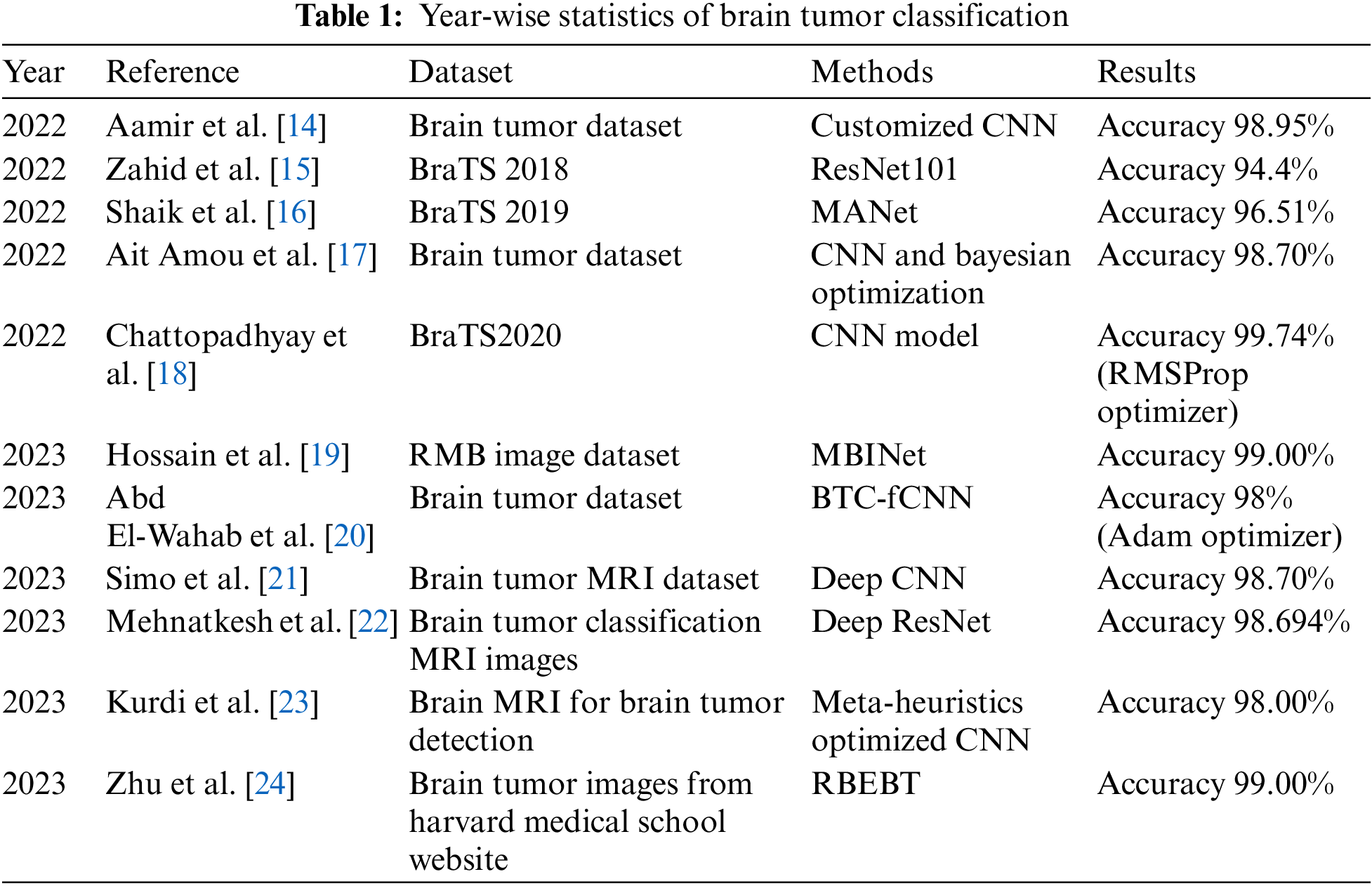
We have taken the recent work on brain tumor classification from 2022 and 2023. In all research works, CNN models are used for classification. We proposed a novel lightweight CNN model and trained it using the gradient-boosting algorithm to ensure higher accuracy.
We utilized our GliomaCNN for the classification task. For the dataset, BraTS 2020 [25–27] is used. Fig. 1 elucidates the intricacies of the proposed methodology.
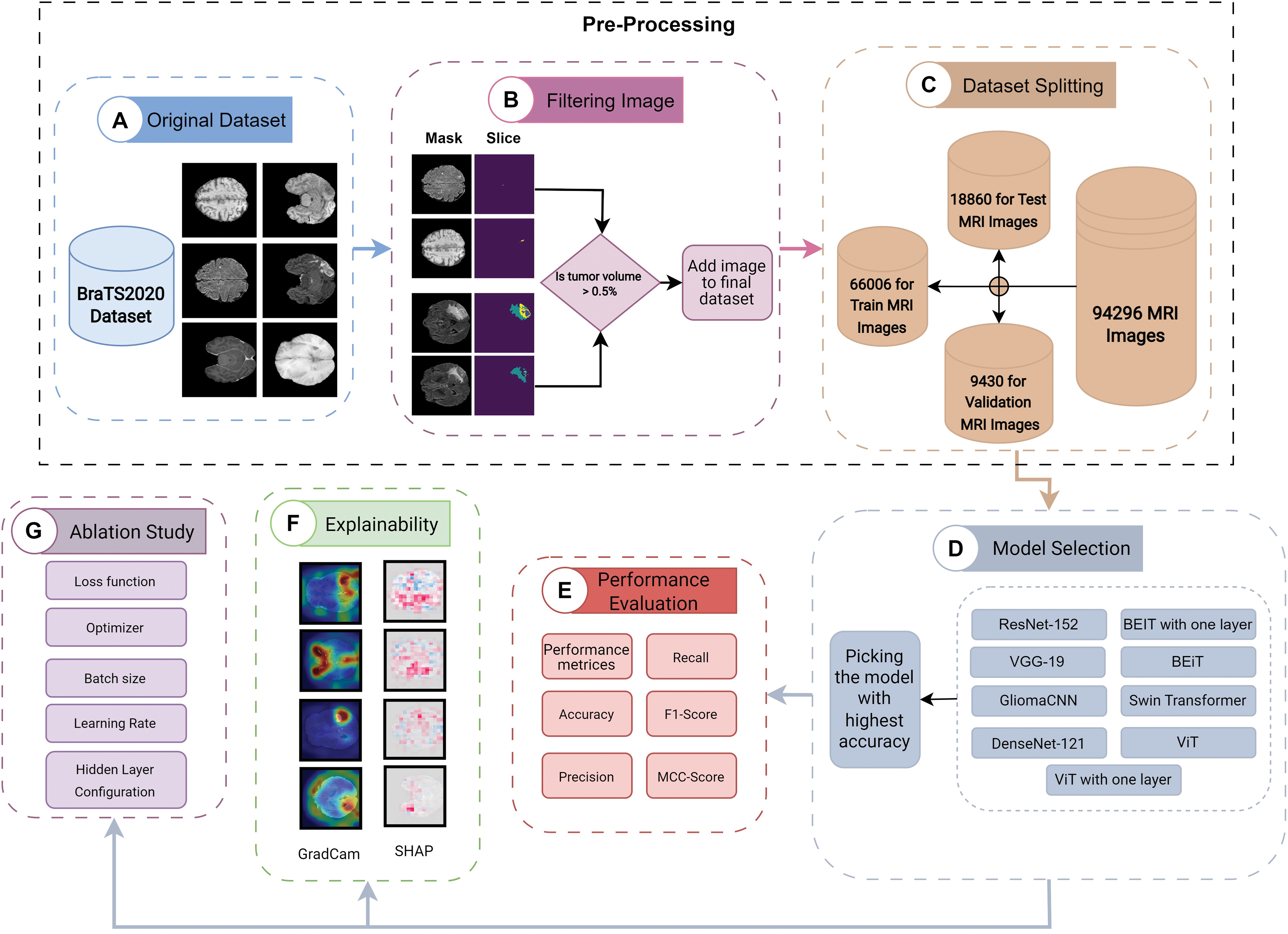
Figure 1: Proposed methodology
The proposed methodology is comprised of multiple steps:
1. The first crucial stage in the pre-processing process is the conversion of 3D images into 2D representations. The procedure then entails identifying and excluding images with less than 0.5% tumor annotation in the Region of Interest (ROI) mask. The dataset is finally divided into separate sets for training, validation, and testing.
2. Develop a lightweight CNN model with a few hidden layers.
3. Run multiple models and pick the model that gives the highest accuracy
4. Analysis of model performance using various performance metrics.
5. Impose explainable AI (XAI) to find the model interpretability.
6. An ablation study to determine the best combination of hyperparameters of the proposed model.
Many methods have been proposed for categorizing images. CNNs are a specific type of neural network that has proven highly effective in tasks like recognizing and classifying images.
Within the domain of computer vision, Convolutional Neural Networks have become dominant due to their exceptional accuracy in image classification. Convolution layers in these networks include the convolution, batch normalization, and max-pooling layer. When we think about an image, we can visualize it as a cuboid with channels, height, and width, as depicted in Fig. 2. For instance, a colored RGB image has three channels, while a grayscale image has just one. Fig. 3 depicts the convolution operation.
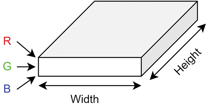
Figure 2: Representation of RGB image
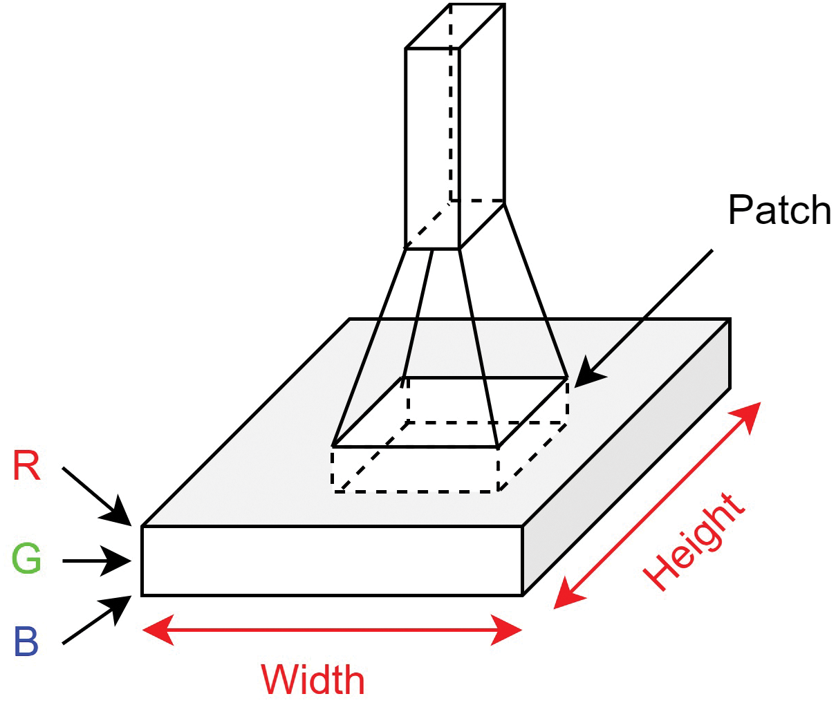
Figure 3: Convolution operation
To extract meaningful information from an image, we use a filter, also known as a kernel. Typically, this kernel is a smaller
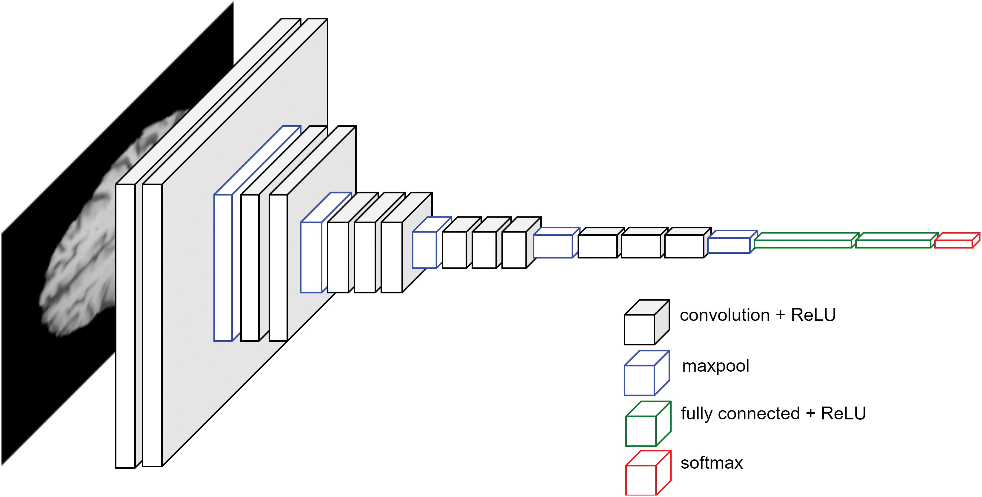
Figure 4: CNN architecture
The pooling layer is an essential component of CNNs. Its main role is to gradually shrink the spatial dimensions of the data, which helps in reducing the number of parameters and computational load in the network. This, in turn, helps prevent overfitting. The pooling layer works on each depth slice of the input separately and spatially resizes it. Different kinds of polling lanes are used, such as:
1. Max Pooling: It returns the highest value found in its immediate rectangular area.
2. Average Pooling: It returns the average value found in its immediate rectangular area.
3. Weighted Average Pooling: It returns the weighted average value found in its immediate rectangular area. The weight is based on distance from its center pixel.
4. Min Pooling: It returns the minimum value found in its immediate rectangular area.
Batch normalization (BN) is an algorithmic technique employed in the training of DNNs to enhance both the speed and stability of the learning process. Unlike operating on the entire dataset, BN operates within mini-batches of data. Its primary purpose is to expedite the training procedure, permitting the utilization of more substantial learning rates, thereby facilitating smoother and more efficient learning. Batch normalization formula can be defined as:
where
To classify an image, a fully connected layer after the convolution layers are added. Before passing the output of convolution layers, the output needs to be flattened. The final production of the fully connected layer is the logits. We propose a novel architecture GliomaCNN which is trained using the gradient-boosting [28] algorithm in which the base estimator is our GliomaCNN. Our CNN model is very small containing only three CNN layers each followed by a maxpool layer. The architecture of our GliomaCNN is given in Fig. 5.
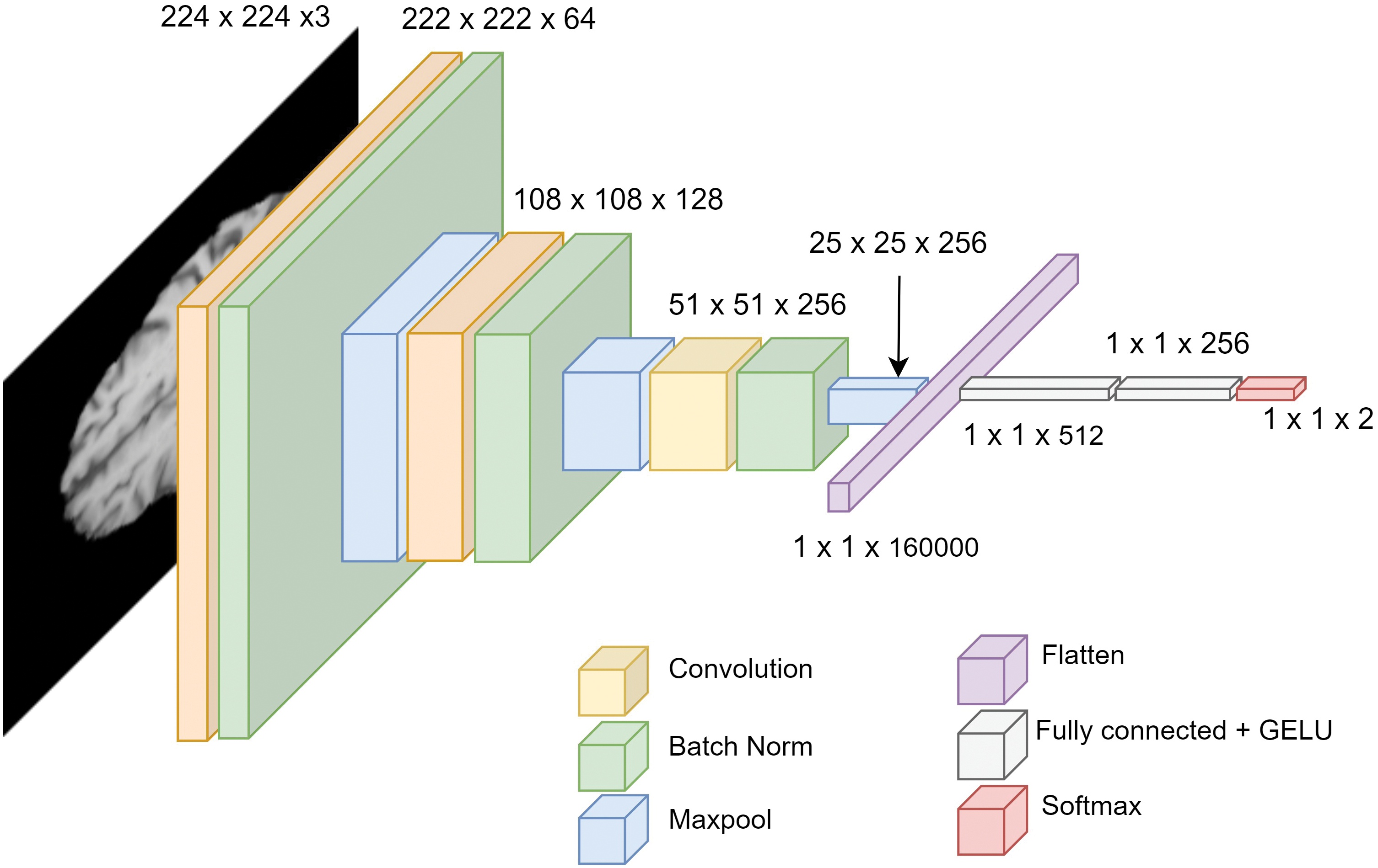
Figure 5: Architecture of GliomaCNN
All convolutional layers employ a kernel size of
There are 512 neurons in the first fully connected layer, 256 neurons in the second fully connected layer, and two neurons in the final layer as our dataset has two classes. For the activation function, the GELU [29] is used.
Fig. 6 depicts the parameters of each layer of the proposed CNN model. In convolution layer one, the Conv2D block has 1792 parameters. Batch normalization layer’s input is the output of the previous Conv2D block. The output of the first Conv2D block is 64 channels. So the input of BatchNorm2D is 64 channels. The parameter is double the input size because the mean and the standard deviation are calculated for each input channel of the BatchNorm2D layer. So, the total parameter of BatchNorm2D is 128. A similar calculation goes for convolution layer 2 and convolution layer 3. The total parameter from three convolution blocks is 371,712. The dense layer contains three linear layers. Only linear layers contribute to increasing the model’s parameters. The activation function does not have any parameters. The total parameter of the dense layer is
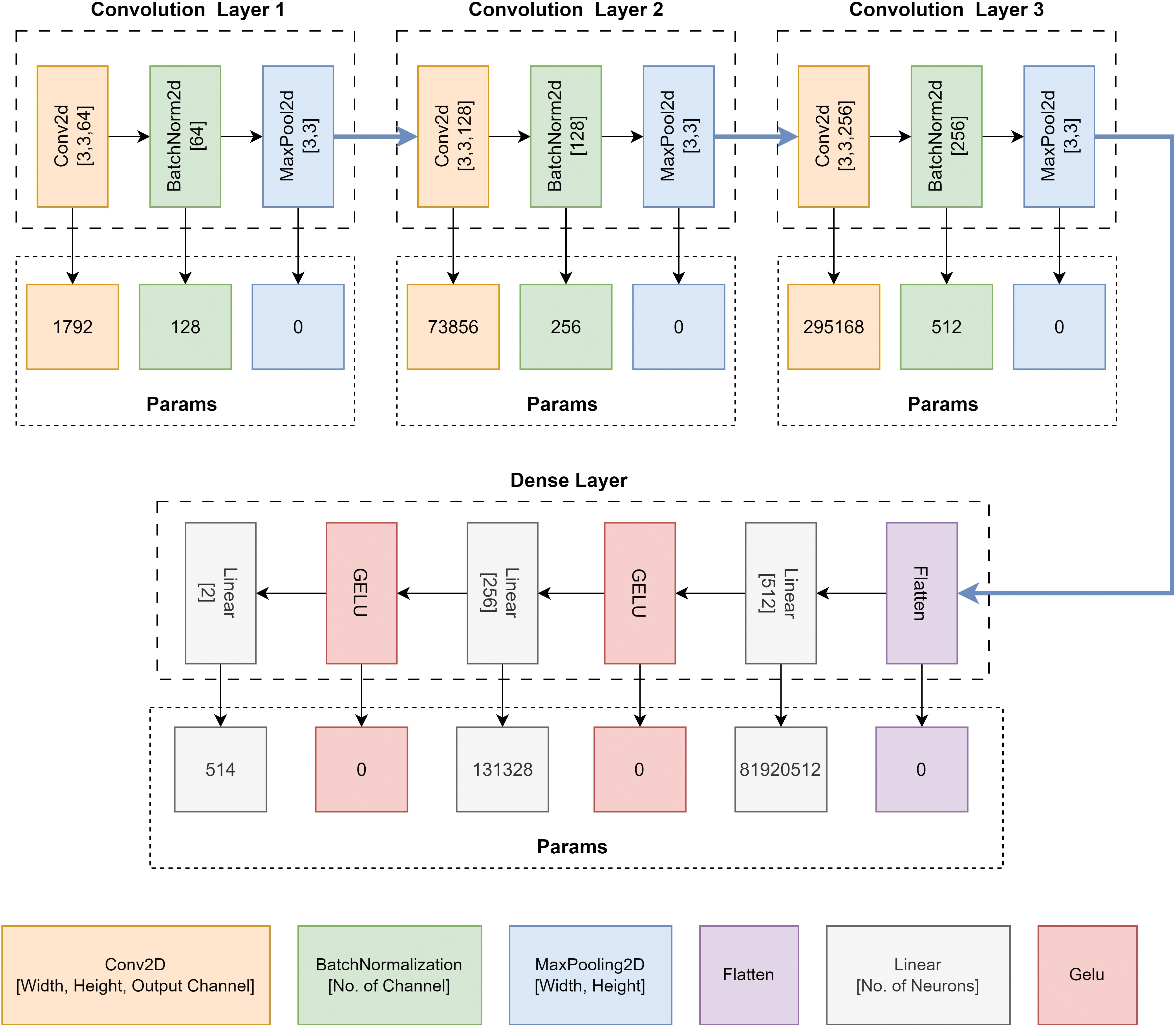
Figure 6: Parameter of the proposed CNN architecture, GliomaCNN
As previously mentioned, gradient boosting trains each base estimator sequentially. This is because the learning target
1. Decide the learning target on each sample
2. Fit the m-th base estimator using least square regression, that is,
3. Update the accumulated output:
Fig. 7 presents the data flow of gradient boosting during the training and evaluating stages, respectively. Notice that the training stage runs sequentially from the left to right.
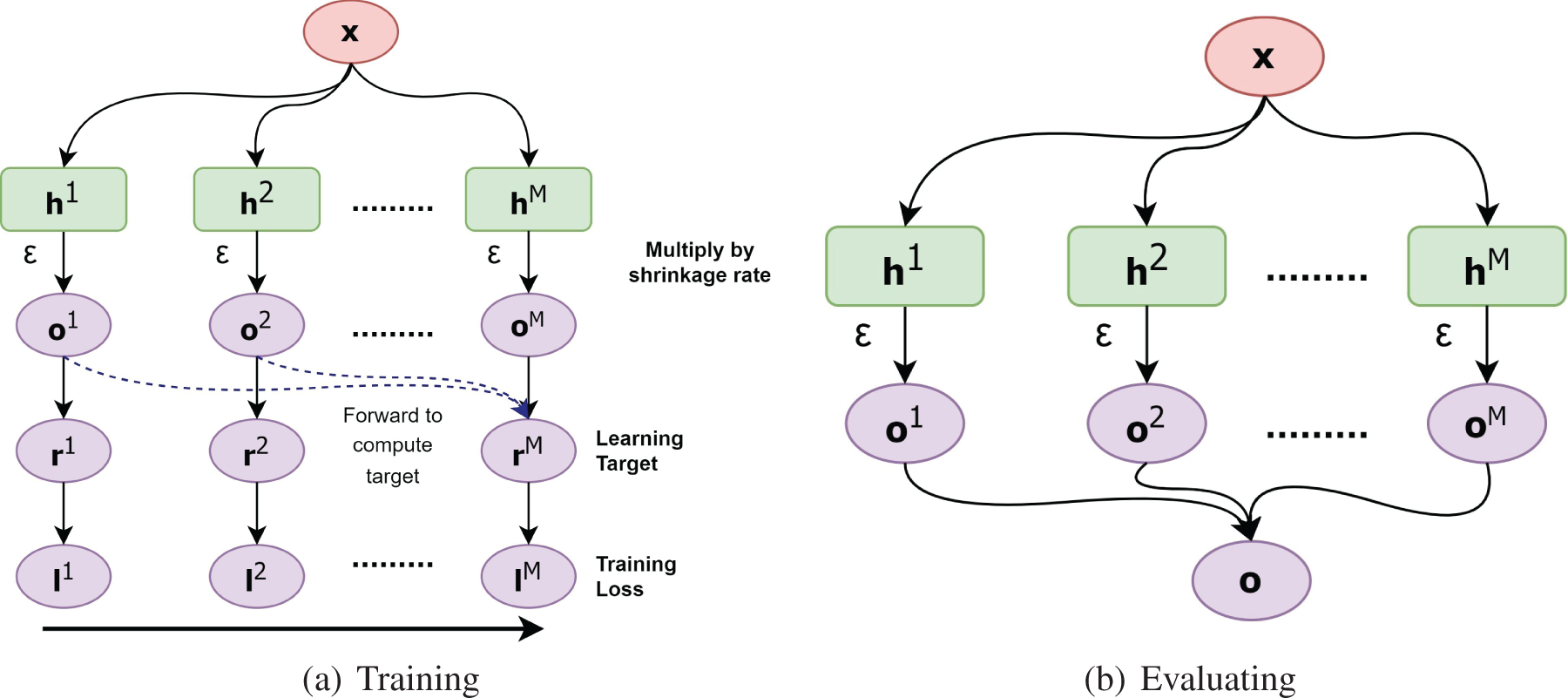
Figure 7: (a) refers the data flow during training and (b) shows the data flow during evaluation of gradient boosting algorithm
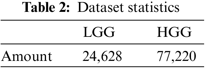
We used BraTS 2020 [25,26] for our research. This dataset has two classes: LGG and HGG. Two random MRI scans from the dataset are shown in Fig. 8. For a single patient, each dataset includes one ROI and four 3D MRI sequences (T1, T1-weighted, T2-weighted, and T2 Fluid Attenuated Inversion Recovery), all stored in Neuroimaging Informatics Technology Initiative (NIfTI) files. Each 3D volume also includes 150 2D MRI slices or images from various brain regions. The single slices are in single-channel grayscale format with a dimension of
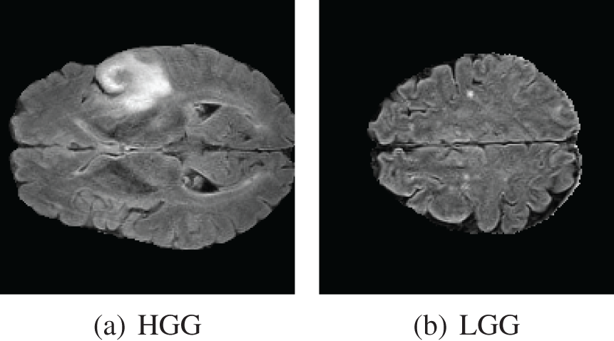
Figure 8: BraTS dataset contains two classes. (a) HGG and (b) LGG
As we are working with two-dimensional images, it is essential to use 2D image data exclusively. We obtained the dataset from Kaggle, comprising 57,198 Hierarchical Data Format-5 (HDF5) files containing 2D images that had been preprocessed from MRI sequences. Each HDF5 file contains four distinct MRI sequences. Following this, we conducted image cropping along all margins to eliminate the non-informative black regions surrounding the brain MRI scans. This strategic cropping procedure was employed to eliminate extraneous areas and optimize the precision of our classification outcomes. After cropping the images, the dimension of the new images became

Figure 9: Samples from the dataset
We implemented an additional filtering step utilizing the ROI images. In certain slices, the tumor occupies such a minimal portion that it becomes challenging to discern any abnormalities in the brain scan. To address this concern, we selected images where the mask contained a minimum of 0.5% annotation. Fig. 10 shows a brain scan from the HGG class with an ROI mask. The ROI mask features a yellow dot enclosed by a red outline, making it unidentifiable in the original brain scan. In this particular scan, there is no tumor present in the original brain scan but it is visible through the ROI mask. So it is quite impossible to detect this abnormality in the brain scan through visual inspection.
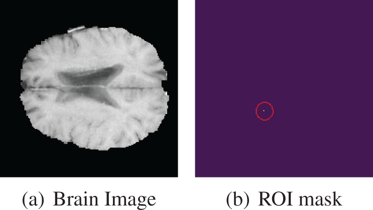
Figure 10: HGG brain scan with very small ROI mask
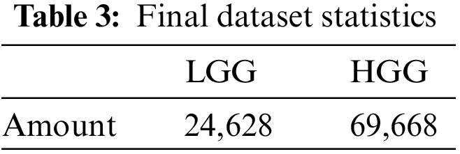
After filtering out the images by the above criteria, the total image count in our final dataset is shown in Table 3.
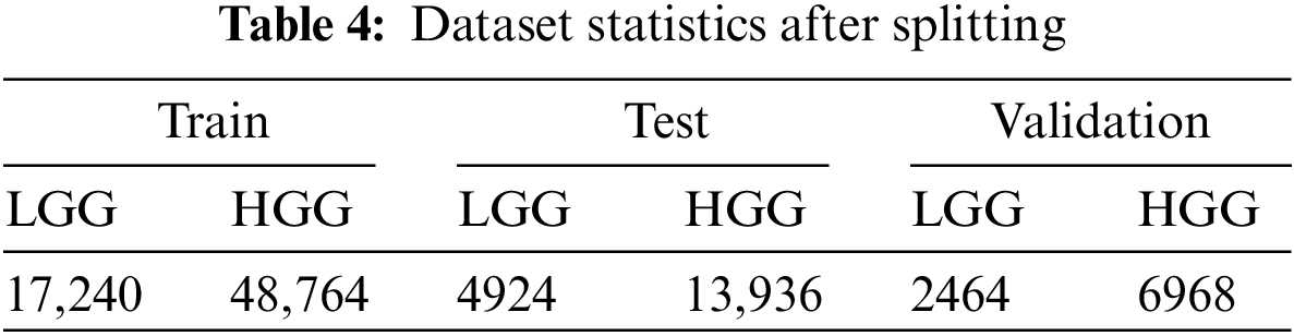
We partitioned the dataset using a 70:10:20 ratio into subsets for training, validation, and testing. During the data splitting process, we took great care to ensure that all MRI scans belonging to the same individual were correctly allocated to their respective sets. The amount of data after splitting is given Table 4.
In this research, We used the accuracy, recall, precision, F1-score, roc-auc score, and Mathews correlation coefficient to rate the performance of the models.
The accuracy or error rate is one of the most commonly utilized measures in practice by numerous researchers to assess classifier classification efficiency. The Eq. (2) represents the formula of accuracy:
Precision is the percentage of correct modules among those predicted to be defective. Precision is essential, especially when class distributions are heavily skewed. Using the Eq. (3) precision can be computed:
Recall counts the percentage of correct positive forecasts among all potential positive forecasts. The Eq. (4) is used to calculate the recall.
The harmonic mean of recall and precision is the F1-score. By dividing the precision and recall product by the sum of precision and recall, it can be calculated. The F1-score is obtained using Eq. (5).
3.4.5 Mathews Correlation Coefficient (MCC)
The Matthews correlation coefficient is used in machine learning to assess the precision of binary and multiclass classifications. It is considered a fair measure that may be applied even when the classes have sizes that are significantly different and take into account genuine and false positives and negatives. A correlation coefficient value between −1 and +1 is essentially what the MCC is. Average random prediction is indicated by a value of 0, whereas inverse prediction is indicated by a value of −1, and perfect prediction is indicated by a value of 1. Additionally, the statistic is known as the phi coefficient. The equation of the MCC score is 6:
Ablation studies investigate the performance of AI models by removing certain components to understand their performance. On a CNN model, an ablation study can be done by changing different models’ parameters and hyperparameters. For instance, a number of convolution layers, maxpool layers, kernel size, dense layers optimizer, and learning rate.
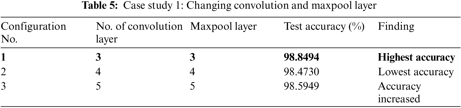
In case study 1, we varied the number of convolution layers. We increased the convolution layer count from three to five at first. The performance of the proposed model with various numbers of convolution layers is illustrated in Table 5. Configuration 1 gives the highest accuracy. The accuracy decreased when a second convolution layer with twice as many output channels as the first layer was added. Adding another convolution layer helped to increase the accuracy a little bit but it increased the model parameters.
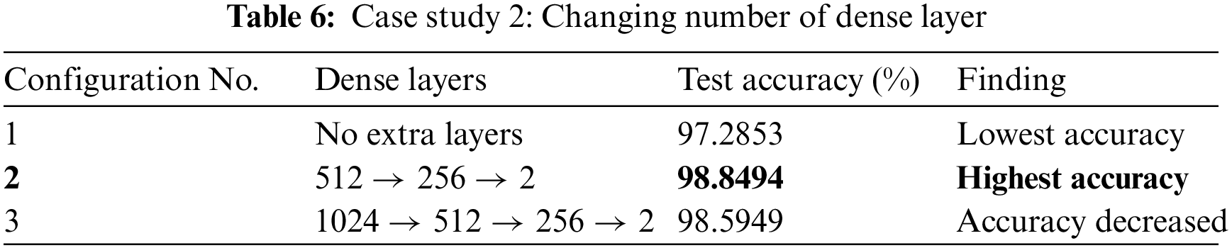
In our case study 2, we experimented with changing the number of dense layers in our model. The performance outcomes are detailed in Table 6. In Configuration 1, we maintained the baseline model without any additional dense layers. This led to a decrease in model accuracy. Configuration 2 achieved the highest accuracy. It incorporated three additional dense layers with 512, 256, and 2 nodes, respectively. Configuration 3 added one more dense layer with 1024 nodes, making a total of four dense layers. Though it did not fall below the accuracy of Configuration 1, it still didn’t quite match the performance achieved in Configuration 2.
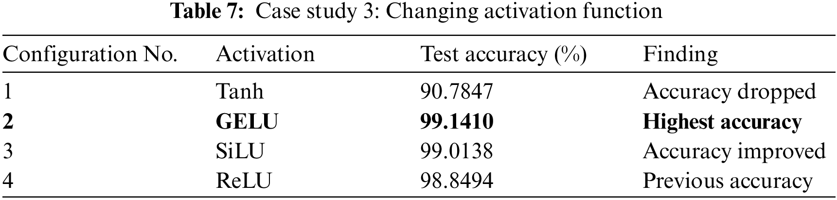
We tested the best-performer model from the previous two case studies with different activation functions. From this case study, We discovered that the performance of the model is significantly influenced by the activation functions. Table 7 presents the model’s accuracy when various activation functions are used. The GELU activation function gave us the highest accuracy whereas Tanh pulled down the accuracy to the worst. A little improvement was noticed when we changed the activation function from the Rectified Linear Unit (ReLU) to Sigmoid Linear Units (SiLU).
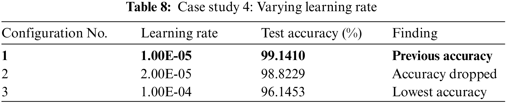
We tested with various learning rates on GliomaCNN in this case study. The outcomes are presented in Table 8. In Configuration 1, the model’s performance was evaluated with a learning rate of
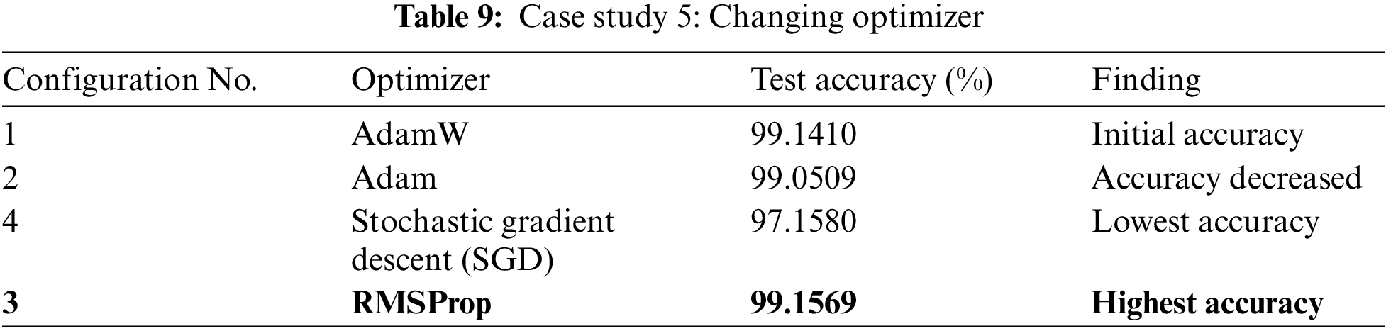
In case study 5, we tested GliomaCNN with different optimizers. Among all the optimizers we tested, RMSProp gave the highest accuracy of 99.1569%. AdamW gave the second-best outcome. The difference between the accuracies of using AdamW and RMSProp are very close. The SGD optimizer made the model performance worse. Table 9 shows the accuracy for each optimizer.
Our initial model architecture featured four convolutional layers, achieving an accuracy of 98.473%. Subsequently, we removed the last convolutional layer, leaving us with three convolutional and max-pooling layers, which led to an improved accuracy of 98.8498%. Throughout both configurations, we applied the ReLU activation function within the dense layers. Notably, switching from ReLU to the GELU activation function resulted in a modest accuracy boost, reaching 99.141%.
In the final stage of experimentation, we transitioned from the RMSProp optimizer, which was previously AdamW, and observed the highest achieved accuracy of 99.1569%.
Fig. 11 shows a bar chart illustrating the increase in accuracy by changing the model configuration.
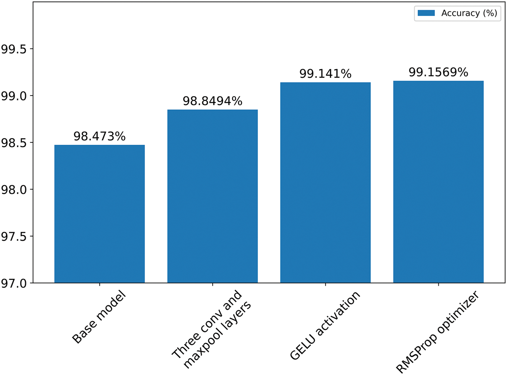
Figure 11: Summary of ablation study
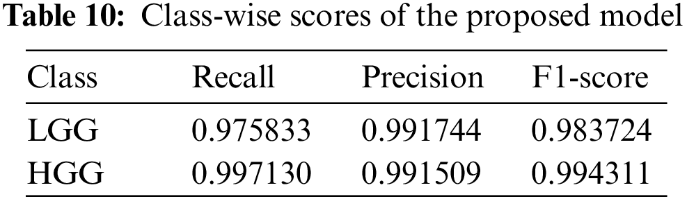
We achieve an accuracy of 99.1569% by doing the ablation study. The Table 10 presents the recall, precision, and F1-score of the individual classes of the GliomaCNN. The MCC score is 0.978. The scores imply that, even though the dataset is imbalanced, the model performs very well in classifying LGG and LGG brain images.
The confusion matrix in Fig. 12 illustrates the performance of the proposed model by displaying the count of images classified into each category. Label 0 represents class LGG, and label 1 represents class HGG. The misclassification rate of class LGG is higher, as can be seen from the confusion matrix. The dataset we used is imbalanced. This imbalance affected the performance of the model. The amount of images from the LGG class was much lower than that from the HGG class. Because of the lack of enough LGG class images, the GliomaCNN did not learn as well as the HGG class. That is why the misclassification rate is higher for the LGG class.
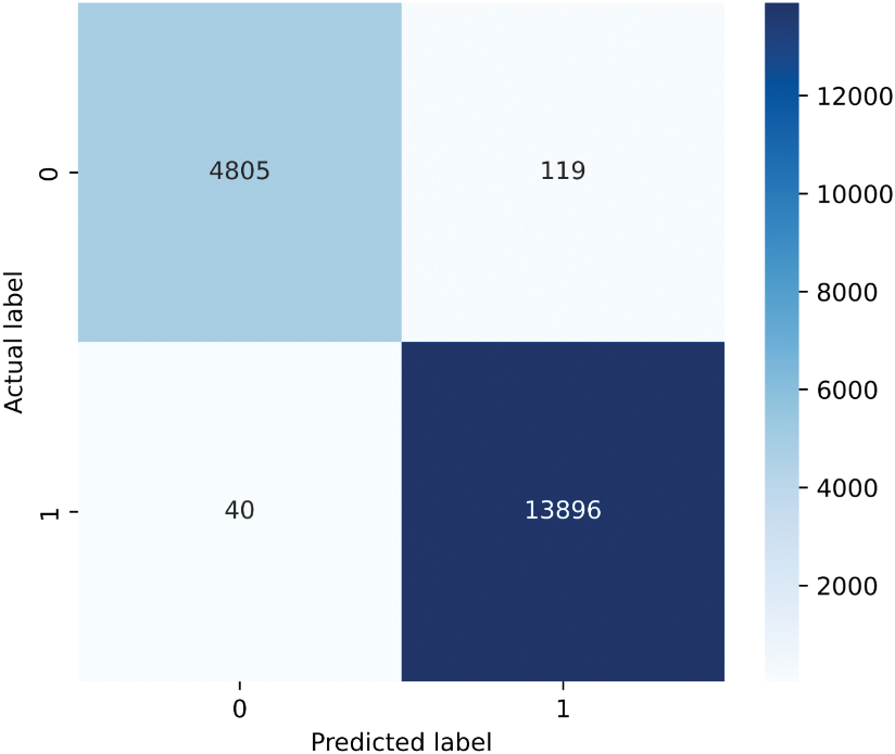
Figure 12: Confusion matrix
We have employed five sequential estimators in the gradient boosting algorithm, which is our proposed CNN model. Fig. 13 illustrates the training loss per epoch for each estimator, with the X-axis indicating the number of epochs and the Y-axis representing the percentage of loss and.
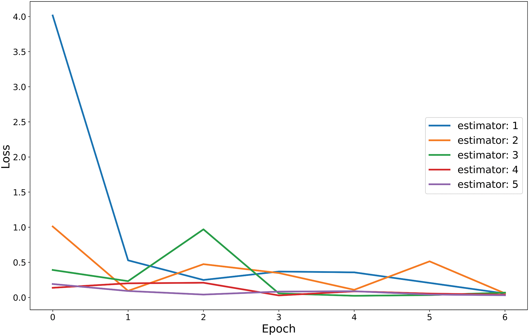
Figure 13: Train loss vs. epoch curve for five base estimators
Using the same dataset, we tested other pre-trained models and compared their results with our suggested model. Our model beats all other models. The Table 11 shows hyper-parameters, the test and validation results of all the tested models.
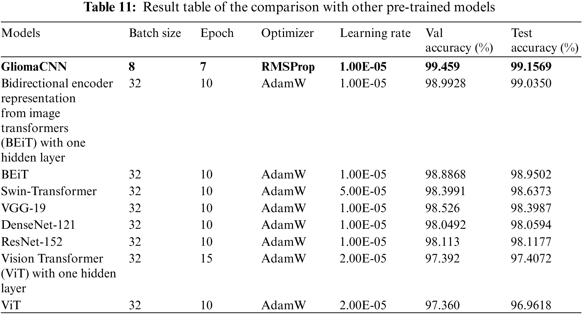
Fig. 14 illustrates a performance comparison between the proposed model and various pre-trained models. From the illustration, we can see our model outperforms the others in general, with the impact of data imbalance apparent in the bar charts. Notably, we achieve higher precision, recall, and F1-score for the HGG class compared to the LGG class, indicating our model’s effectiveness in distinguishing between them. The bar chart for accuracy and MCC score further emphasizes the exceptional performance of our model, GLiomaCNN, surpassing all other models in the comparison.
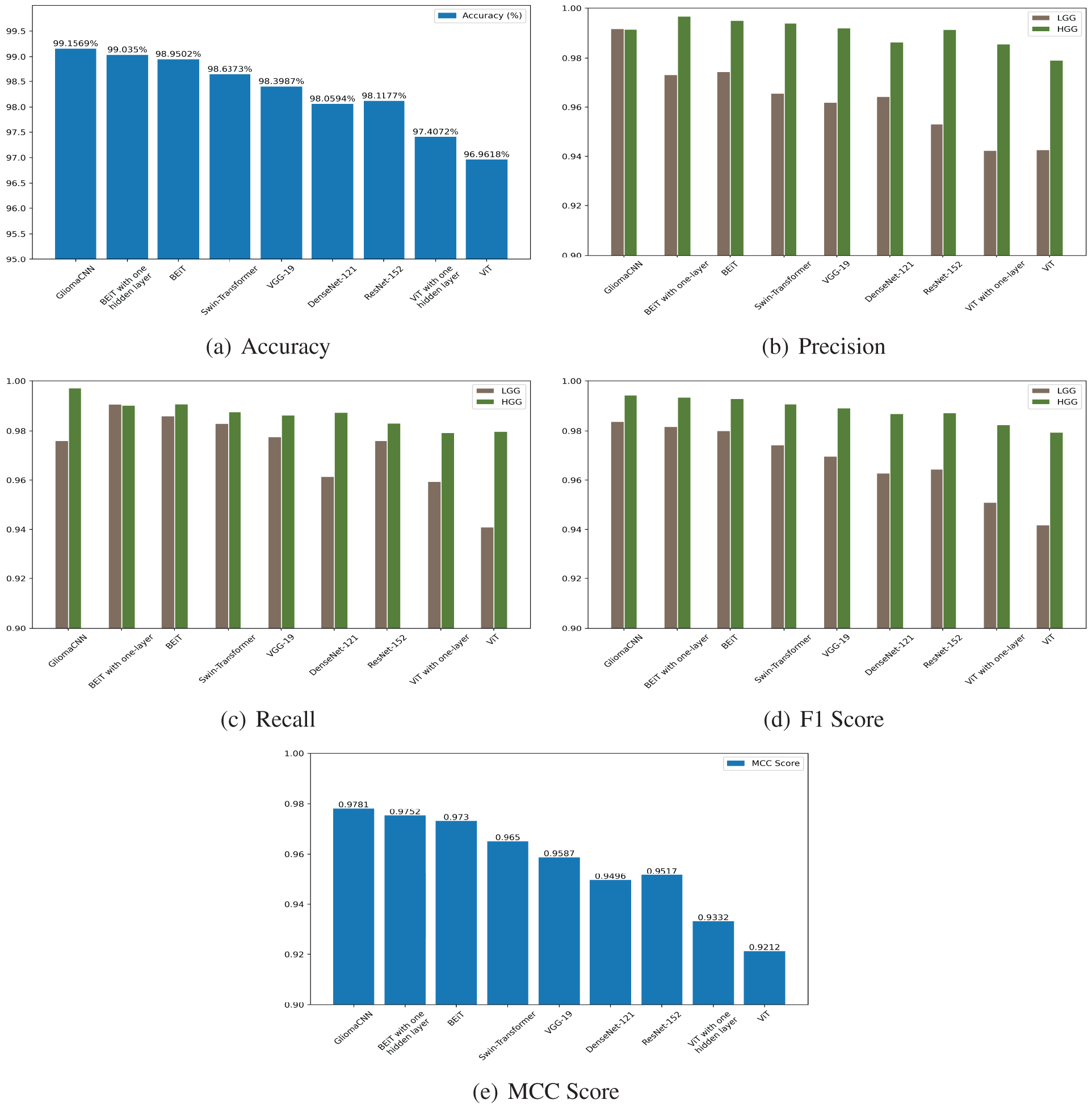
Figure 14: Test scores of all the tested models
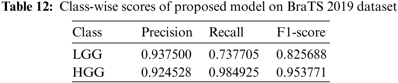
Using the BraTS 2019 dataset, we evaluated the performance of our model and obtained an accuracy of 92.6923%. Table 12 displays the class-wise results.
We compared our model’s performance against existing literature in the field of 2D MRI-based brain tumor analysis. Our evaluation is presented in Table 13. Table 13 shows that most results from prior studies fall within the range of 84% to 97% accuracy.
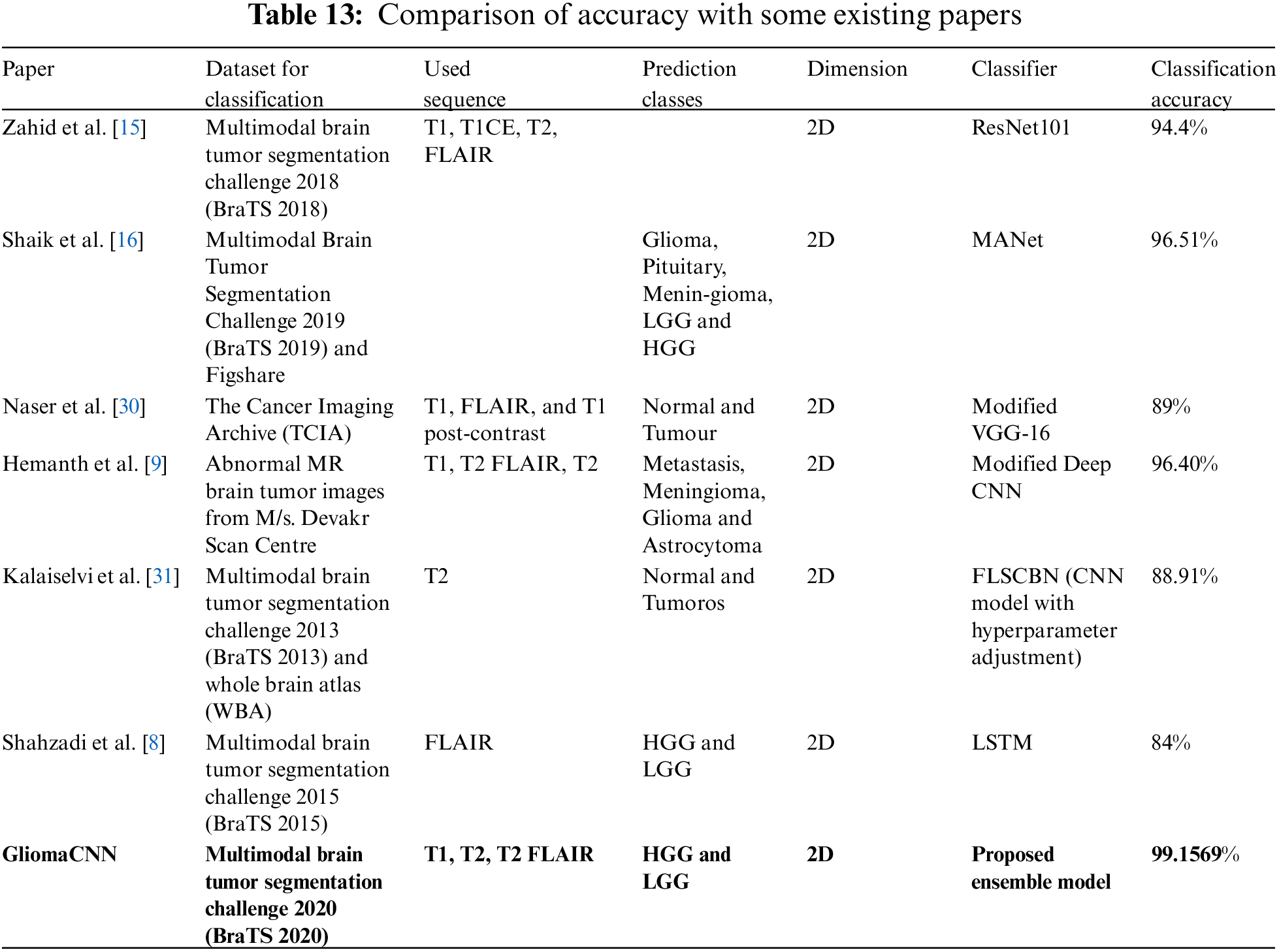
3.7 Comparison of Accuracy with Some Existing Papers
However, our model achieved a significantly higher accuracy of 99.1569%, as mentioned earlier. The highest accuracy among the referenced papers was recorded by Shaik et al. [16]. They have used a MANet to achieve an accuracy of 96.51%. The second highest accuracy among the referenced papers was recorded by Hemanth et al. [9]. They have used a modified Deep CNN classifier to obtain an accuracy of 96.40%. Zahid et al. [15] achieved 94.4% using ResNet101. Naser et al. [30] with a modified VGG-16 classifier used T1 pre-contrast, Fluid-attenuated inversion recovery (FLAIR), and T1 post-contrast 2D sequences, achieving 89% accuracy. Kalaiselvi et al. [31] reported an accuracy of 88.91% using T2 sequences on the BraTS 2013 dataset. In a similar vein to our work, Shahzadi et al. [8] employed LSTM for classifying HGG and LGG tumors. They achieved 84% accuracy on the BraTS 2015 dataset.
To understand how the model predicts and which regions are important for a particular prediction, explainable AI is employed. In this section, we analyze our proposed model’s prediction with two commonly used XAI frameworks which are SHAP and Grad-CAM++.
As AI technology advances, it becomes increasingly challenging for humans to comprehend and follow the inner workings of the algorithms involved. These algorithms often appear as enigmatic “black boxes,” with their intricate mathematical processes reduced to an unintelligible state. This opacity extends to the data-driven models they produce, rendering them inscrutable to even the engineers and data scientists responsible for their development. The ability to articulate precisely what transpires within these AI algorithms, let alone how they arrive at specific conclusions, often eludes those intimately familiar with their construction. Several research initiatives have been launched to improve the deep learning systems’ usability and transparency in response to this problem.
Using the game theoretically ideal Shapley values, Lundberg et al. [32] developed SHAP, a technique to explain specific predictions. This method aims to clarify predictions by assessing the role of each attribute. It makes use of a heatmap to visualize a proposed network and identify the target class by highlighting the critical image region. Blue areas signify a strong association with negative categorization, whereas pink regions indicate a pronounced link to positive classification. In essence, it reveals the areas of the image that the model values most highly for prediction purposes. The SHAP output on correctly classified MRI scan images is shown in Fig. 15.
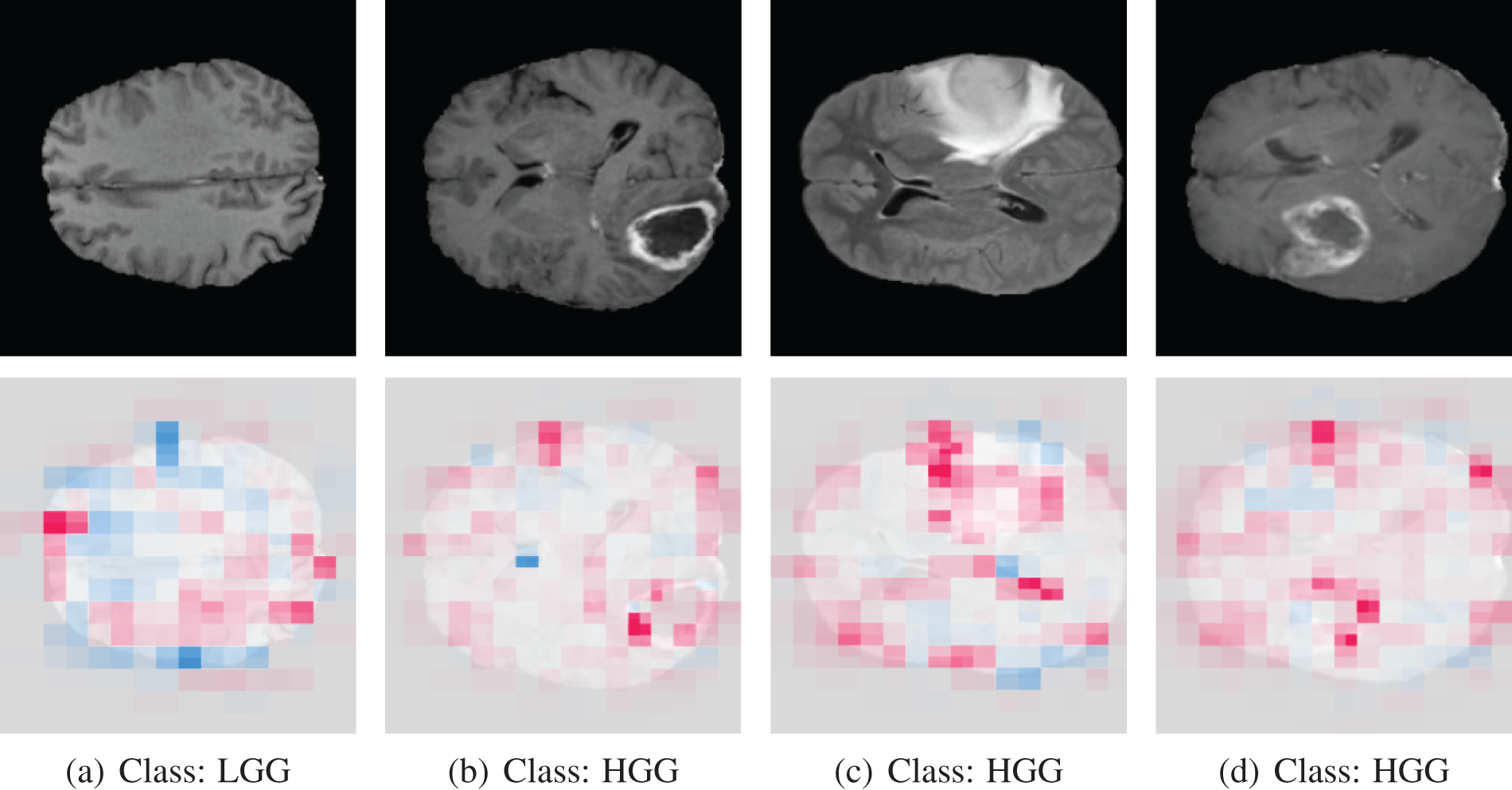
Figure 15: SHAP output of correctly classified images
The last three images belong to the HGG class, where the tumor is easily discernible. Examining the shape output, we notice that in the case of these last three images (b, c, d), the pink mark is prominently concentrated on the tumor region of the original image. Conversely, the first image belongs to the LGG class, where the tumor is not evident. In this instance, the SHAP markings are distributed across the entire image. By analyzing the heatmap image, we can deduce that our proposed model categorizes images based on the region that genuinely influences the determination of the tumor type.
The SHAP output on misclassified MRI scan images is shown in Fig. 16.
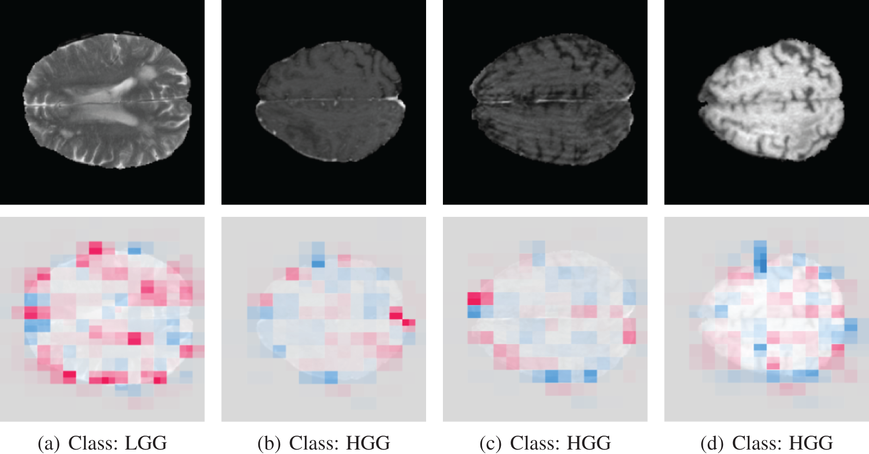
Figure 16: SHAP output of misclassified images. The model predicted the opposite of the actual class label
The model initially misclassified the first image as HGG when it was an LGG due to its confusion of normal brain tissue with a tumor, as revealed by SHAP analysis. Conversely, for other brain tumor images (b, c, d), the model incorrectly labeled them as LGG when they were HGG because it had difficulty pinpointing the precise tumor location, evident from the widespread pink marker in the SHAP analysis. GliomaCNN struggles to detect these tumors as they are not visible signs of tumors.
In a study by Selvaraju et al. [33], Grad-CAM was introduced as a technique to generate ‘visual explanations’ for decisions made by various CNN-based models, enhancing their interpretability. Grad-CAM enables visual evaluation of the model’s focus, ensuring it identifies relevant patterns in the image and activates accordingly.
From the CAM output of correctly classified images, the red-highlighting image regions are considered to be important for model prediction. The highlighted portion of the tumor indicates that our model can identify the tumor. From the CAM output of correctly classified images, the red-highlighting image regions are considered to be important for model prediction. The highlighted portion of the tumor indicates that our model can identify the tumor. The correctly classified original and Grad-CAM heatmap images are depicted in Fig. 17. In the first image, the tumor is not visible, and Grad-CAM++ highlighted the rightmost small portion of the image, which is the background. There is no visible tumor in that scan, so Grad-CAM++ did not highlight any portion of the brain, which makes sense.
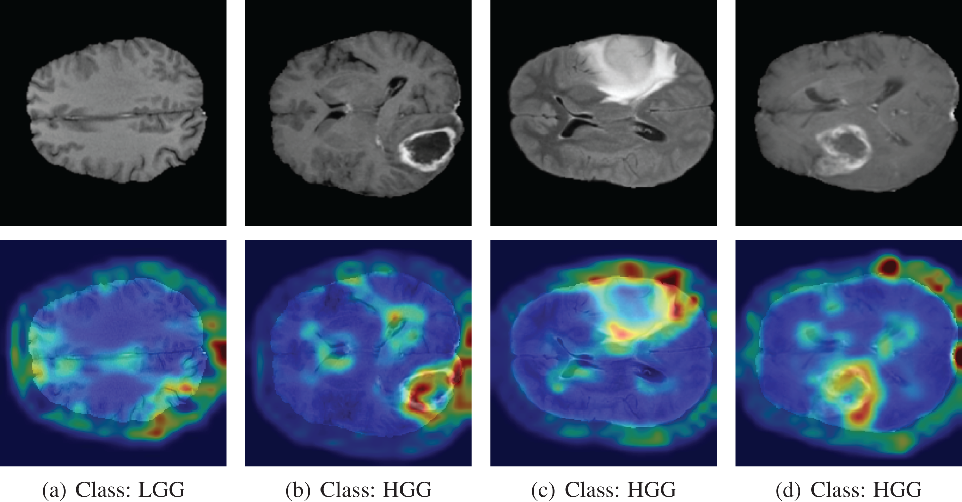
Figure 17: Grad-CAM output of correctly classified images
Analyzing the misclassified images, we found some interesting findings. The first image is from class LGG, but the model predicted it as HGG. The Grad-CAM++ heatmap shows the region of the brain where the color is whitish, like a tumor. However, it is not a tumor, though the marked region is similar to a tumor. The Grad-CAM++ output on misclassified MRI scan images is shown in Fig. 18.
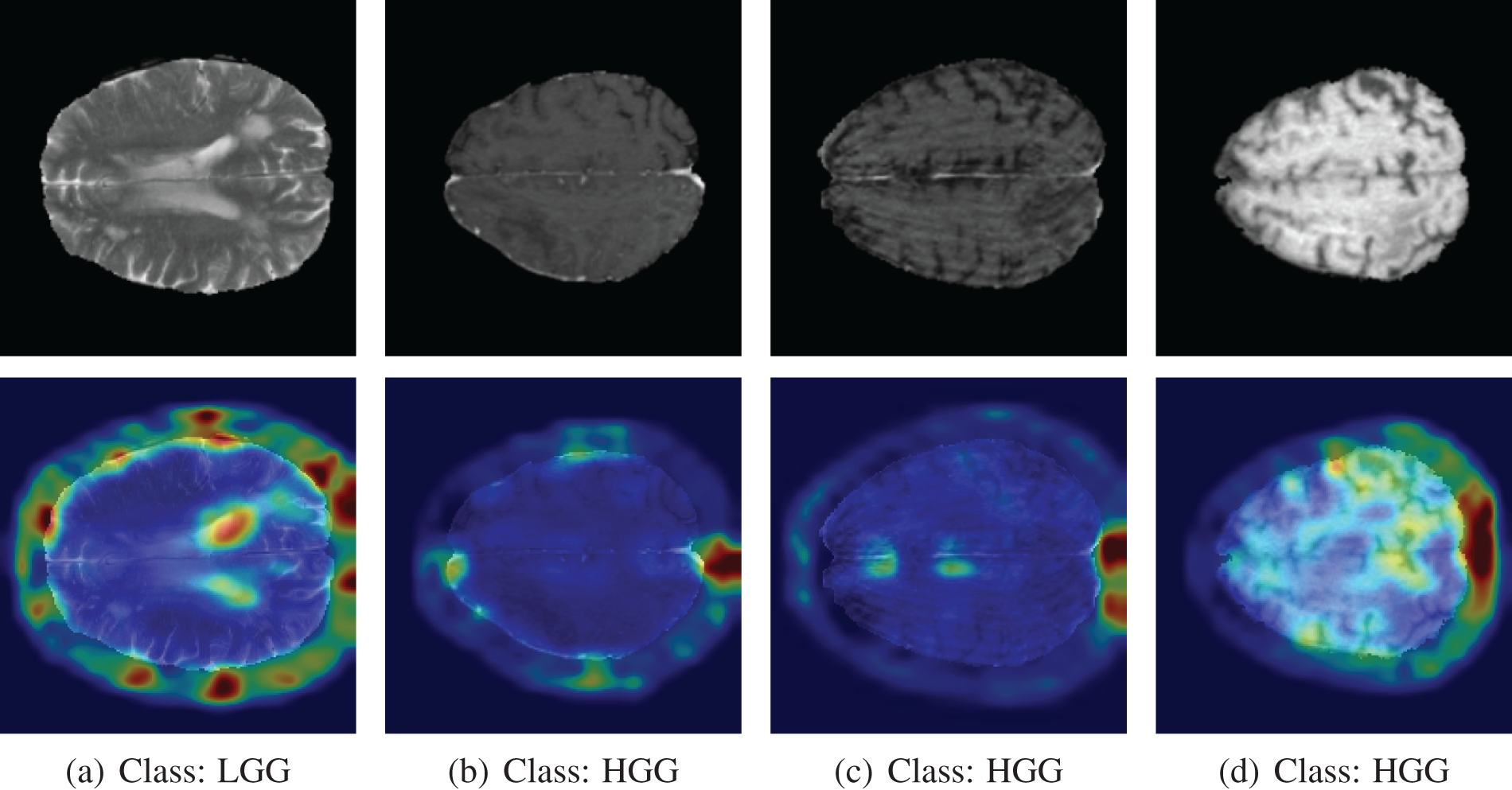
Figure 18: Grad-CAM++ output of misclassified images. The model predicted the opposite of the actual class label
For the other three images, the model predicted them as an LGG class. In those three scans, even though the images are from the HGG class, there is no visible sign of a tumor in the brain. The marking of Grad-CAM++ is random for those images. It is very hard to tell the presence of the tumor from the visual inspection of the last three images. The model misclassified those images because there is no solid sign of a tumor.
This study endeavors to propose an innovative lightweight CNN model called GliomaCNN, designed for the categorization of brain tumors into LGG and HGG, with an emphasis on achieving exceptionally high accuracy within the context of a highly imbalanced dataset. Our approach involves utilizing the proposed GliomaCNN as a base estimator for the gradient-boosting classifier. We achieved an outstanding accuracy of 99.1569%, which is remarkable for such a small CNN model. Our model performs best with the RMSProp optimizer in conjugation with 0.00001 learning rate. The validation accuracy was 99.459%. To understand the reasoning behind the classification, we used Grad-CAM++ and SHAP. These tools provide important insights by emphasizing the critical areas in the input photos that had a major impact on the model’s classification results. From the output of those two expandable AI methods, it can be concluded that our model classifies images based on the correct region. In several instances, these misclassifications stemmed from images where there were no discernible signs of a visible tumor. The model’s misclassification of such cases was found to be logically justified, as it is challenging for any classifier to correctly identify tumors in images where they are absent. Overall, we tried to develop a model as small as possible without compromising the performance. We succeeded in achieving a very high accuracy which beats all other state-of-the-art pre-trained models that we tested as well as other previous works in this field. In the future, We will test our GliomaCNN with other ensemble techniques, for instance, voting, snapshot ensemble, fast geometric ensemble, etc. We will employ more datasets not only brain tumor MRIs but also MRIs from other parts of the body. We plan to fine-tune the GliomaCNN model to extend its applicability for tumor classification in other anatomical regions.
Acknowledgement: The authors extend their appreciation to King Saud University for funding this research through Researchers Supporting Project Number (RSPD2024R1027), King Saud University, Riyadh, Saudi Arabia.
Funding Statement: This research is funded by the Researchers Supporting Project Number (RSPD2024R1027), King Saud University, Riyadh, Saudi Arabia.
Author Contributions: Conceptualization, M. -A. R., M. -I. M., K. -M. H.; methodology, data curation, M. - A. R., M. -I. M., K. -M. H., M. -F. M; software, M. -A. R., M. -I. M., M. S.; validation, M. -A. R., M. -I. M., K. -M. H., S. A., formal analysis, M. -A. R., M. -I. M., D. C.; investigation, M. -A. R., M. -I. M., M. S., S. A.; resources, M. -A. R.; writing-original draft preparation, M. -A. R., M. -I. M., K. -M. H.; writing-review and editing, M. -F. M, M. S., S. A., D. C.; visualization M. S.; project administration, M. -F. M., S. A.; supervision, M. -F. M., M. S. All authors have read and agreed to the published version of the manuscript.
Availability of Data and Materials: The data that support the findings of this study are available from the corresponding authors upon reasonable request. The datasets can be found here BraTS 2020, BraTS 2019.
Conflicts of Interest: The authors declare no conflict of interest to report regarding the present study.
References
1. Ferlay J, Soerjomataram I, Dikshit R, Eser S, Mathers C, Rebelo M, et al. Cancer incidence and mortality worldwide: sources, methods and major patterns in GLOBOCAN 2012. Int J Cancer. 2015;136(5):E359–86. doi:10.1002/ijc.29210. [Google Scholar] [PubMed] [CrossRef]
2. Chatterjee S, Nizamani FA, Nürnberger A, Speck O. Classification of brain tumours in MR images using deep spatiospatial models. Sci Rep. 2022;12(1):1505. doi:10.1038/s41598-022-05572-6. [Google Scholar] [PubMed] [CrossRef]
3. Teng C, Zhu Y, Li Y, Dai L, Pan Z, Wanggou S, et al. Recurrence-and malignant progression-associated biomarkers in low-grade gliomas and their roles in immunotherapy. Front Immunol. 2022;13:899710. doi:10.3389/fimmu.2022.899710. [Google Scholar] [PubMed] [CrossRef]
4. David DS, Saravanan D, Jayachandran A. Deep convolutional neural network based early diagnosis of multi class brain tumour classification system. Solid State Technol. 2020;63(6):3599–623. [Google Scholar]
5. Szwarc P, Kawa J, Rudzki M, Pietka E. Automatic brain tumour detection and neovasculature assessment with multiseries MRI analysis. Comput Med Imaging Graph. 2015;46(1):178–90. doi:10.1016/j.compmedimag.2015.06.002. [Google Scholar] [PubMed] [CrossRef]
6. Baranwal SK, Jaiswal K, Vaibhav K, Kumar A, Srikantaswamy R. Performance analysis of brain tumour image classification using CNN and SVM. In: 2020 Second International Conference on Inventive Research in Computing Applications (ICIRCA); 2020; Coimbatore, India, IEEE. p. 537–42. [Google Scholar]
7. Rasool M, Ismail NA, Boulila W, Ammar A, Samma H, Yafooz WM, et al. A hybrid deep learning model for brain tumour classification. Entropy. 2022;24(6):799. [Google Scholar] [PubMed]
8. Shahzadi I, Tang TB, Meriadeau F, Quyyum A. CNN-LSTM: cascaded framework for brain tumour classification. In: 2018 IEEE-EMBS Conference on Biomedical Engineering and Sciences (IECBES); 2018; Sarawak, Malaysia IEEE. p. 633–7. [Google Scholar]
9. Hemanth DJ, Anitha J, Naaji A, Geman O, Popescu DE, Hoang Son L. A modified deep convolutional neural network for abnormal brain image classification. IEEE Access. 2019;7:4275–83. [Google Scholar]
10. Montaha S, Azam S, Rafid ARH, Hasan MZ, Karim A, Islam A. Timedistributed-cnn-lstm: a hybrid approach combining CNN and LSTM to classify brain tumor on 3D MRI scans performing ablation study. IEEE Access. 2022;10:60039–59. [Google Scholar]
11. Ghnemat R, Alodibat S, Abu Al-Haija Q. Explainable artificial intelligence (XAI) for deep learning based medical imaging classification. J Imaging. 2023;9(9):177. [Google Scholar] [PubMed]
12. Zeineldin RA, Karar ME, Elshaer Z, Coburger J, Wirtz CR, Burgert O, et al. Explainability of deep neural networks for MRI analysis of brain tumors. Int J Comput Assist Radiol Surg. 2022;17(9):1673–83. [Google Scholar] [PubMed]
13. Gaur L, Bhandari M, Razdan T, Mallik S, Zhao Z. Explanation-driven deep learning model for prediction of brain tumour status using MRI image data. Front Genet. 2022;13:448. doi:10.3389/fgene.2022.822666. [Google Scholar] [PubMed] [CrossRef]
14. Aamir M, Rahman Z, Dayo ZA, Abro WA, Uddin MI, Khan I, et al. A deep learning approach for brain tumor classification using MRI images. Comput Elect Eng. 2022;101(5):108105. doi:10.1016/j.compeleceng.2022.108105. [Google Scholar] [CrossRef]
15. Zahid U, Ashraf I, Khan MA, Alhaisoni M, Yahya KM, Hussein HS, et al. BrainNet: optimal deep learning feature fusion for brain tumor classification. Comput Intell Neurosci. 2022;2022(2):1–13. doi:10.1155/2022/1465173. [Google Scholar] [PubMed] [CrossRef]
16. Shaik NS, Cherukuri TK. Multi-level attention network: application to brain tumor classification. Signal, Image Video Process. 2022;16(3):817–24. doi:10.1007/s11760-021-02022-0. [Google Scholar] [CrossRef]
17. Ait Amou M, Xia K, Kamhi S, Mouhafid M. A novel MRI diagnosis method for brain tumor classification based on CNN and bayesian optimization. Healthcare. 2022;10:494. [Google Scholar] [PubMed]
18. Chattopadhyay A, Maitra M. MRI-based brain tumour image detection using CNN based deep learning method. Neurosci Inform. 2022;2(4):100060. doi:10.1016/j.neuri.2022.100060. [Google Scholar] [CrossRef]
19. Hossain A, Islam MT, Abdul Rahim SK, Rahman MA, Rahman T, Arshad H, et al. A lightweight deep learning based microwave brain image network model for brain tumor classification using reconstructed microwave brain (RMB) images. Biosensors. 2023;13(2):238. doi:10.3390/bios13020238. [Google Scholar] [PubMed] [CrossRef]
20. Abd El-Wahab BS, Nasr ME, Khamis S, Ashour AS. Fast convolution neural network for multi-class brain tumor classification. Health Inf Sci Sys. 2023;11(1):3. doi:10.1007/s13755-022-00203-w. [Google Scholar] [PubMed] [CrossRef]
21. Simo AMD, Kouanou AT, Monthe V, Nana MK, Lonla BM. Introducing a deep learning method for brain tumor classification using MRI data towards better performance. Inform Med Unlocked. 2024;44(16):101423. doi:10.1016/j.imu.2023.101423. [Google Scholar] [CrossRef]
22. Mehnatkesh H, Jalali SMJ, Khosravi A, Nahavandi S. An intelligent driven deep residual learning framework for brain tumor classification using MRI images. Expert Syst Appl. 2023;213(7):119087. doi:10.1016/j.eswa.2022.119087. [Google Scholar] [CrossRef]
23. Kurdi SZ, Ali MH, Jaber MM, Saba T, Rehman A, Damaševičius R. Brain tumor classification using meta-heuristic optimized convolutional neural networks. J Pers Med. 2023;13(2):181. doi:10.3390/jpm13020181. [Google Scholar] [PubMed] [CrossRef]
24. Zhu Z, Khan MA, Wang SH, Zhang YD. RBEBT: a ResNet-Based BA-ELM for brain tumor classification. Comput Mater Contin. 2023;74(1):101–11. doi:10.32604/cmc.2023.030790. [Google Scholar] [CrossRef]
25. Menze BH, Jakab A, Bauer S, Kalpathy-Cramer J, Farahani K, Kirby J, et al. The multimodal brain tumor image segmentation benchmark (BRATS). IEEE Trans Med Imaging. 2014;34(10):1993–2024. [Google Scholar] [PubMed]
26. Bakas S, Akbari H, Sotiras A, Bilello M, Rozycki M, Kirby JS, et al. Advancing the cancer genome atlas glioma MRI collections with expert segmentation labels and radiomic features. Sci Data. 2017;4(1):1–13. [Google Scholar]
27. Bakas S, Reyes M, Jakab A, Bauer S, Rempfler M, Crimi A, et al. Identifying the best machine learning algorithms for brain tumor segmentation, progression assessment, and overall survival prediction in the BRATS challenge. arXiv preprint arXiv:181102629. 2018. [Google Scholar]
28. Friedman JH. Greedy function approximation: a gradient boosting machine. Ann Stat. 2001;29:1189–232. [Google Scholar]
29. Hendrycks D, Gimpel K. Gaussian error linear units (GELUs). arXiv preprint arXiv:160608415. 2016. [Google Scholar]
30. Naser MA, Deen MJ. Brain tumor segmentation and grading of lower-grade glioma using deep learning in MRI images. Comput Biol Med. 2020;121:103758. [Google Scholar] [PubMed]
31. Kalaiselvi T, Padmapriya T, Sriramakrishnan P, Priyadharshini V. Development of automatic glioma brain tumor detection system using deep convolutional neural networks. Int J Imaging Syst Technol. 2020;30(4):926–38. doi:10.1002/ima.22433. [Google Scholar] [CrossRef]
32. Lundberg SM, Lee SI. A unified approach to interpreting model predictions. Adv Neural Inf Process Syst. 2017;30. [Google Scholar]
33. Selvaraju RR, Cogswell M, Das A, Vedantam R, Parikh D, Batra D. Grad-CAM: visual explanations from deep networks via gradient-based localization. In: Proceedings of the IEEE International Conference on Computer Vision; 2017; Italy. p. 618–26. [Google Scholar]
Cite This Article
 Copyright © 2024 The Author(s). Published by Tech Science Press.
This work is licensed under a Creative Commons Attribution 4.0 International License , which permits unrestricted use, distribution, and reproduction in any medium, provided the original work is properly cited.
 Downloads
 Citation Tools