An Elastoplastic Fracture Model Based on Bond-Based Peridynamics

1  Introduction

Plastic deformation and failure are important problems in computational mechanics. When the ductile material is subjected to heavy loads, especially cyclic loads, it undergoes damage on the micro-scale along with plastic deformation. Once the damage develops, microcracks nucleate, propagate and coalesce to form macroscopic cracks. Numerous constitutive models have been proposed on the basis of continuum mechanics to describe the plastic deformation and failure behavior of materials. However, partial differential equations that compose continuum-based numerical approaches fail to describe the discontinuities in materials, such as cracks or voids, without involving additional techniques. As a consequence, elastoplastic models based on classical continuum mechanics have inherent limitations in solving problems concerning fracture.

To address fracture problems, some crack modeling methods have been proposed, among which are the cracking particle method [1] and the cracking elements method [2]. These methods can employ all types of constitutive models but easily allow modeling fracture. In 2000, Silling [3] introduced the peridynamic theory. As a nonlocal continuum theory, it replaces partial differential equations with integral equations, making it possible to solve fracture problems without any prior information. Compared with traditional methods, peridynamics has excellent fracture modeling capability [4], which is appealing in damage studies of various materials [5–9]. Apart from these applications, some nonlocal differential operators have been embedded in peridynamic theory, which includes the peridynamic differential operator [10], nonlocal operator method [11], and dual-horizon peridynamics [12]. These tools enable peridynamics to solve muti-physics and interface damage problems.

In the existing reports on plasticity problems based on peridynamic theory, the state-based peridynamic (SB-PD) model [13] is a commonly employed approach. In this model, the bond force is related to the displacements of all particles in the horizon, and the definition of the “state” allows for the convenient incorporation of classical constitutive models based on continuum mechanics. This enables the elastoplastic behavior to be addressed by introducing the appropriate constitutive model. Building upon the SB-PD model, extensive studies have been conducted on elastoplastic materials.

Madenci et al. [14] proposed the ordinary state-based PD plastic model using the von Mises yield criterion under isotropic hardening conditions. Liu et al. [15] have presented a general state-based peridynamic model, which can simulate perfect plastic, linear hardening and nonlinear hardening plastic behaviors. They also established an expression for the equivalent plastic stress in the non-local state-based peridynamic formulation. Zhou et al. [16] introduced a two-dimensional SB-PD model with plastic hardening deformation based on the Drucker-Prager criterion and the non-associated flow rule to analyze the plastic behavior of geotechnical materials. Mousavi et al. [17] offered an elastoplastic model considering the 2D plane stress/strain conditions based on the native ordinary state-based peridynamics. This advanced model has the capability to handle both small strains and large rotations. Zhang et al. [18] have proposed a unified elasto-viscoplastic peridynamic model by integrating Bodner-Partom’s constitutive theory into the ordinary state-based PD framework. This model allows describing the complete deformation-damage-fracture process for both brittle and ductile materials under impact loading conditions.

Based on the above works, significant progress has been made in addressing the issues relying on deformation, damage, and fracture of plastic materials [19–22]. However, the SB-PD model, with its complex control equations and strong numerical oscillations, poses challenges in ensuring computational stability. In contrast, the bond-based peridynamic (BB-PD) model simplifies the relationship between bond forces and relative displacements between adjacent material particles, resulting in a more streamlined strategy and higher computational efficiency. Therefore, successful plastic modeling using the BB-PD theory may overcome the shortcomings and limitations of the SB-PD approach, as well as increase the efficiency and robustness in applications involving elastoplastic behaviors of materials.

Since the conventional mechanical stress is not defined in the BB-PD model, it becomes difficult to describe plasticity directly using the classical plastic theory. To the best of our knowledge, there are a few studies on the BB-PD model to date. The pioneering work consisting of plastic analysis using BB-PD theory in conjunction with the microplastic constitutive model was divulged by Macek et al. [23] in 2007. In recent research, a generalized bond-based correspondence model has been proposed by Chen et al. [24] to simulate fracture. In this model, a specific function between peridynamic pairwise force and stress has been employed, making it possible to easily adopt plastic constitutive equations from continuum mechanics so as to predict the effect of plastic parameters on the dynamic fracture of quasi-brittle materials. However, Ladányi et al. [25] have pointed out that plastic deformation can be directly described through the bond force function without any additional transformation, thus enabling the extension of the peridynamic material model (PMM) to the isotropic hardening model. Meanwhile, the fracture of the material has not been taken into account.

In this work, an elastoplastic fracture model using the BB-PD theory is developed by considering the one-dimensional axial rod elastoplastic behavior of continuum mechanics. This model allows simulation of the plastic behavior of the material using both the linear and nonlinear-hardening laws, thus expanding the application scope of the bond-based peridynamics. Moreover, the bond damage is incorporated to model the fracture of the material. Compared with the existing peridynamics-based plastic models, the proposed version directly establishes the elastoplastic theory at the bond level without the need for additional calculation means. This endows the presented model with a concise form and higher computational efficiency compared to SB-PD plastic models.

The paper is organized into 6 sections. Section 1 is the introduction. Section 2 reviews and summarizes the BB-PD theory and its formulations. The elastoplastic model is presented and discussed in Section 3. Section 4 is devoted to the bond force updates and the numerical analysis based on the BB-PD model. In Section 5, five numerical examples are presented to verify the accuracy of the approach and demonstrate the capability and robustness of the model. Section 6 represents the conclusions with discussions and perspectives.

2  Brief Review of BB-PD Theory

In the bond-based peridynamic theory, the material is regarded as a set of particles in which each single particle interacts with other particles within a certain region, as shown in Fig. 1. The region is defined by a certain radius δ and is called horizon. The interaction between the particles is called “bond”, which contains all the constitutive information about the material.

Figure 1: Illustration of peridynamics discretization strategy

Assuming that there are two particles x and x′, the initial relative position vector between them is defined as

ξ=x′−x(1)

If the particles undergo the displacements u(x,t) and u(x′,t), respectively, at time t, then the relative displacement vector can be expressed as

η=u(x′,t)−u(x,t)(2)

The stretch of the bond is defined as

s=|η+ξ|−|ξ||η+ξ|(3)

According to Silling [1], the pairwise force vector f for a homogeneous objective microelastic material can be written as

f=cs(ξ,η)(4)

where c is the micromodule, which can be obtained from the equivalence of strain energy of a stretched truss in the classical and peridynamic models. Depending on the situation, the value of c can be found as [26]

c={6Eπhδ4(1−2ν)          (ν=14)three dimensional6Eπhδ3(1−ν)(ν=13)plane stress6Eπhδ3(1+ν)(1−2ν)(ν=14)plane strain(5)

Consequently, the equation of motion of a particle x with time t in the BB-PD can be written as

ρu¨(x,t)=∫Hxf(u(x′,t)−u(x,t),x′−x)dVx′+b(x,t)(6)

where u¨ refers to the acceleration of the particle x, ρ denotes the mass density, b represents the external force per unit reference volume, Hx is the horizon, and f corresponds to the force density vector on the particle x due to the impact of the particle x′ at time t.

3  Elastoplastic Fracture Model in Peridynamics

According to Ladányi et al. [24], the cumulative effect of numerous bond plastic deformations determines the plastic behavior at the macroscopic scale. Since the fracture of the ductile material is always accompanied by plastic deformation, plasticity and fracture should be unified at the micro bond level. In order to achieve this goal, a uniform plastic-breaking bond force function has been proposed. Thus, the yield condition and flow rule can be defined over the pair-wise force function.

3.1 Bond Force-Stretch Relation

As shown in Fig. 2, the mechanical behavior of the ductile material generally exhibits a nonlinear behavior, which can be divided into two stages: the linear elastic stage OA and the plastic hardening stage AB. For elastic deformation, the prototype microelastic brittle (PMB) model can be used to describe the material behavior. Once the bond deformation is over the elastic limit, the material exhibits plastic hardening behavior in which the a gradually increases. As soon as the bond force reaches the strength limit, the bond will fracture or break ultimately.

Figure 2: Bond force-stretch relation

The relation between the bond force and stretch is summarized as

f={cs,s≤syfy(sp),sy<s<sf0,s≥sf(7)

The hardening law can be described by a function of plastic stretch sp, and the common expression of fy(sp) is as follows:

f(sp)={fy0,perfect plasticfy0+cpsp,    linear hardeningfy0+cp(sp)m,         nonlinear hardening(8)

where cp is the plastic micromodule, and m is the coefficient of strain hardening.

3.2 Damage Model

By defining the failure of the bond, a specific particle’s local damage in the BB-PD is defined as [3,13,27]

ψ(x,t)=1−∫Hxμ(x,t,ξ)dVξ∫HxdVξ(9)

where μ(ξ,t) is a scalar function used to characterize the failure condition between the particles, which is expressed as follows:

μ(ξ,t)={1,s<sf0,s≥sf(10)

3.3 Parameter Determination

There are four independent parameters {c,cp,sy,sf} in the presented model. In particular, the value of c can be found from Eq. (5). While c corresponds to the Young’s modulus E, cp is associated with the hardening modulus H. Both these parameters are linked through the relationship below:

cp=cHE(11)

In turn, sy and sf correspond to the yield strength and ultimate strength, respectively. Referring to studies [28–32], the yield strength of a bond can be related to the engineering yield strength in peridynamics as follows:

σy≈∫0δ∫02π∫zσ∫0cos−1⁡z/ξfyξcos⁡ϕsin⁡ϕdϕdξdθdz(12)

Then, sy can be expressed as a function of σy as

sy≈σyE(13)

This approach has been employed in the various works [28–32], providing reliable results. It is worth mentioning that the approximation in the equation arises from the non-local effects of peridynamics. With the aim of achieving a more precise solution, it is recommended that sy is multiplied by a correction factor as follows:

sy=0.85σyE(14)

The feasibility of the given factor will be verified in the subsequent numerical simulation.

The critical stretch sf can be found in the strain energy equivalency between the particles in classical mechanics and peridynamics [33,34]. It is related to the energy release rate Gf and can be formulated as

sf=10Gfπc(s)δ5(15)

Gf=∫0δ∫02π∫0δ∫0cos−1⁡z/ξ(c(s)sf2ξ2)ξ2sin⁡ϕdϕδξdθdz=πc(s)sf2δ510(16)

sf=εf(17)

3.4 Yield Function and Flow Rule

According to the classical plastic theory, the yield function determines whether or not plastic deformation occurs, and the plastic flow law is used to update the plastic strain. Once the bond force reaches the yield value, the flow law will determine the direction of the plastic flow. In the BB-PD, the plastic flow law describes the change in the plastic stretch of the bond. Herein, the yield function can be expressed as

φ(f,fy)=f−fy(sp)(18)

in which f is the current bond force and fy(sp) is the current yield force.

The flow rule is given as

s˙p=γ˙∂φ(f,fy)∂f(19)

γ˙≥0;φ(f,fy)≤0;γ˙φ(f,fy)=0(20)

where γ˙ is called the consistency parameter, and γ˙φ(f,fy)=0 is known as the consistency condition maintaining the bond force at the yield value. In a word, the following conditions will be valid:

When φ(f,fy)<0, γ˙=0 (elastic unloading)

When γ˙>0, φ(f,fy)=0 (plastic loading)

By using the flow rule, the plastic strain change can be found with the consistency parameter as

s˙p=γ˙∂φ(f,fy)∂f or Δsp=Δγ∂φ(f,fy)∂f(21)

4  Numerical Simulation Method

4.1 Bond Force Updating and Return Mapping Algorithm

The return mapping algorithm is a numerical algorithm used to determine plastic deformation. In order to ensure the consistency of the yield conditions within each incremental time step, the algorithm will be in the incremental form. In order to calculate the true bond force for each time increment, the stretch value of the bond at time steps n and n+1 are defined as sn and sn+1, respectively. The stretch change over the time step Δt is assumed to be purely elastic. Then the trial stretch at time n+1 can be additively decomposed as

se,n+1trial=sn+1−sp,n(22)

The trial force of the bond at time step n+1 can thus be written in the following manner:

fn+1 trial=cse,n+1trial(23)

The fact whether or not plastic deformation occurs during the time step is determined by substituting the trial elastic force into the yield function as follows:

φn+1 trial(fn+1trial,sp,n)=|fn+1trial|−(fy0+cpsp,nm)(24)

If φn+1 trial(fn+1trial,sp,n)<0, the deformation is elastic. Otherwise φn+1 trial(fn+1trial,sp,n)≥0, i.e., plastic deformation will take place during the time step, and the plastic stretch should thus be calculated.

Invoking the flow rule given by Eq. (20), the elastoplastic responses can now be assessed in a simple way as follows:

Elastic: φn+1 trail(fn+1trial,sp,n)<0⇒{fn+1=fn+1trialsp,n+1=sp,n

Plastic φn+1 trail(fn+1trial,sp,n)>0⇒{Δγ>0Δsp=Δγsign(fn+1)sp,n+1=sp,n+Δγfn+1=fn+1trial−cΔsp

4.2 Determination of the Consistency Parameter

The incremental consistency parameter can be determined by conforming to the return mapping algorithm.

The yield criterion at the time step n+1 is written as

φ(fn+1,sp,n+1)=fn+1−[fy0+cp(sp,n+1)m]=|fn+1trail|−cΔγ−[fy0+cp(sp,n)m+cpΔγ]=|fn+1trail|−[fy0+cp(sp,n)m]−(c+cp)Δγ=φn+1trail−(c+cp)Δγ(25)

In order to maintain the bond force at the yield value, φ(fn+1,sp,n+1) should be 0. Thus, the incremental consistency parameter can be found as

Δγ=φn+1trailc+cp(26)

4.3 Boundary Condition

In peridynamics, the boundary conditions are imposed through a nonzero volume of fictitious boundary layers Db, as shown in Fig. 3. In recent research, Zhang et al. [35] have proposed the IGA-MF method, in which the boundary conditions can be directly enforced in the parametric space and the surface effects of PD are effectively eliminated. In this work, the boundary condition is imposed on material particles located in the fictitious boundary layer. According to Macek et al. [23], the extent of the fictitious boundary layer should match the horizon δ to ensure an accurate reflection of the imposed prescribed constraints in the real domain. In the 2D model, the displacement boundary conditions of a fictitious layer at each timestep can be written as

Figure 3: Imposition of the boundary condition

u(x,t)={u∗tt0,0≤t≤t0u∗,t>t0

4.4 Numerical Simulation Procedure

Given the above numerical algorithm, the elastoplastic fracture problems can be solved by using the BB-PD method as follows (see Fig. 4):

Figure 4: Flowchart of the elastoplastic analysis based on the BB-PD model

5  Numerical Examples

In this section, five different numerical cases are considered to validate the proposed BB-PD models for describing plastic deformation and plastic fracture. Three deformation problems and two fracture problems are taken into account. The results obtained from the PD theory are compared with the FEM data from Abaqus as well as with the experimental and theoretical values.

In this work, the adaptive dynamic relaxation method [29] is used to solve the quasi-static problem in peridynamics. This ensures the effective determination of the damping coefficient in each step and the use of the central difference method, which can quickly stabilize the solution and improve computational efficiency.

5.1 Plate Experiencing Different Hardening Laws under Loading and Unloading

This example is intended to demonstrate the capability of the model proposed to simulate plastic deformation conforming to different hardening laws. A rectangular plate with the length of L = 0.1 m and the width of W = 0.05 m is analyzed. Three types of materials undergoing different hardening laws, including ideal plastic, linear hardening and nonlinear hardening, were further considered. The specific parameters are listed in Table 1. The respective geometry and boundary conditions are shown in Fig. 5. A uniaxial displacement in the x-direction occurred within the left and right boundary domains. The plate was discretized into 100×500 particles with the spacing Δx of 1 mm between them. The horizon size was defined as δ=3Δx.

Figure 5: (a) Sketch of a 2D plate under tension and (b) the loading path

The load-displacement curves without damage are shown in Fig. 6. It can be seen that the BB-PD model has effectively captured the stiffness variation from the initial linear elastic stage to the plastic stage according to the various hardening laws. It is noteworthy that there is a slight difference between the BB-PD curve and the other two plots at the yield point. This can be explained by the non-local effect of the PD model. That is, when the macro strain exceeds the yield strain, not all bonds in the PD yield at the same deformation level or time. Meanwhile, the results obtained using this model reasonably agree with both the theory and Abaqus data, illustrating the applicability of the PD model.

Figure 6: Numerical predictions of load-displacement curves according to different hardening laws: (a) material 1; (b) material 2; (c) material 3 (see Table 1)

The typical characteristic of plastic deformation is irreversibility. To further show that the method under consideration can capture this feature, the plate was exposed to cyclic loading according to the loading path illustrated in Fig. 7, using material 2. According to the figure, the hysteresis curve obtained under this loading path was comparable with the theoretical one. It is obvious that the proposed PD plasticity model can predict isotropic hardening in the material, and the results are consistent with classical plasticity theory. Furthermore, the results also indicate that the model can properly describe the loading/unloading processes upon plastic deformation.

Figure 7: Numerical predictions of cycle loading: (a) cycle loading path, (b) hysteresis curve

5.2 A Plate with a Hole under Tension

To demonstrate the ability of the proposed model to quantitatively predict plastic deformation, a square plate with a circular hole (see Fig. 8) was taken as the respective example. The length of the plate is 1.0 m and the radius of the circular hole is 0.15 m. The plate was subjected to the uniaxial displacement loading applied symmetrically to the top and bottom boundaries. The loading in the y-direction was increased from 0 to 1 mm with the displacement increment Δu of 1 × 10−7 m and the time steps of 10000. The properties of the material were chosen according to linear hardening, characterized by the hardening modulus of 40 GPa, the initial yield stress of 400 MPa, the elastic modulus of 200 GPa, and the Poisson’s ratio of 1/3. In the PD simulation, the plate was discretized uniformly in 37172 particles with the spacing Δx of 5 mm between them, and the horizon factor was assumed to be δ=3Δx.

Figure 8: Graphic illustration of the plate with a circular hole under uniaxial tensile loading

For a more comprehensive validation of the presented model, stress and strain were further determined. The method to calculate the stress in the BB-PD was adopted from work [36], and the respective details can be found in the Appendix. Moreover, the plastic strain was measured on the bonds that underwent plastic deformation within the particle’s horizon. The data obtained using the BB-PD model was further normalized so as to be compared with the FEM results. The same method was adopted in the subsequent examples.

Figs. 9–12 display the results acquires via the BB-PD model and Abaqus simulations, namely the displacement, von Mises stress, and equivalent plastic strain fields. As expected, the plastic deformation appears near the circular hole. It is worth mentioning that the stress calculated using the BB-PD model will be underestimated in these areas due to the surface effect. This issue can be addressed by adding virtual particles.

Figure 9: Veridical displacement (m) for a plate with a hole under tension

Figure 10: Horizontal displacement (m) for a plate with a hole under tension

Figure 11: Von Mises stress (MPa) for a plate with a hole under tension

Figure 12: The equivalent stretch for a plate with a hole under tension

To facilitate a quantitative comparison between the results obtained using the proposed model and FEM, the values of displacement and von Mises stress along the x- and y-axes are displayed in Figs. 13 and 14, respectively. Ignoring the surface effect from the boundaries, the plots calculated using the BB-PD plastic model agree well with those obtained in Abaqus. Therefore, the findings provide evidence of the accuracy and reliability of the former model in plastic deformation prediction.

Figure 13: Displacement (mm) along (a) x-axis and (b) y-axis

Figure 14: Von Mises stress (MPa) along (a) x-axis and (b) y-axis

5.3 Cantilever Beam

The cantilever beam geometry and boundary conditions are shown in Fig. 15. The length of the specimen is 0.6 m, and the width is 0.2 m. The left end of the specimen is fixed, and a vertical downward displacement uy = 1.8 mm is applied to the other side. The parameters of the material in this case are as follows: the elastic modulus is 200 GPa, the Poisson’s ratio is 1/3, the yield stress is 100 MPa, and the hardening modulus is 4 GPa. The interparticle spacing Δx is 0.5 mm and the horizon factor is δ=3Δx.

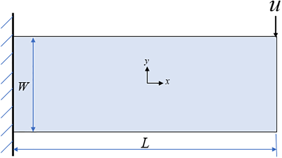
Figure 15: Geometry and boundary conditions of the 2D cantilever beam

To present the simulation results in a more intuitive way, a comparative analysis of the displacements along the beam’s upper and lower edges, visualized using the proposed method and FEM, was performed (see Fig. 16). It can be seen that the statistics robustly proved the reliability of the PD plastic model. Fig. 17a depicts the respective von Mises stress distribution, which is in good agreement with the Abaqus simulation. The stress concentration at the loading point is also clearly visible. In addition, the particles with the yielded bonds were highlighted to display the plastic region in the BB-PD model. Since not all the bonds within the horizon yielded at the same time, the number of bonds to be counted was further controlled. When the number of yielded bonds exceeded 35% of the total bonds in the horizon, the particle was characterized as plastic. It can be observed that the respective plastic region is close to that obtained via Abaqus simulations (see Fig. 17b).

Figure 16: Displacement (mm) of the cantilever beam: (a) upper and (b) lower edges

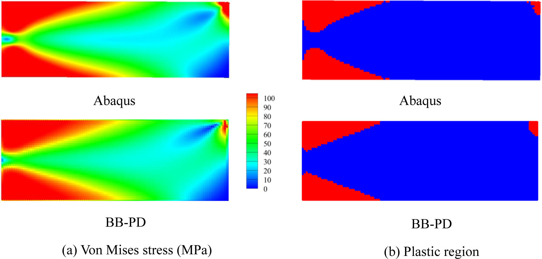
Figure 17: Von Mises stress and plastic region for the cantilever beam

5.4 Fracture Case 1: A Plate with a Pre-Existing Crack

In order to check the fracture criteria and validate the capability of the present model in the prediction of crack propagation, a plate with a central crack under tension was considered. The specimen measured 0.8 m in length and 0.5 m in width. The respective parameters of the material adopted from work [37] are listed in Table 2. The displacement loading in the y-direction was applied to the top and bottom boundaries. A displacement increment was set to 1.0 × 10−3 mm for the peridynamic simulation. The interparticle spacing Δx was 5 mm and the horizon factor was δ=3Δx.

Fig. 18 depicts the crack path of the specimen, obtained experimentally and via PD simulation. The results implied a good agreement between the proposed model and the experiment. The simulated snapshots are shown in Fig. 19, revealing that plastic deformation occurs around the tips of the pre-existing crack. As the displacement load increases, the crack starts to propagate and grow symmetrically along the pre-crack, whereas plastic strain spreads along the newly formed crack surface and the neighboring area. Furthermore, the necking phenomenon can be observed in the middle of the specimen.

Figure 18: Crack path in (a) experiment [37] and (b) the BB-PD model

Figure 19: Damage and plastic strain evolution of the plate with pre-crack

5.5 Fracture Case 2: Kalthoff-Winkler Impacting Test

The Kalthoff-Winkler impacting test [38] is a well-known dynamic failure problem in metallic materials. In the test, a steel plate with two parallel notches is impacted by a projectile to study the failure behavior and characteristics of the material under dynamic conditions. The schematic of the respective experimental setup is given in Fig. 20. The parameters of the material adopted from work [33] are listed in Table 3. The impacting velocity of the projectile is set at 32 m/s.

Figure 20: The setup used in the Kalthoff-Winkler test

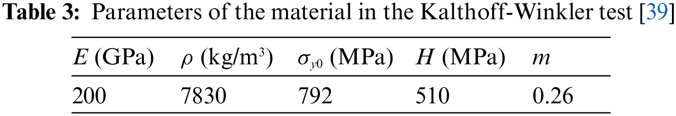
Fig. 21 depicts the crack growth paths and plastic strain obtained using the proposed model. The simulation results indicate that the crack propagates from the notch tip, with a propagation angle of about 69°, which is close to the experimentally found angle of 70° in the study [32]. Plastic deformation can be observed around the crack as well. Given the impact process in Fig. 22a, it can be inferred that the stress wave generated inside the specimen due to the impact gradually propagates downward, then reflects and interacts with the stress wave at the tip, leading to the failure of the region. By comparing the von Mises stress contours during the impact loading, it can be concluded that the present model is in good agreement with that developed by Huang et al. [33] (see Fig. 22b).

Figure 21: Damage and plastic strain evolution in the Kalthoff-Winkler test: (a) crack propagation; (b) plastic strain

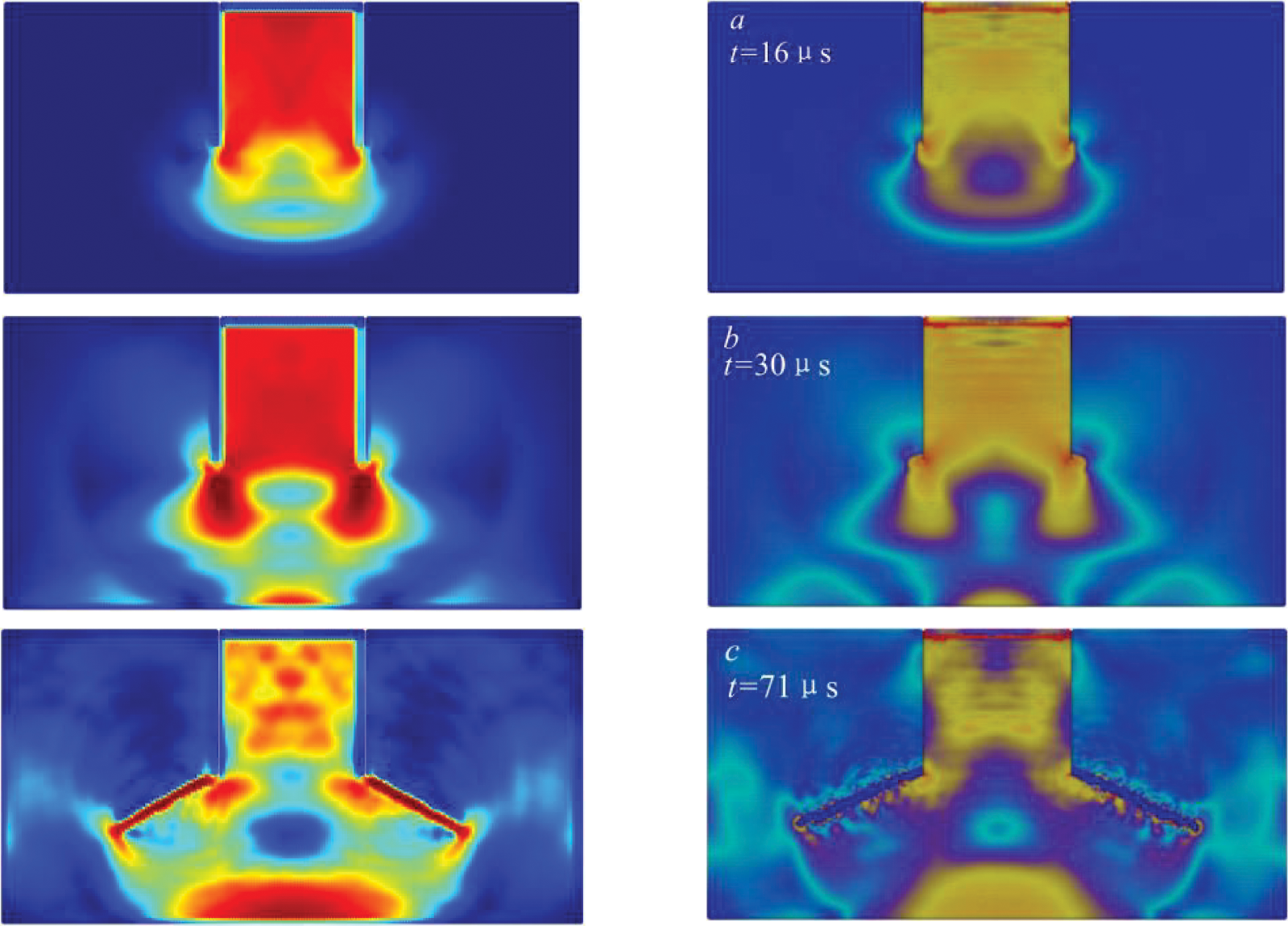
Figure 22: Von Mises stress contours (MPa)

6  Conclusions

In this work, a BB-PD-based model combining plasticity and damage is proposed. The yield condition and flow rule are defined over the pair-wise force function. The numerical algorithm for plastic state update is discussed and provided to demonstrate the validity and performance of the proposed model in fracture and non-fracture problems via both quasi-static and dynamic analyses. The results show that the proposed elastoplastic model provides accurate predictions of materials’ plastic yielding, linear/nonlinear hardening, and fracture behavior. The mechanical response and plastic deformation of macroscopic materials can be captured on the bond level without requiring the introduction of stress and strain concepts of classical mechanics. Therefore, a more straightforward and simplified approach is offered for simulating plastic fracture and expanding BB-PD application. Meanwhile, it is worth noting that the current model is based on the traditional BB-PD framework, which possesses Poisson’s ratio limitation and difficulty in modeling shear-dominated and mixed-mode fractures. The relevant discussion will be further provided in the forthcoming research.

Acknowledgement: The authors acknowledge the supports provided by the National Natural Science Foundation of China. The authors thank anonymous reviewers and journal editors for assistance.

Funding Statement: The corresponding author Lisheng Liu acknowledges the support from the National Natural Science Foundation of China (No. 11972267). The corresponding author Xin Lai acknowledges the support from the National Natural Science Foundation of China (No. 11802214).

Author Contributions: Study conception and design: Lisheng Liu, Yaxun Liu, Liping Zu; formal analysis: Liping Zu, Yaxun Liu, Haoran Zhang; interpretation of results: Liping Zu, Xin Lai; draft manuscript preparation: Liping Zu, Xin Lai; review & editing: Xin Lai, Hai Mei. All authors reviewed the results and approved the final version of the manuscript.

Availability of Data and Materials: No new data were generated or analysed in support of this research.

Conflicts of Interest: The authors declare that they have no conflicts of interest to report regarding the present study.

References

1. Rabczuk T, Belytschko T. Cracking particles: a simplified meshfree method for arbitrary evolving cracks. Int J Numer Meth Eng. 2004;61(13):2316–43. [Google Scholar]

2. Zhang YM, Zhuang XM. Cracking elements: a self-propagating strong discontinuity embedded approach for quasi-brittle fracture. Finite Elem Anal Des. 2018;144:84–100. doi:10.1016/j.finel.2017.10.007. [Google Scholar] [CrossRef]

3. Silling SA. Reformulation of elasticity theory for discontinuities and long-range forces. J Mech Phys Solids. 2000;48(1):175–209. [Google Scholar]

4. Oh M, Koo B, Kim JH, Cho S. Shape design optimization of dynamic crack propagation using peridynamics. Eng Fract Mech. 2021;152(2):107837. [Google Scholar]

5. Wang LW, Sheng XY, Luo JB. A peridynamic damage-cumulative model for rolling contact fatigue. Theor Appl Fract Mech. 2022;121:103489. [Google Scholar]

6. Chu BF, Liu QW, Liu LS, Lai X, Mei H. A rate-dependent peridynamic model for the dynamic behavior of ceramic materials. Comput Model Eng Sci. 2020;124(1):151–78. doi:10.32604/cmes.2020.010115. [Google Scholar] [CrossRef]

7. Liu YX, Liu LS, Mei H, Liu QW, Lai X. A modified rate-dependent peridynamic model with rotation effect for dynamic mechanical behavior of ceramic materials. Comput Methods Appl Mech Eng. 2022;388(24):114246. [Google Scholar]

8. Li S, Lai X, Liu LS. Peridynamic modeling of brittle fracture in mindlin-reissner shell theory. Comput Model Eng Sci. 2022;131(2):715–46. doi:10.32604/cmes.2022.018544. [Google Scholar] [CrossRef]

9. Fan YM, You HQ, Tian XC, Yang X, Li XJ, Prakash N, et al. A meshfree peridynamic model for brittle fracture in randomly heterogeneous materials. Comput Methods Appl Mech Eng. 2022;399(9):115340. [Google Scholar]

10. Madenci E, Barut A, Futch M. Peridynamic differential operator and its applications. Comput Methods Appl Mech Eng. 2016;304:408–51. doi:10.1016/j.cma.2016.02.028. [Google Scholar] [CrossRef]

11. Rabczuk T, Ren H, Zhuang X. A nonlocal operator method for partial differential equations with application to electromagnetic waveguide problem. Comput Mater Contin. 2019;59(1):31–55. doi:10.32604/cmc.2019.04567. [Google Scholar] [CrossRef]

12. Ren H, Zhuang X, Rabczuk T. Dual-horizon peridynamics: a stable solution to varying horizons. Comput Methods Appl Mech Eng. 2017;318:762–82. doi:10.1016/j.cma.2016.12.031. [Google Scholar] [CrossRef]

13. Silling SA, Epton M, Weckner O, Xu J, Askari E. Peridynamic states and constitutive modeling. J Elasticity. 2007;88(2):151–84. [Google Scholar]

14. Madenci E, Oterkus S. Ordinary state-based peridynamics for plastic deformation according to von Mises yield criteria with isotropic hardening. J Mech Phys Solids. 2016;86:192–219. doi: 10.1016/j.jmps.2015.09.016. [Google Scholar] [CrossRef]

15. Liu ZM, Bie YH, Cui ZQ, Cui X. Ordinary state-based peridynamics for nonlinear hardening plastic materials’ deformation and its fracture process. Eng Fract Mech. 2022;223:106782. doi:10.1016/j.engfracmech.2019.106782. [Google Scholar] [CrossRef]

16. Zhou XP, Zhang T, Qian QH. A two-dimensional ordinary state-based peridynamic model for plastic deformation based on Drucker-Prager criteria with non-associated flow rule. Int J Rock Mech Min Sci. 2021;146:104857. doi:10.1016/j.ijrmms.2021.104857. [Google Scholar] [CrossRef]

17. Mousavi F, Jafarzadeh S, Bobaru F. An ordinary state-based peridynamic elastoplastic 2D model consistent with J2 plasticity. Int J Solids Struct. 2021;229:111146. doi:10.1016/j.ijsolstr.2021.111146. [Google Scholar] [CrossRef]

18. Zhang J, LiuX, and Yang QS. A unified elasto-viscoplastic peridynamics model for brittle and ductile fractures under high-velocity impact loading. Int J Impact Eng. 2022;173:104471. doi:10.1016/j.ijimpeng.2022.104471. [Google Scholar] [CrossRef]

19. Kazemi SR. Plastic deformation due to high-velocity impact using ordinary state-based peridynamic theory. Int J Impact Eng. 2020;137(5):103470. [Google Scholar]

20. Lai X, Liu LS, Li SF, Zeleke M, and Wang Z. A non-ordinary state-based peridynamics modeling of fractures in quasi-brittle materials. Int J Impact Eng. 2018;111:130–46. doi:10.1016/j.ijimpeng.2017.08.008. [Google Scholar] [CrossRef]

21. Amani J, Oterkus E, Areias P, Zi G, Nguyen-Thoi T, Rabczuk T. A non-ordinary state-based peridynamics formulation for thermoplastic fracture. Int J Impact Eng. 2016 Jan 1;87:83–94. doi:10.1016/j.ijimpeng.2015.06.019. [Google Scholar] [CrossRef]

22. Zhou XP, Shou YD, Berto F. Analysis of the plastic zone near the crack tips under the uniaxial tension using ordinary state-based peridynamics. Fatigue Fract Eng Mater Struct. 2018;41(5):1159–70. [Google Scholar]

23. Macek RW, Silling SA. Peridynamics via finite element analysis. Finite Elem Anal Des. 2007;43(15):1169–78. [Google Scholar]

24. Chen Z, Wan J, Xiu CX, Chu XH, and Guo XY, “A bond-based correspondence model and its application in dynamic plastic fracture analysis for quasi-brittle materials,” Theor Appl Fract Mech. 2021;113(1):102941. [Google Scholar]

25. Ladányi G, Jenei I. Analysis of plastic peridynamic material with RBF meshless method. Pollack Period. 2008;3(3):65–77. [Google Scholar]

26. Yu HT, Chen XZ, Sun YQ. A generalized bond-based peridynamic model for quasi-brittle materials enriched with bond tension-rotation-shear coupling effects. Comput Methods Appl Mech Eng. 2020;372:113405. doi:10.1016/j.cma.2020.113405. [Google Scholar] [CrossRef]

27. Silling SA, Askari E. A meshfree method based on the peridynamic model of solid mechanics. Comput Struct. 2005;83(17–18):1526–35. [Google Scholar]

28. Sheikhbahaei P, Mossaiby F, Shojaei A. Analyzing cyclic loading behavior of concrete structures: a peridynamic approach with softening models and validation. Theor Appl Fract Mech. 2023;128:104165. doi:10.1016/j.tafmec.2023.104165. [Google Scholar] [CrossRef]

29. Du WJ, Fu XD, Sheng Q, Chen J, and ZhangZP. Study on the failure process of rocks with closed fractures under compressive loading using improved bond-based peridynamics. Eng Fract Mech. 2020;240:107315. doi:10.1016/j.engfracmech.2020.107315. [Google Scholar] [CrossRef]

30. Zhang XX, Ding JG, Zhang Y. A rate-dependent peridynamic model of reinforced concrete subjected to explosive loading. Eng Fract Mech. 2023;292:109666. doi:10.1016/j.engfracmech.2023.109666. [Google Scholar] [CrossRef]

31. Yang D, He X, Liu X, Deng Y, Huang X. A peridynamics-based cohesive zone model (PD-CZM) for predicting cohesive crack propagation. Int J Mech Sci. 2020;184:105830. doi:10.1016/j.ijmecsci.2020.105830. [Google Scholar] [CrossRef]

32. Sheikhbahaei P, Mossaiby F, Shojaei A. An efficient peridynamic framework based on the arc-length method for fracture modeling of brittle and quasi-brittle problems with snapping instabilities. Comput Math Appl. 2023;136:165–90. doi:10.1016/j.camwa.2023.02.020. [Google Scholar] [CrossRef]

33. Ha YD, Bobaru F. Studies of dynamic crack propagation and crack branching with peridynamics. Int J Fract. 2010;162(1–2):229–44. [Google Scholar]

34. Madenci E, Oterkus E. Peridynamic theory and its applications. New York: Springer; 2014. [Google Scholar]

35. Zhang QC, Nguyen-Thanh N, Li W, Zhang AM, Li S, Zhou K. A coupling approach of the isogeometric-meshfree method and peridynamics for static and dynamic crack propagation. Comput Methods Appl Mech Eng. 2023;410:115904. doi:10.1016/j.cma.2023.115904. [Google Scholar] [CrossRef]

36. Li J, Li SF, Lai X, Liu LS. Peridynamic stress is the static first Piola-Kirchhoff virial stress. Int J Solids Struct. 2022;241:111478. doi:10.1016/j.ijsolstr.2022.111478. [Google Scholar] [CrossRef]

37. Simonsen BC, Toernqvist R. Experimental and numerical modelling of ductile crack propagation in large-scale shell structures. Mar Struct. 2024;17(1):1–27. [Google Scholar]

38. Belytschko T, Chen H, Xu J, and Zi G. Dynamic crack propagation based on loss of hyperbolicity and a new discontinuous enrichment. Int J Numer Meth Eng. 2003;58(12):1873–1905. doi:10.1002/nme.941. [Google Scholar] [CrossRef]

39. Wang H, Xu YP, Huang D. A non-ordinary state-based peridynamic formulation for thermo-visco-plastic deformation and impact fracture. Int J Mech Sci. 2019;159:336–44. doi:10.1016/j.ijmecsci.2019.06.008. [Google Scholar] [CrossRef]

Appendix

Method of Stress Calculation in Bond-Based Peridynamics

According to Li et al. [36], the peridynamic Cauchy stress tensor can be calculated as

P(x)=12Ωx(∑i=1Nx∑j=1,j≠iNxtij⊗(xj−xi)),xi,xj∈Hx

where Ωx is the horizon volume; xi and xj are the relative positions of the particles in the current configuration; tij is the force between the particles, which is defined as

tij=12fijViVj

where Vi,Vj are the volumes of particles i and j.

The von Mises stress can be obtained as follows:

σ¯=12(σx−σy)2+(σy−σx)2+(σz−σx)2+6(τxy+τyz+τzx)2