
 Submit a Paper
 Propose a Special lssue
 Open Access
ARTICLE
A Novel ISSA–DELM Model for Predicting Rock Mass Permeability
1 School of Engineering and Technology, China University of Geosciences (Beijing), Beijing, 100083, China
2 Beijing Engineering Corporation Limited, Beijing, 100024, China
* Corresponding Author: Leihua Yao. Email:
Computer Modeling in Engineering & Sciences 2024, 140(3), 2825-2848. https://doi.org/10.32604/cmes.2024.049330
Received 03 January 2024; Accepted 10 May 2024; Issue published 08 July 2024
 View Full Text
 Download PDF
Abstract
In pumped storage projects, the permeability of rock masses is a crucial parameter in engineering design and construction. The rock mass permeability coefficient (K) is influenced by various geological parameters, and previous studies aimed to establish an accurate relationship between K and geological parameters. This study uses the improved sparrow search algorithm (ISSA) to optimize the parameter settings of the deep extreme learning machine (DELM), constructing a prediction model with flexible parameter selection and high accuracy. First, the Spearman method is applied to analyze the correlation between geological parameters. A sample database is built by comprehensively selecting four geological indexes: burial depth, rock quality designation (RQD), fracture density characteristic index (FD), and rock mass integrity designation (RID). Hence, the defects of the sparrow search algorithm (SSA) are enhanced using the improved strategy, and the initial input weights of the DELM are optimized. Finally, the proposed ISSA–DELM model is employed to predict the permeability coefficient of rock mass in the entire study area. The results showed that the predictive performance of the model is superior to that of the DELM and SSA–DELM. Therefore, this model successfully provides insights into the distribution characteristics of rock mass permeability at engineering sites.Keywords
Nomenclature
| ISSA | Improved sparrow search algorithm |
| DELM | Deep extreme learning machine |
| RQD | Rock quality designation |
| FD | Fracture density characteristic index |
| RID | Rock mass integrity designation |
| K | Rock mass permeability coefficient |
K is vital for quantitatively describing the flow and migration of groundwater in rock fissures. It is an essential index for engineering anti-seepage design and hydrogeological evaluation [1,2]. Therefore, an accurately determined permeability of rock masses is a prerequisite for the structural design, construction feedback, and stability analysis of tunnels. K is influenced by various geological parameters, such as rock mass integrity, fracture structure, and rock mass quality [3–5]. Some researchers have explored the relationship between various factors and rock mass permeability. Piscopo et al. [6] analyzed the relationship between discontinuous spacing, depth, and permeability of a rock mass and determined the preliminary characteristics of rock mass in a study area. Pei et al. [7] established a predictive model for K at highly radioactive waste disposal sites using rock mechanics parameters. The existing studies focus on inflexible parameter selection and difficulty in obtaining parameters.
Due to the heterogeneity and anisotropy of rock masses, K can exhibit substantial spatial variability, resulting in difficulty in accurately obtaining its value. The primary methods utilized to determine K include field hydrogeological tests, empirical formula methods, and numerical seepage simulations [8–10]. The permeability coefficients obtained from field tests are the most direct and effective. However, owing to the limitations in geological conditions and the construction period, only a small amount of data can be obtained in crucial areas, making it impossible to display the distribution characteristics of rock mass permeability. In the empirical formula method, the possible nonlinear relationship between the parameters and permeability coefficient can result in significant errors in the calculation results. The numerical simulation method requires many calculations, requires considerable time and cost, and does not consider the correlation between numerous input parameters. Therefore, a suitable method to accurately evaluate rock-mass permeability is urgently required.
Establishing complex nonlinear relationships involves predicting K using various geological parameters. Machine learning algorithms have advantages in solving these nonlinear problems and provide essential methods of obtaining the value of K quickly and efficiently [11–13]. Extreme learning machine (ELM) has advantages such as high computation speed and a simple structure [14]. Deep extreme learning machine (DELM) extends ELM to multilayer structures, which can better mine the basic features of data and improve the generalization ability of a model [15]. However, the initial weighting of the DELM depends on random selection, which can affect the training process in terms of accuracy and time consumption [16]. Researchers typically use swarm intelligence optimization algorithms to optimize objective parameters to avoid this limitation [17–19]. The sparrow search algorithm (SSA) has been shown to have excellent search capabilities [20,21]. The random input weights and random deviations of the DELM have been optimized using the SSA, which can significantly improve the accuracy of DELM. However, the standard SSA tends to fall into local optima in later iteration stages [22]. Mao et al. [23] proposed an improved sparrow search algorithm (ISSA) that combines Cauchy mutations and opposition-based learning (OBL), which enhanced its ability to resist local optima. Qiao et al. [24] improved the basic SSA using a firefly algorithm and optimized the initial input weights of the DELM. Therefore, using various optimization algorithms can improve the prediction accuracy and efficiency of the DELM.
Accordingly, this study selects geological parameters that are easy to obtain and crucial in engineering sites to represent the permeability characteristics of rock masses at an engineering site as accurately as possible. The correlation between these parameters and K is analyzed in detail, and a dataset of characteristic variables in the engineering site is constructed. Hence, the basic SSA is enhanced based on the improvement strategy, and an ISSA–DELM model integrating multiple factors is constructed to predict the distribution pattern of the permeability coefficients in the engineering site. This model can provide guidance for the design of engineering structural supports and the analysis of the surrounding rock stability.
DELM is an ELM-derived method that constructs multilayer network structures by superimposing an extreme learning machine auto-encoder (ELM-AE) to minimize input information reconstruction errors and improve the representational capability of a network. The output of the ELM-AE is expressed as follows:
where a is a matrix composed of
When m > L, the ELM-AE can achieve dimensional compression, which transforms the input data with high dimensionality into a feature space with low dimensionality, whereas when m < L, the ELM-AE can achieve sparse representation, indicating that the input data are converted from a low-dimensional to a high-dimensional expression space. The output weight β for the ELM-AE is described in Eq. (2). If m = L, the ELM-AE can achieve a feature expression of equal dimensionality, as depicted in Eq. (3). In each case, the objective of the ELM-AE is to learn a feature representation through which the original data can be efficiently reproduced or transformed into new and valuable feature forms.
where X = [X1, X2, X3, …, XN] is the input data; C is the regularization parameter; H is the hidden layer output matrix of the ELM-AE; I is the unit matrix.
In the training process of the DELM, the original data sample X is typically employed as the output of the first ELM-AE layer (X = X1) to obtain the output weight β1. Hence, the output matrix H1 of the first hidden layer in the DELM method is used as the input of the second ELM-AE layer (X = X2), and so on, layer by layer. The network structure model of the DELM is shown in Fig. 1.
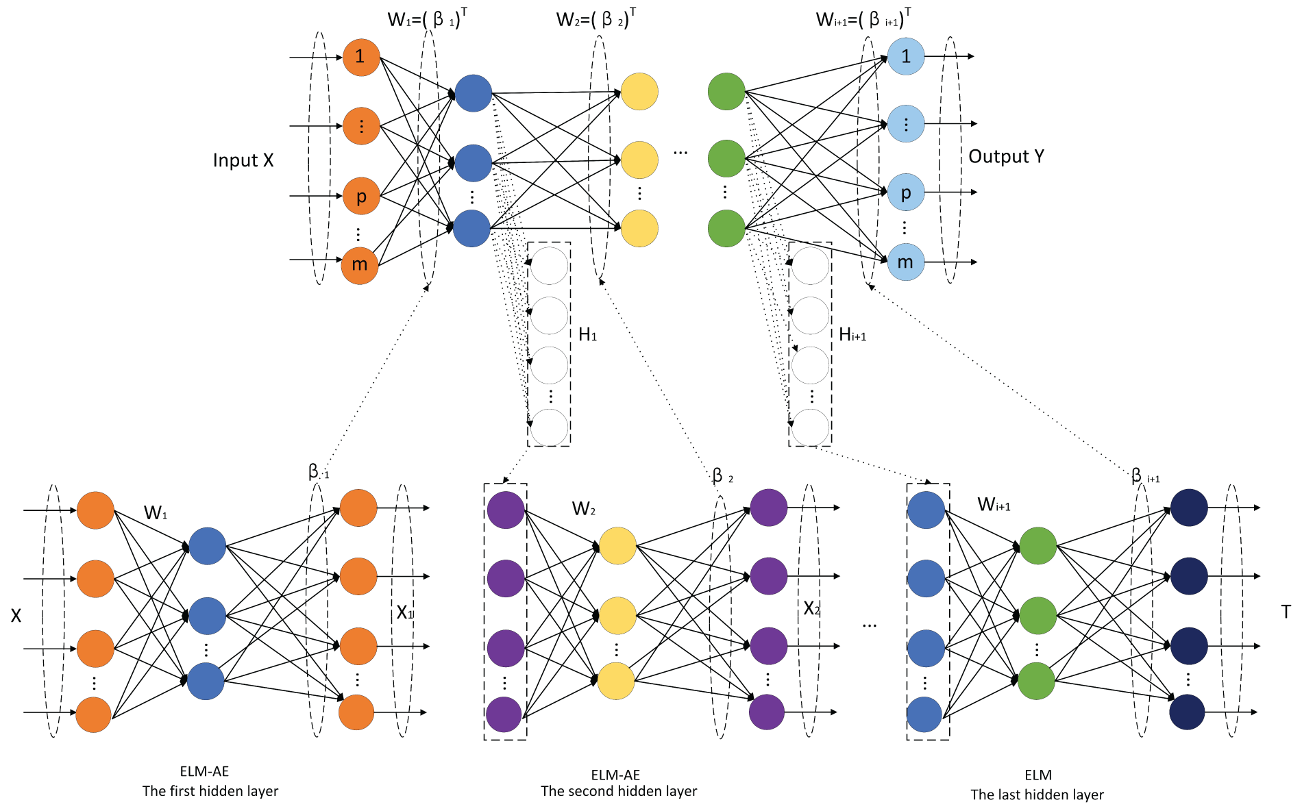
Figure 1: Network structure model of the DELM
The SSA is a relatively new swarm intelligence optimization algorithm introduced in 2020 [21]. This algorithm is mainly inspired by sparrows’ foraging and anti-feeding behaviors and has advantages such as strong optimization ability and fast convergence. The sparrows in the SSA are divided into discoverers and joiners, which change dynamically. The position of the discoverer is updated as follows:
where
If discoverers find food, they instantly leave their present position to compete. The position update equation for joiners is expressed as follows:
where
When a population forages, sparrows provide alerts. Vigilantes are randomly generated in each group. The initial positions are randomly generated using the following rules:
where Xbest is the global best position; β is a step control parameter; K is a uniform random number in the range [−1, 1] and represents the direction of the sparrow movement;
Mao et al. [23] presented an ISSA combining Cauchy’s variant and backward learning to address the decreasing population diversity of SSA and its tendency to fall into local optimization in later iterations. The algorithm improves the global optimization performance of the SSA through several strategies.
(1) Sine chaotic initialization
Sine and logistic chaos are typically employed to improve the optimization performance of search problems. When the sine chaotic method initializes the population, it ensures that the entire sparrow population is uniformly distributed throughout the search space, thus increasing the probability of determining the globally optimal solution [25]. Yang et al. [26] observed that sine chaos exhibits superior chaotic properties to logistic chaos. Therefore, sine chaos has advantages as a method of initializing the population in the SSA, and its one-dimensional self-mapping formula is expressed as follows:
The initial value cannot be 0 to prevent immobility and the occurrence of a zero point at [−1, 1].
(2) Dynamic adaptive weights
This study proposes an improved discovery position update strategy to enhance the effectiveness of the search algorithm and avoid prematurely falling into local optimal solutions. The advantage of this method is that the discoverer not only considers their previous position when moving but is also guided by the previously determined optimal solution. This aids the algorithm in breaking out potential local optimal traps determined solely by their current position [22]. In addition, this study incorporates a dynamic weight factor ω [27], which adaptively adjusts its size with the iteration process. Thus, the algorithm can maintain a large displacement during the initial exploration stage and gradually enhance convergence during the process of obtaining accurate solutions. The formulas for the weight factor ω and updating the discoverer position are shown below:
where
The updated formula for the improved vigilantes is
The improved equation indicates that when a sparrow is in the optimal position in a group, any point between the current optimal and worst positions is selected as the new foothold to avoid potential danger or prevent resource depletion. In other cases, a random point is selected to jump between its current and best positions.
(3) Integration of Cauchy mutation and OBL
The use of Cauchy mutation can introduce more variation into the population to improve the ability of the algorithm to explore the entire search space.
Incorporating Cauchy mutations into the update process of the target search positions further expands the algorithm’s performance in global optimization problems.
The OBL method [28] was integrated into the SSA to enhance the algorithm’s exploration efficiency during optimization. The formula is expressed as follows:
The optimization efficiency of the algorithm is improved through a flexible selection mechanism that dynamically switches between different strategies [23]. The algorithm selects between OBL and Cauchy mutation operators to update the target solution, depending on the selection probability
where
If
Although OBL and Cauchy mutations can help the algorithm avoid falling into local optima, each perturbation or variation is not guaranteed to result in a better solution because they are stochastic. Therefore, the algorithm introduces a greedy rule to overcome the possible degradation of the solutions caused by random disturbances. The greedy rule is a selective updating mechanism that ensures that the algorithm only updates its position when it obtains a higher-quality solution. The greedy rule is expressed as follows:
(4) Algorithm performance testing
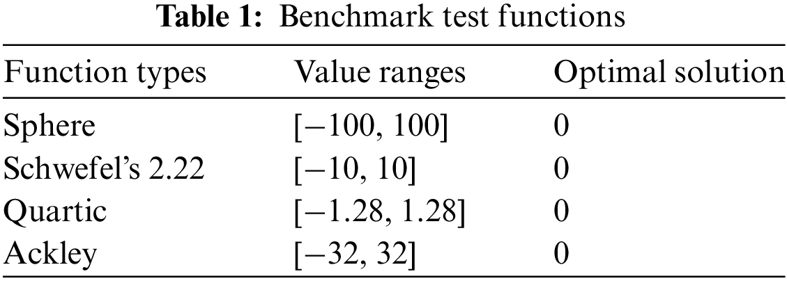
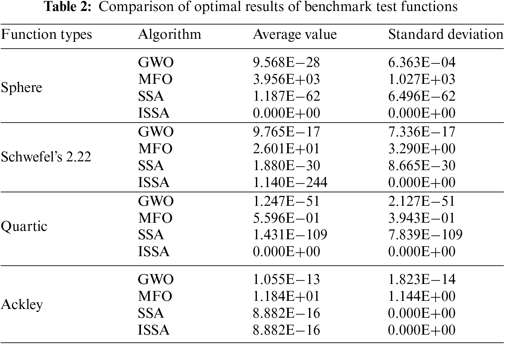
Four benchmark functions are employed to compare the performance of ISSA with SSA, grey wolf optimization (GWO), and moth-flame optimization (MFO) [23]. To reasonably verify the effectiveness of the ISSA algorithm, testing was conducted in the same operating environment. The general conditions are set to the same, with a population size of 30, a dimension of 30, 500 iterations, and each algorithm running independently 50 times. Table 1 lists the specific benchmark function information, whereas Table 2 shows the comparison results. The average value and standard deviation of multiple optimizations compared to the other three algorithms show that the average value calculated by the ISSA algorithm can be close to the theoretical optimal solution, and the standard deviation is the smallest. The results indicate that the stability and robustness of the improved algorithm are better than the other algorithms.
The algorithm steps are as follows:
1. Initialize parameters (Percentage of discoverers (PD), Percentage of vigilantes (SD), warning value (ST), and others) and use Eq. (8) to perform sine chaotic mapping to enrich the population diversity.
2. Calculate the fitness values of each sparrow.
3. Sparrows with better fitness values are selected as discoverers, and their positions are updated according to Eq. (10). The remaining sparrows serve as joiners and update their positions according to Eq. (6). Update the position of the vigilantes according to Eq. (11).
4. Select the Cauchy mutation or OBL strategy based on the Ps to perturb the current optimal solution and generate a new one.
5. Determine whether to perform position updates based on Eq. (17).
6. Determine whether the end condition is satisfied. If the conditions are satisfied, the optimal position of the output sparrow is used as the optimal input weight for the DELM model. Otherwise, skip to step (2).
The input layer weights and thresholds of the DELM are randomly generated from the orthogonal matrices according to the Johnson–Lindensrauss theorem. This orthogonalized design enhances the generalization ability of the system but also results in high volatility in the prediction results. Therefore, the ISSA is used to optimize the input layer weights and thresholds to reduce the prediction model’s volatility and enhance the prediction results’ stability and accuracy. The optimization process and flowchart are depicted in Fig. 2.
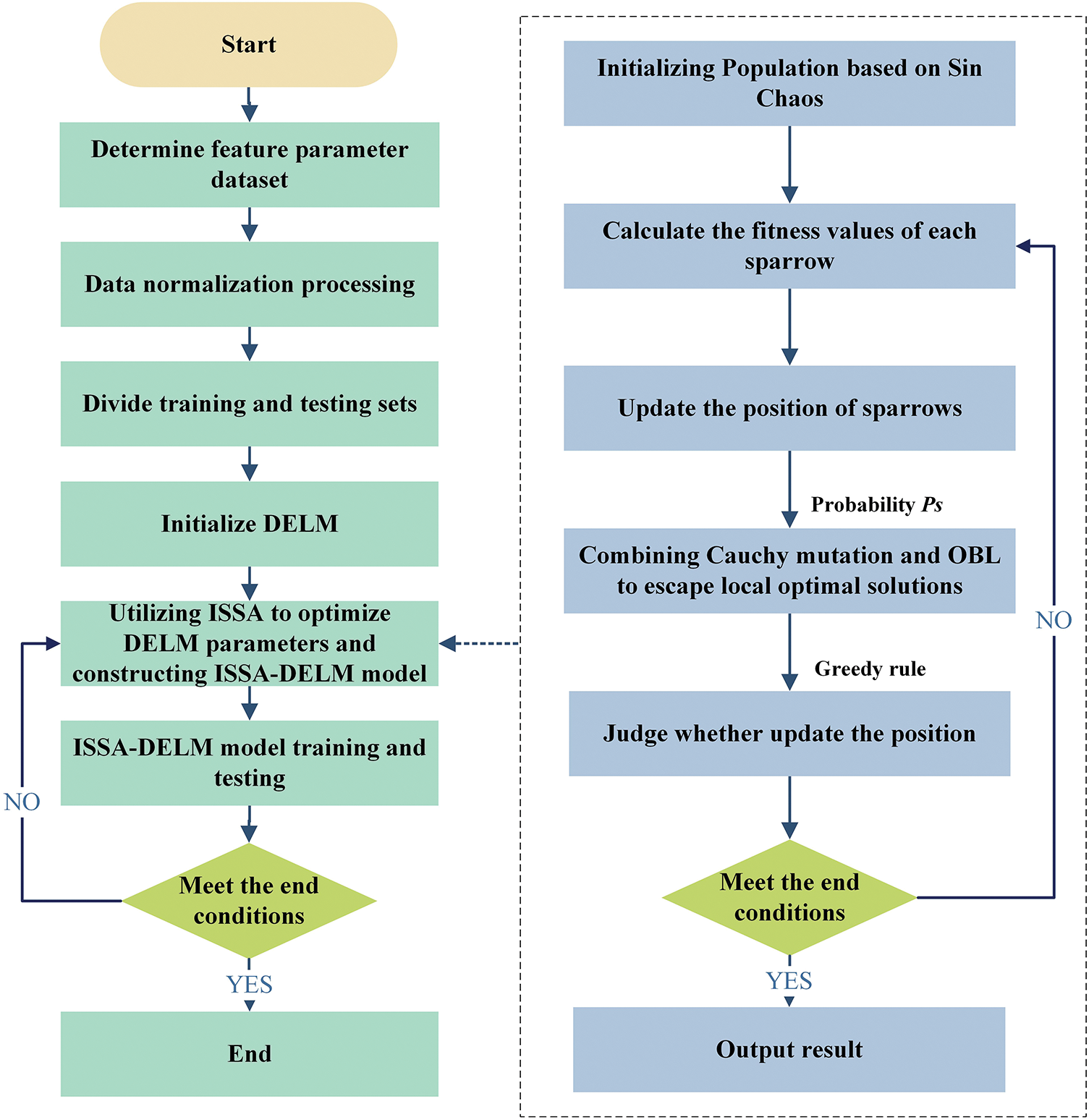
Figure 2: ISSA–DELM flow chart
A pumped-storage power station in Shanxi Province is planned to have an installed capacity of 1500 MW with a first-class engineering grade. The survey and location map of the study area are shown in Fig. 3. This project focuses on serving the northern power grid of Shanxi Province and can provide flexible scheduling and complementary advantages between networks for the North China Power Grid.
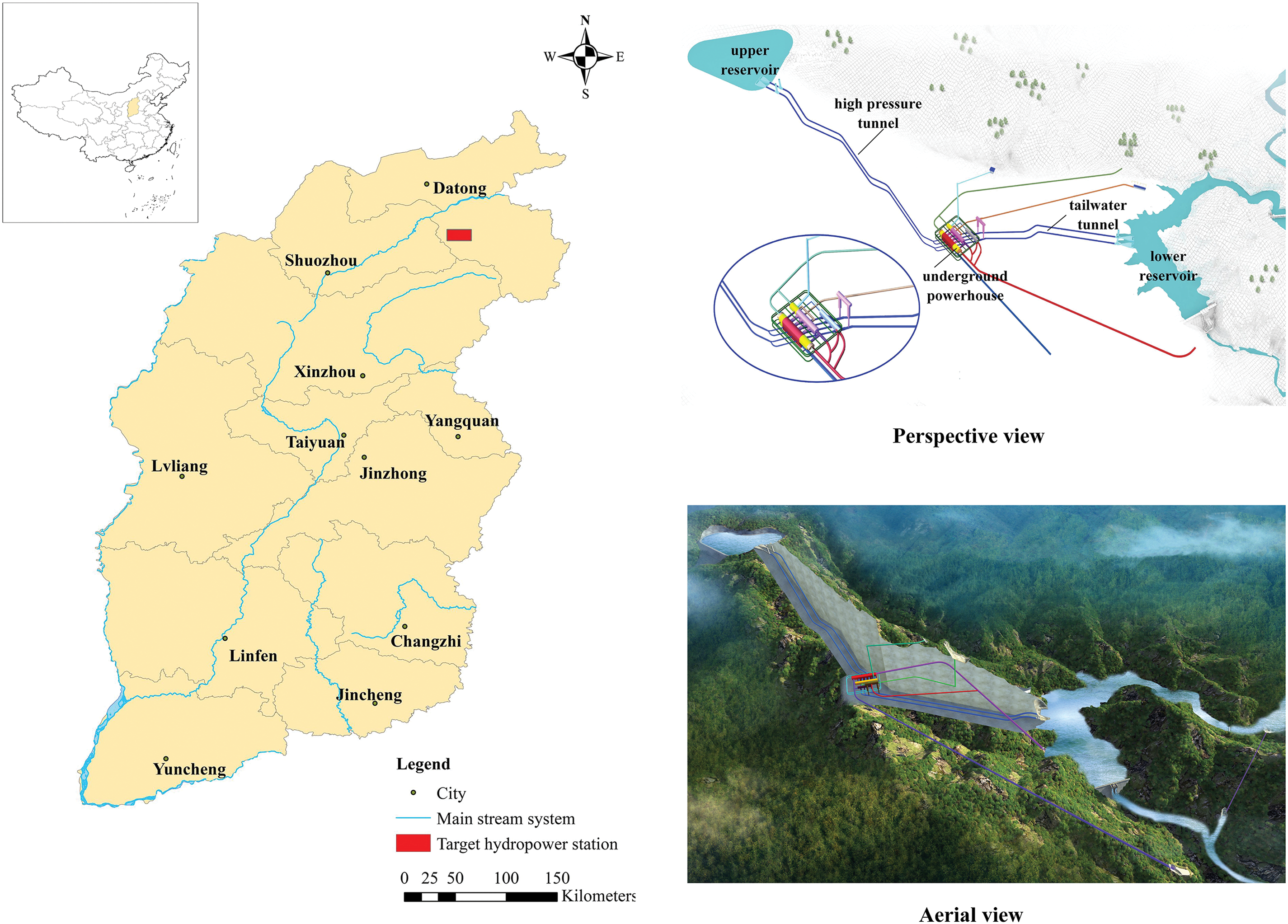
Figure 3: Survey and location map of the studied area
3.2 Engineering Geological Conditions
The geological engineering conditions are shown in Fig. 4. The terrain of the engineering site is high in the east and low in the west, and it belongs to a medium-low mountain landform. The mountaintop elevation is generally 1100–2200 m. The gullies in the area are deeply cut, and the cross sections are mainly in a “V” shape. The lithology is primarily gneiss, and the surrounding rock types are II and III. Based on geological mapping, the surface is affected by in-situ stress and rock unloading, resulting in dense zones of northeast-oriented unloading cracks in multiple locations. The connectivity of the rock fractures is poor, and the rock mass has a certain degree of impermeability. Based on the field water pressure test, the overall permeability of the rock mass in the engineering site ranges from micro to weak permeability. According to the results of acoustic testing, the wave velocity of a Class II rock mass is typically greater than 4500 m/s, whereas the wave velocity of a more complete Class III rock mass is generally between 3500 and 4500 m/s. The groundwater level in the engineering site varies with the terrain, and its depth is generally within the range of 30–100 m.
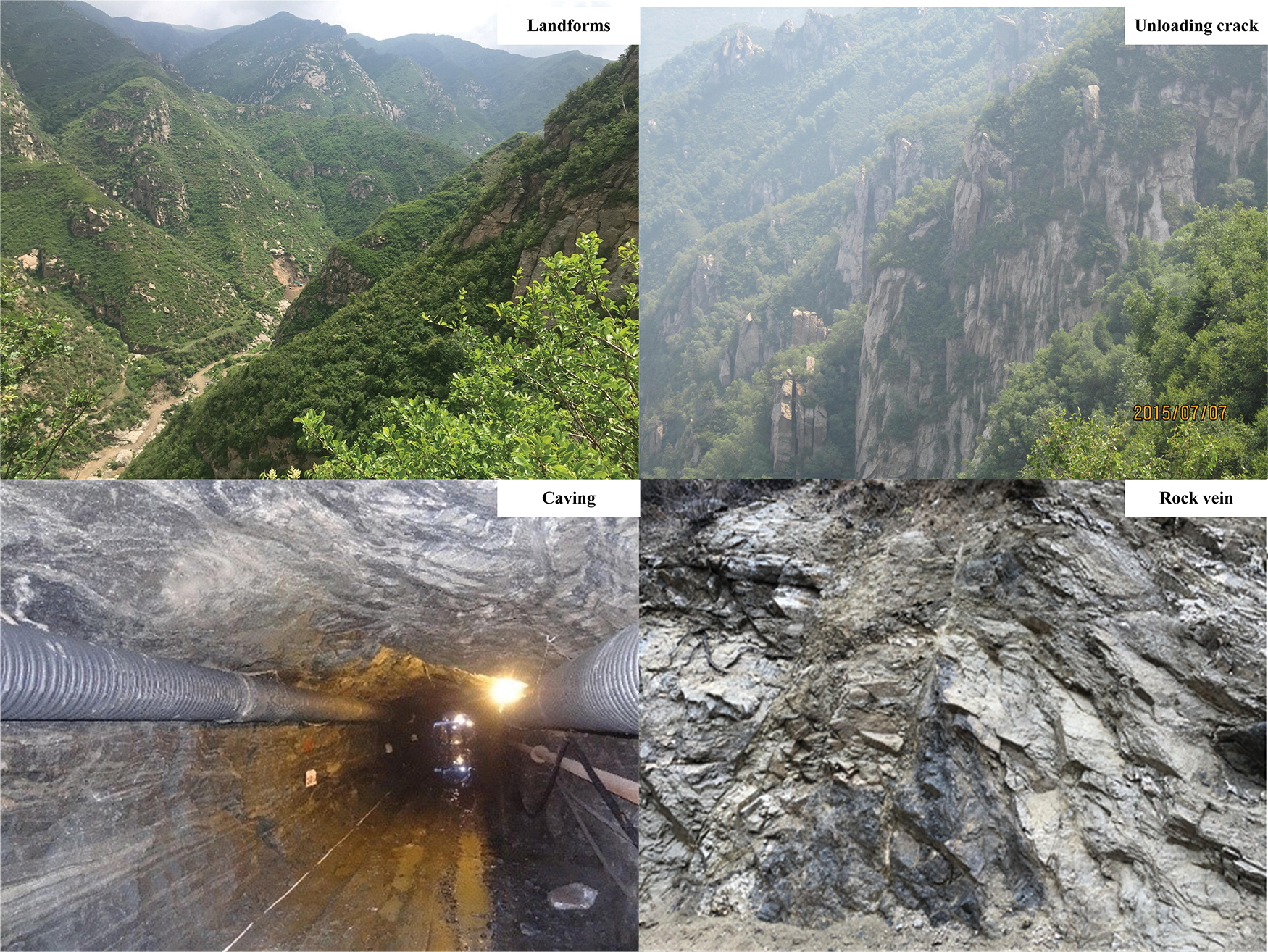
Figure 4: Engineering geological conditions
The burial depth reflects the stress level of the geological environment in which the rock mass is located. K is closely related to the burial depth [30]. Generally, K gradually decreases as the burial depth increases [31]. Several researchers have applied a semi-empirical-semi-theoretical approach to determine the relationship between K and the burial depth. Achtziger-Zupančič et al. [32] established empirical formulas for the variation in K with the burial depth through power functions. Wei et al. [33] established an empirical formula for the variation in K with the burial depth in the form of a hyperbolic function. Accordingly, the burial depth influences almost all methods for estimating K. The distribution pattern of K in the project area with burial depth is shown in Fig. 5. The coefficient K gradually decreases with increasing burial depth within the 0–700 m range. It varies significantly below 100 m, whereas it varies less as the burial depth continues to increase. This indicates a certain degree of spatial variability in the rock mass of the project area.
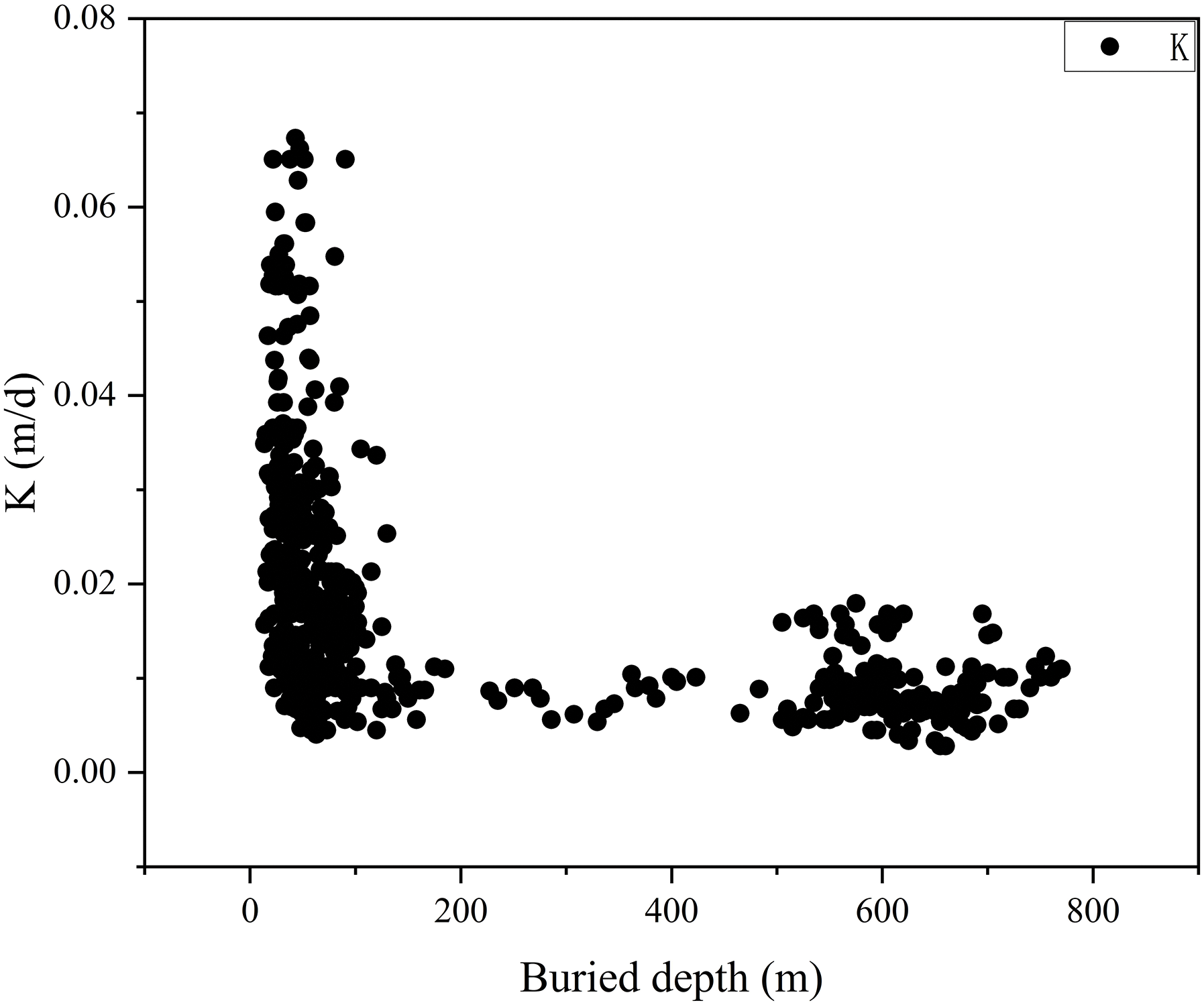
Figure 5: Relationship between burial depth and K
4.1.2 Rock Quality Designation (RQD)
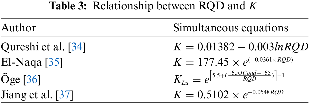
The RQD is a quantitative index of a rock mass’s degree of integrity and weathering. Therefore, several researchers have studied the relationship between the RQD and K, as shown in Table 3. This table shows a negative correlation between RQD and K, indicating that the larger the RQD value, the smaller the K value.
4.1.3 Development and Filling of Rock Masses
The permeability properties of rock masses are influenced by the fracture filling and their developmental characteristics [3,4]. However, the quantitative parameters for filling are challenging to obtain and cannot be widely used in engineering applications. The development characteristic indexes of rock masses can be relatively easily obtained by drilling and employing borehole TV, including the (starting and ending) depth, density, dip angle, tendency, and width of fractures. The density and dip angle of fractures can be obtained directly from the drilling data, which is convenient and time-efficient for engineering applications. As shown in Figs. 6a and 6b, at the same RQD value, the permeability properties of the rock mass changed with different fracture densities (number of strips). Under tectonic stress, the structural plane formed dip angles of varying widths. In particular, steep dip angles (60–90°) significantly affect the RQD. As shown in Figs. 6c and 6d, at constant fracture density, the proportion of steep dip angles varied, affecting the rock mass’s permeability. Accordingly, the different development conditions of the structural planes resulted in different plane characteristics, leading to significant differences in the permeability performance. Therefore, the development indexes of these structural planes should be considered when calculating K.
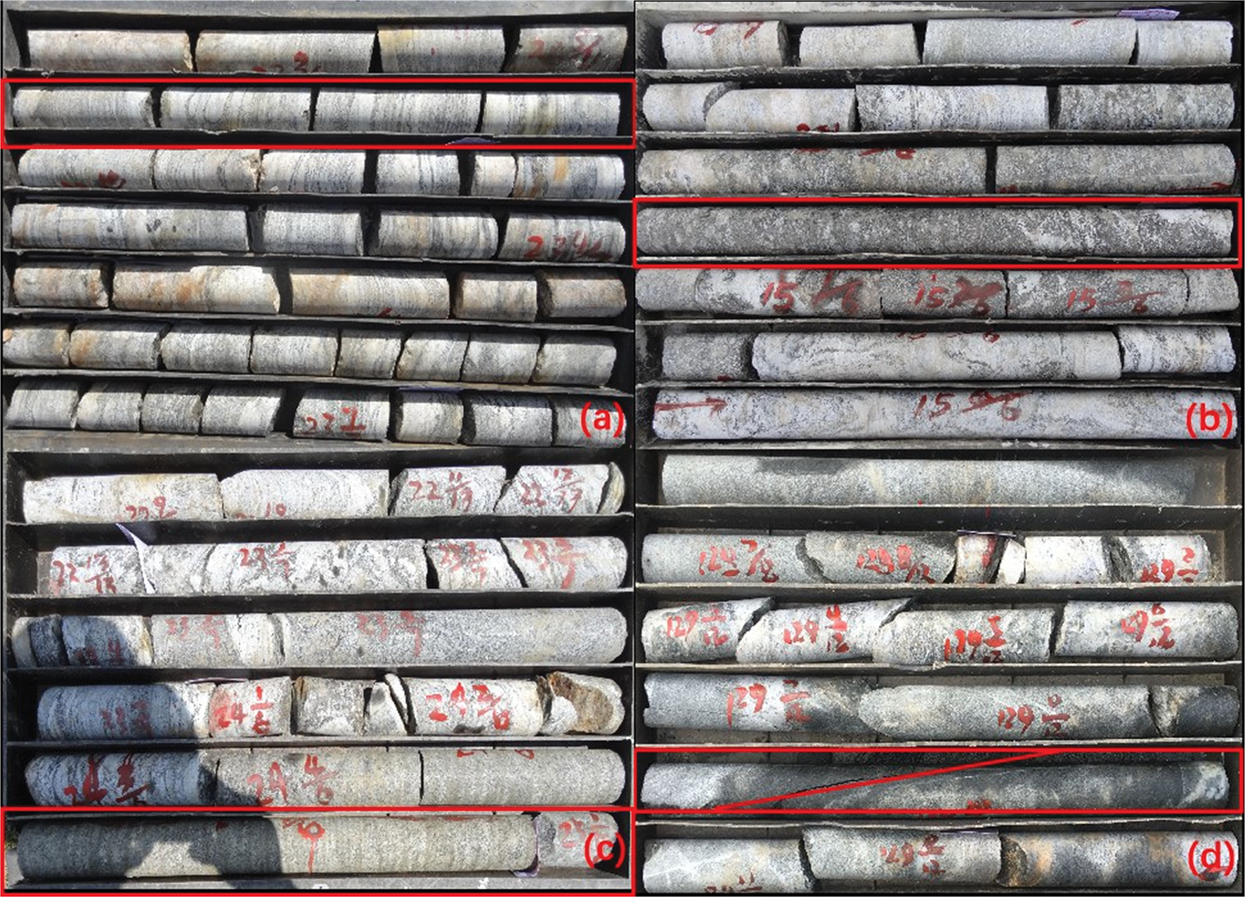
Figure 6: Comparison of the development characteristics
4.1.4 Rock Mass Integrity Designation
The RID represents the integrity index of a rock mass through its longitudinal wave velocity index, as shown in Eq. (18). Fig. 7 depicts that the longitudinal wave velocity of the rock body decreased sharply at a drilling depth of 63–64 m. The corresponding drilling data and TV video indicate that the rock body is considerably damaged and the rock quality is poor, confirming that the longitudinal wave velocity is correlated with the integrity of the rock body. The larger the RID value, the better the integrity of the rock and the lower the permeability coefficient; thus, the index may be negatively correlated with K. If the elastic longitudinal wave velocity of the drilled rock mass is greater than the elastic longitudinal wave velocity of the rock in the laboratory, it will result in a RID greater than 1. Therefore, a relatively complete and homogeneous rock mass section must be selected as the standard sample based on the core and borehole TV. The maximum wave velocity of all the standard samples is selected as the elastic longitudinal wave velocity of the rock [38].
where
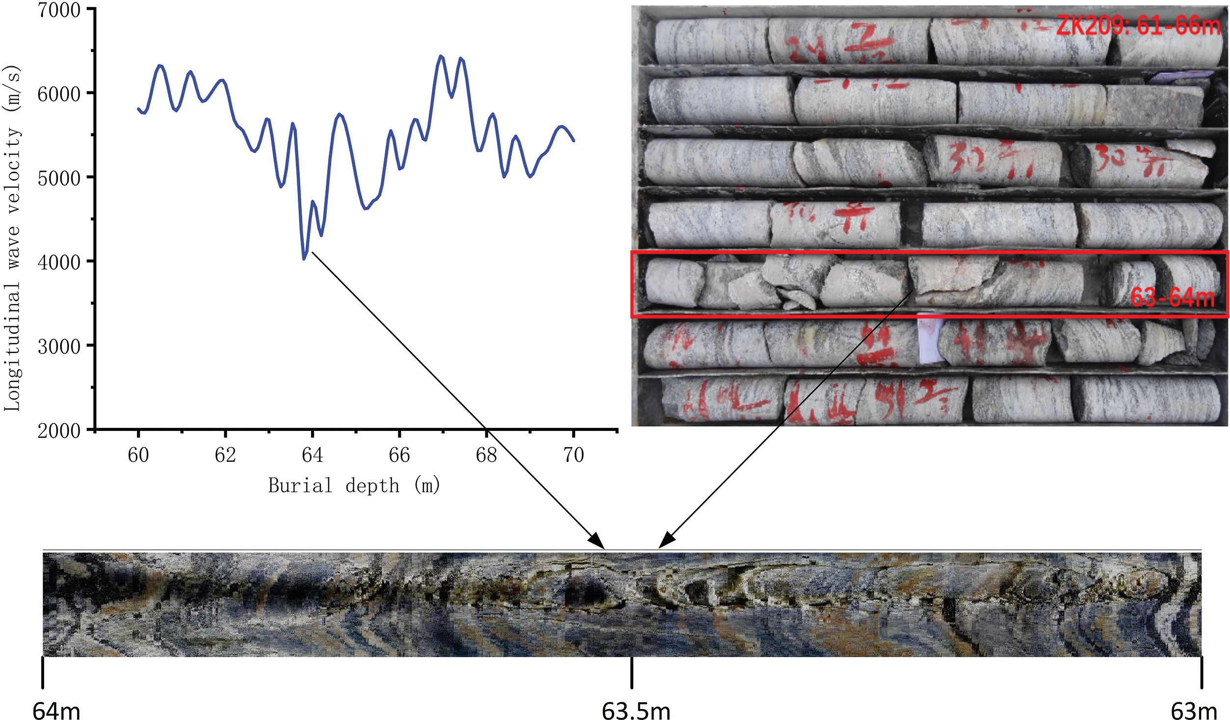
Figure 7: Comparison of acoustic wave velocities with drilling data and TV recordings
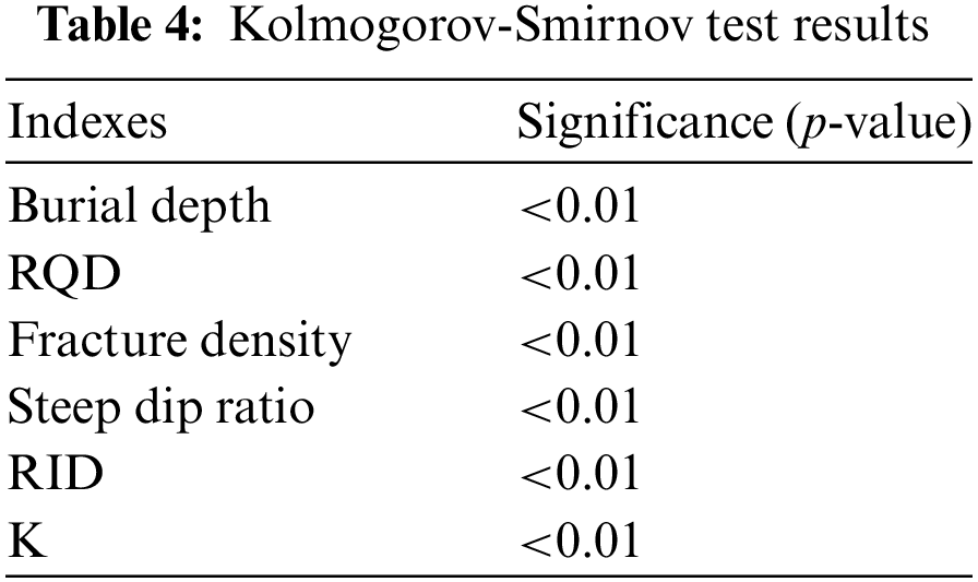
K is affected by several factors. Parameter correlation analysis helps identify and quantify model parameters, providing reference values for parameter optimization and model construction. To further select appropriate correlation analysis methods, this study calculated normality tests on the distribution characteristics of geological parameters using the Kolmogorov-Smirnov test and histograms. Fig. 8 and Table 4 indicate that these data do not follow a normal distribution (p < 0.05) and do not belong to ordered categorical variables. Therefore, the Spearman correlation analysis method is used for index correlation analysis.
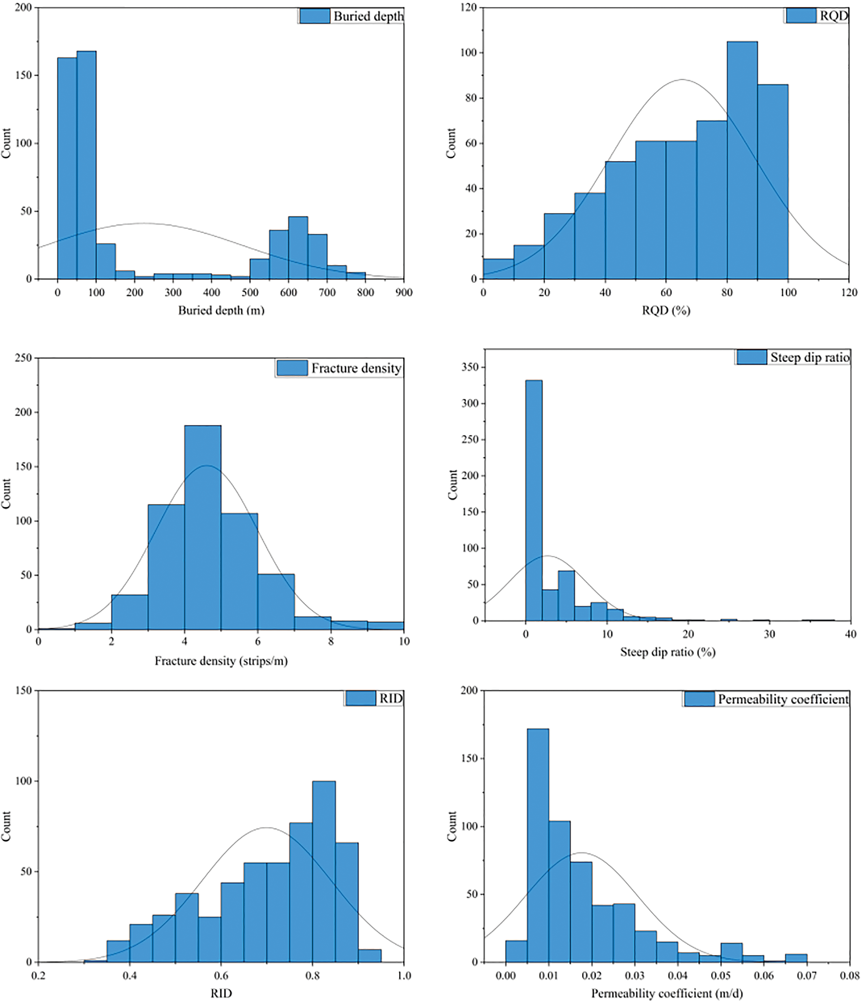
Figure 8: Modeling data histograms
Spearman correlation explores the correlation between continuous variables in the range of [−1, 1]. Fig. 9 demonstrates that the correlation coefficient between the RQD and RID is greater than 0.6, which is a strong positive correlation. It also implied that the better the integrity of the rock mass, the higher the quality of the rock mass. The absolute value of the correlation coefficients between the RQD and RID and fissure density is greater than 0.4, indicating a moderately negative correlation. This also demonstrates that the lower the fracture density of the rock mass, the better the quality and integrity of the rock mass tended to be. The correlation coefficient between the RID, RQD, and burial depth is greater than 0.4, a moderately positive correlation. This indicates that the rock mass’s quality and integrity tend to improve with the increase of burial depth in this project area. In addition, the Spearman correlation analysis between the five geological parameters and K showed that K had a strong negative correlation with the burial depth, RQD, and RID; a moderate positive correlation with the fracture density; and a certain degree of weak positive correlation with the steep dip ratio.
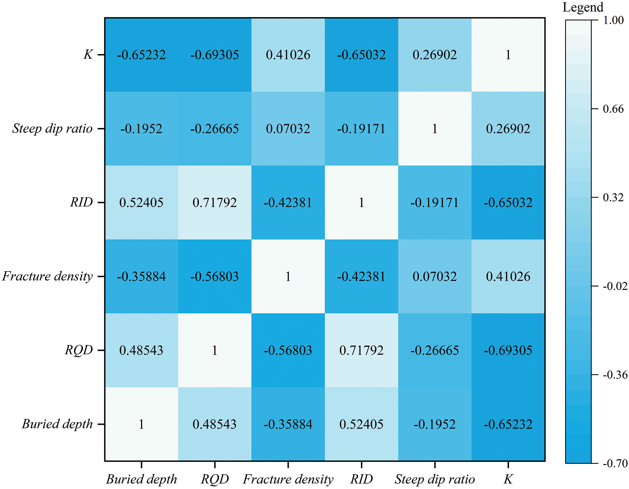
Figure 9: Spearman correlation analysis chart
Due to the limited proportion of steep-dip ratios in the sample data, some deviations can be occurred in the correlation analysis. The lithology of this project area was primarily composed of metamorphic rocks, and the weight of the fracture steep-dip ratio significantly impacted K. Therefore, the direct exclusion of this parameter can impact the predictive analysis results. Based on the lithological characteristics and industry experience, the dip ratio and fracture density were combined to form a fracture density characteristic index abbreviated as FD, which was shown in Eq. (19). Fig. 10 exhibits that the correlation coefficient between FD and K is 0.583, indicating a moderate positive correlation.
where

Figure 10: Optimized Spearman correlation analysis chart
In summary, the permeability of rock masses is closely related to the burial depth, RQD, and degree of fracture development. This study indexes selected geological parameters such as the burial depth, RQD, FD, and RID as the modeling indexes to ensure the model’s accuracy. Hence, a prediction model of the rock mass permeability based on a multi-index was developed to mitigate the problems of inflexible parameter selection and unreasonable model construction.
5.1 Database Construction Process
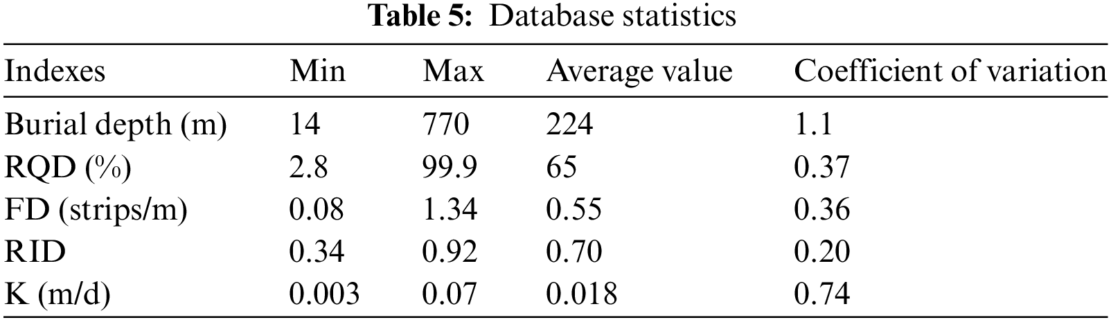
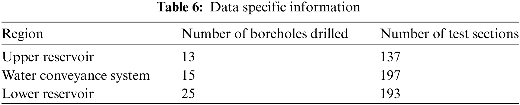
Based on the above analysis, four independent and one dependent variables were selected to form a database. A total of 527 valid samples were collected through field tests, with 88% of the rock mass being slightly weathered. The specific information is presented in Tables 5 and 6. In the input dataset for the geological parameters, the burial depth, RQD, and FD were obtained from borehole data and borehole TV, and the RID parameters were derived by acoustic logging. The permeability coefficient values were obtained in the output dataset using an atmospheric pressure water test. The permeability prediction model constructed in this study applies to parameters such as the Lvrong value, permeability flow rate, and permeability coefficient. This study selected the actual permeability coefficient values from on-site testing to avoid repetition as the prediction index.
The data were divided into two independent datasets: 440 for simulation and 87 for testing the model, as shown in Fig. 11. This study processed the original data using the max-min normalization method to eliminate the effect of dimensionality and improve the algorithm’s performance.
where
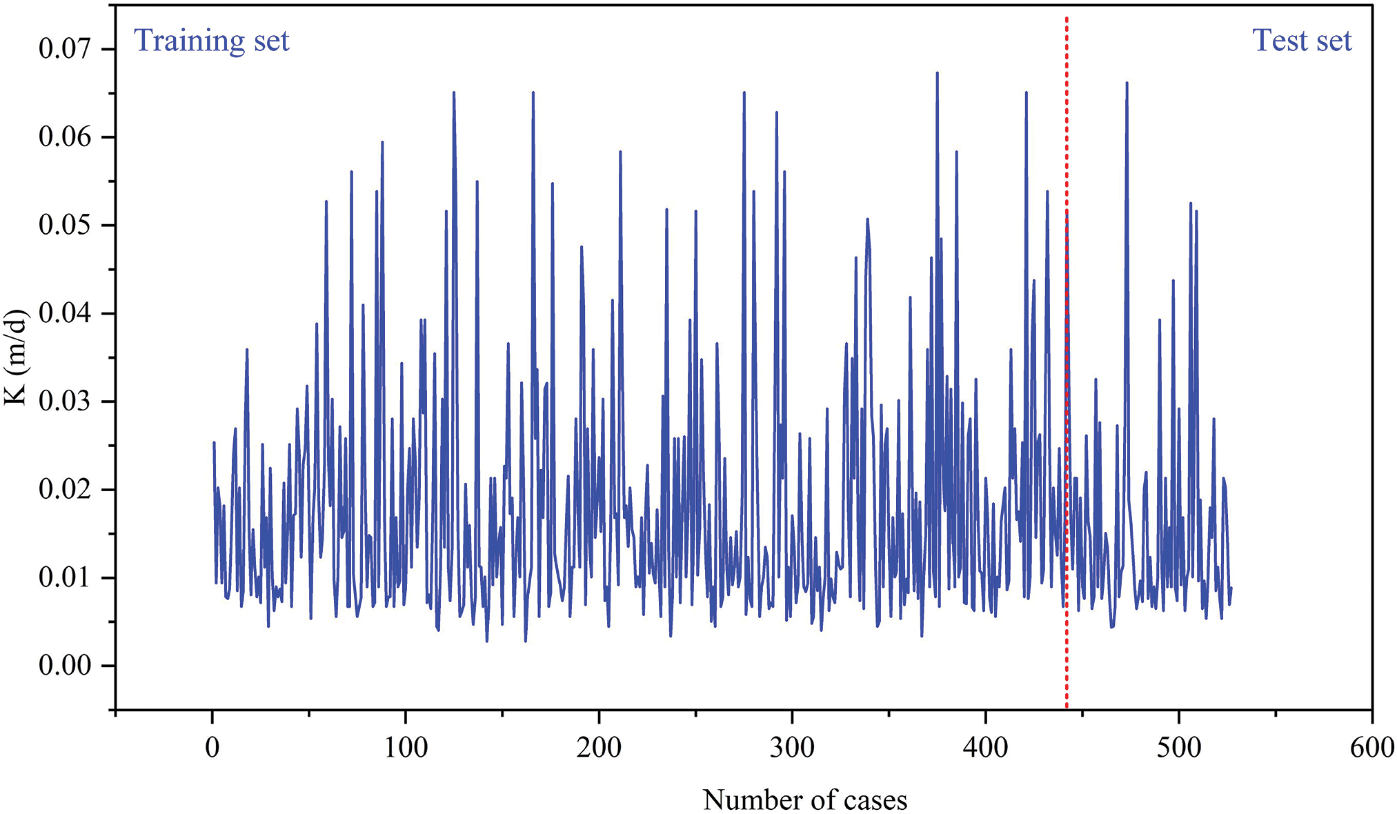
Figure 11: Output dataset
The final requirement was the predicted values of the parameter variables to verify the model’s predictive performance. Therefore, the normalized data must be converted to the original data scale during the training process, and anti-normalization must be performed.
Based on the literature [22,23] and extensive calculations (by defining a wide range of parameter spaces and observing the performance of models under different parameter combinations), the parameter settings for the ISSA–DELM method were as follows: a sparrow population size of 10 (ST = 0.6, PD = 0.7, SD = 0.1), up to 100 iterations, an activation function was sigmoid, and three hidden layers, each with ten nodes. The ISSA adds only Cauchy and OBL operators based on the SSA, and the other settings are the same as those of the SSA. Using the ISSA–DELM model to predict rock mass permeability is a minimization problem. Therefore, the best mean absolute error (MAE) in the training process was selected as the fitness function of the ISSA. The ISSA–DELM was compared to the DELM and SSA–DELM–DELM to verify the superiority of the proposed model.
The coefficient of determination (R2), mean absolute error (MAE), the root mean square error (RMSE), and relative percent deviation (RPD) were utilized to quantitatively assess the model to measure the performance of this model. The formulae are expressed as follows:
where
Generally, the smaller the value of MAE and RMSE, the lower the error with the actual value. The larger the values of
6.1 Comparison of Different Models
The results of the comparison between the measured and predicted K values are shown in Fig. 12. Because of rock mass heterogeneity and spatial variability, the results of predictive analyses using intelligent algorithms inevitably contained specific errors. Generally, if R2 is greater than 0.7, the model has good predictive ability in this field. The ISSA–DELM model had the highest fitting degree between the measured and predicted values, with an R2 of up to 0.8268, significantly higher than that of the other models. Overall, the ISSA–DELM demonstrated superior learning and training capabilities.
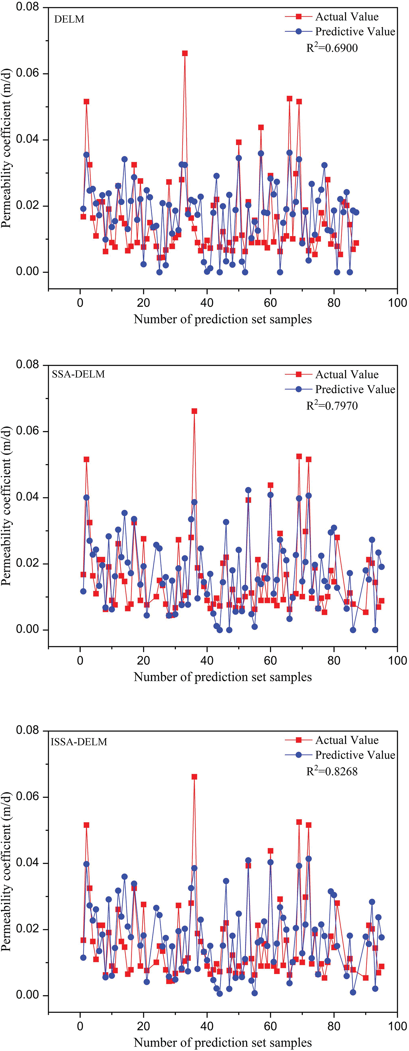
Figure 12: Comparison of different algorithms
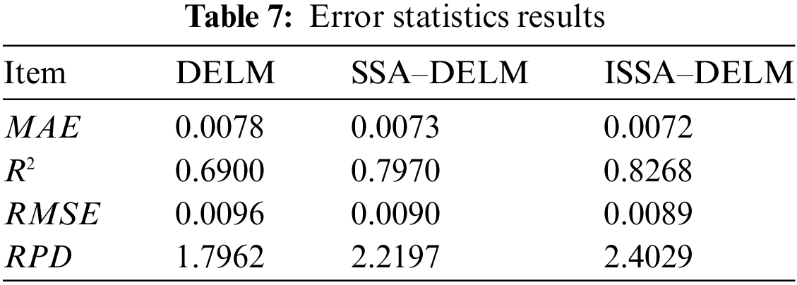
6.2 Comparison of the Results of Various Prediction Models
This study quantitatively evaluated all models using the three evaluation metrics described in Section 5.3 to fully demonstrate each model’s predictive performance. Table 7 lists the evaluation results. It shows that the MAE and RMSE values were ranked as follows: ISSA–DELM < SSA–DELM < DELM. Compared to the standalone DELM, the ISSA-DELM achieves a significant increase of approximately 16% in R2. Compared to the SSA-DELM, the ISSA-DELM performs best for all error parameters, indicating that the ISSA can obtain more appropriate parameters and further improve the optimization performance based on the SSA. In addition, the RPD of the ISSA–DELM model is greater than 2, implying that the predicted values have high reliability, indicating that they can satisfy the requirements of accurately predicting K. Considering these error assessment metrics, the ISSA–DELM model has superior performance and prediction accuracy and is appropriate for comprehensively predicting permeability coefficients in hydropower stations.
This study constructs a dataset of characteristic variables for rock mass permeability by selecting four geological indexes that are easy to obtain and have precise physical meanings on sites. Aiming at the disadvantage that the traditional SSA algorithm easily falls into local optimum at the end of training, Sine chaotic mapping, dynamic adaptive weights, Cauchy mutation, and OBL are adopted to improve the basic SSA algorithm. In addition, the improved algorithm is combined with the DELM algorithm to establish a prediction model of the rock mass permeability coefficient based on various geological indexes in the pumped storage power station project area. The main conclusions are shown below:
1. The Spearman correlation analysis method successfully identifies the main geological indexes affecting the rock mass permeability in the project area, revealing the correlation between these indexes and K. The results showed a significant negative correlation between burial depth, RQD, RID, and K, while FD indicated a moderate positive correlation with K. The proposed open-parameter model can replace or add modeling indexes based on the actual situation of different projects.
2. The diversity of solutions is expanded and enriched by adopting multiple learning strategies to improve the SSA algorithm. At the same time, the mutation and update of the optimal solution position is achieved, reducing the probability of the algorithm falling into local extremes. Compared to similar algorithms, the effectiveness and superiority of the ISSA algorithm are verified.
3. The ISSA-DELM model can make a rapid and relatively accurate prediction of the rock mass permeability in the pumped storage power station project area. The model has a good application prospect and popularization value in the analysis of seepage stability and can provide a specific reference basis for the support design of hydraulic structures.
Acknowledgement: The authors are very grateful to other professors from the School of Engineering and Technology for their theoretical support of this paper.
Funding Statement: The authors received no specific funding for this study.
Author Contributions: The authors confirm their contribution to the paper as follows: study conception and design: Yingdong Wang; analysis and interpretation of results: Chen Xing; draft manuscript preparation: Leihua Yao. All authors reviewed the results and approved the final version of the manuscript.
Availability of Data and Materials: The details of the original database are presented in the manuscript in the form of a bar chart. For further information, please contact the corresponding author.
Conflicts of Interest: The authors declare that they have no conflicts of interest to report regarding the present study.
References
1. Wang Z, Li W, Bi L, Qiao L, Liu R, Liu J. Estimation of the REV size and equivalent permeability coefficient of fractured rock masses with an emphasis on comparing the radial and unidirectional flow configurations. Rock Mech Rock Eng. 2018;51(5):1457–71. doi:10.1007/s00603-018-1422-4. [Google Scholar] [CrossRef]
2. Eid HT, Elshafie MZEB, O’Sullivan B. Simple procedure for preliminary estimation of the permeability of randomly fractured rock masses. Int J Geomech. 2024;24(3):1–11. doi:10.1061/ijgnai.Gmeng-8939. [Google Scholar] [CrossRef]
3. Wang P, Xie Y. Numerical simulation of permeability of rock-mass with multiple through filled fractures. Geotech Geol Eng. 2022;40(7):3873–87. doi:10.1007/s10706-022-02134-5. [Google Scholar] [CrossRef]
4. Zhu Z, Niu Z, Que X, Liu C, He Y, Xie X. Study on permeability characteristics of rocks with filling fractures under coupled stress and seepage fields. Water. 2020;12(10):2782. doi:10.3390/w12102782. [Google Scholar] [CrossRef]
5. Li T, Du Y, Zhu Q, Ran J, Zhang H, Xing X. Experimental study on strength properties, fracture patterns, and permeability behaviors of sandstone containing two filled fissures under triaxial compression. Bull Eng Geol Environ. 2021;80(7):5921–38. doi:10.1007/s10064-021-02286-3. [Google Scholar] [CrossRef]
6. Piscopo V, Baiocchi A, Lotti F, Ayan EA, Biler AR, Ceyhan AH, et al. Estimation of rock mass permeability using variation in hydraulic conductivity with depth: experiences in hard rocks of western Turkey. Bull Eng Geol Environ. 2018;77(4):1663–71. doi:10.1007/s10064-017-1058-8. [Google Scholar] [CrossRef]
7. Pei N, Wu Y, Su R, Li X, Wu Z, Li R, et al. Interval prediction of the permeability of granite bodies in a high-level radioactive waste disposal site using LSTM-RNNs and probability distribution. Front Earth Sci. 2022;10:1–13. doi:10.3389/feart.2022.835308. [Google Scholar] [CrossRef]
8. Winkler G, Reichl P, Sharp J. Scale dependent hydraulic investigations of faulted crystalline rocks–examples from the Eastern Alps, Austria. IAH-Selected Papers Hydrogeol. 2014;181–96. doi:10.1201/b17016-12. [Google Scholar] [CrossRef]
9. Fei T, Zhang A, Jie Y, Lin C. Inversion analysis of rock mass permeability coefficient of dam engineering based on particle swarm optimization and support vector machine: a case study. Measurement. 2023;221:113580. doi:10.1016/j.measurement.2023.113580. [Google Scholar] [CrossRef]
10. Eid HT, Elshafie MZEB, O’Sullivan B, Mahmoud A, Stollberg R. Estimating the permeability of fractured rock masses for design of construction dewatering systems. Eng Geol. 2023;323:107231. doi:10.1016/j.enggeo.2023.107231. [Google Scholar] [CrossRef]
11. Gui Y, Xia C, Ding W, Qian X, Du S. Modelling shear behaviour of joint based on joint surface degradation during shearing. Rock Mech Rock Eng. 2019;52(1):107–31. doi:10.1007/s00603-018-1581-3. [Google Scholar] [CrossRef]
12. Wu Q, Yan B, Zhang C, Wang L, Ning G, Yu B. Displacement prediction of tunnel surrounding rock: a comparison of support vector machine and artificial neural network. Math Probl Eng. 2014;2014(1):351496. doi:10.1155/2014/351496. [Google Scholar] [CrossRef]
13. Upadhya A, Thakur MS, Sihag P, Kumar R, Kumar S, Afeeza A, et al. Modelling and prediction of binder content using latest intelligent machine learning algorithms in carbon fiber reinforced asphalt concrete. Alex Eng J. 2022;65:131–49. doi:10.1016/j.aej.2022.09.055. [Google Scholar] [CrossRef]
14. Song C, Yao L. Application of artificial intelligence based on synchrosqueezed wavelet transform and improved deep extreme learning machine in water quality prediction. Environ Sci Pollut Res. 2022;29(25):38066–82. doi:10.1007/s11356-022-18757-3. [Google Scholar] [PubMed] [CrossRef]
15. Tang J, Deng C, Huang GB. Extreme learning machine for multilayer perceptron. IEEE Trans Neural Netw Learn Syst. 2016;27(4):809–21. doi:10.1109/tnnls.2015.2424995. [Google Scholar] [PubMed] [CrossRef]
16. Deng C, Huang G, Xu J, Tang J. Extreme learning machines: new trends and applications. Sci China Inf Sci. 2015;58(2):1–16. doi:10.1007/s11432-014-5269-3. [Google Scholar] [CrossRef]
17. An G, Chen L, Tan J, Jiang Z, Li Z, Sun H. Ultra-short-term wind power prediction based on PVMD-ESMA-DELM. Energy Rep. 2022;8:8574–88. doi:10.1016/j.egyr.2022.06.079. [Google Scholar] [CrossRef]
18. Lv M, Zhao J, Cao S, Tang Z. NOx emission prediction based on SSA-DELM via CFD and DCS data fusion. Int J Heat Technol. 2022;40(6):1514–21. doi:10.18280/ijht.400621. [Google Scholar] [CrossRef]
19. Chen Z, Guo Y, Guo C. Prediction of GHG emissions from Chengdu Metro in the construction stage based on WOA-DELM. Tunn Undergr Sp Tech. 2023;139:105235. doi:10.1016/j.tust.2023.105235. [Google Scholar] [CrossRef]
20. Andi T, Huan Z, Tong H, Lei X. A chaos sparrow search algorithm with logarithmic spiral and adaptive step for engineering problems. Comput Model Eng Sci. 2022;130(1):331–64. doi:10.32604/cmes.2021.017310. [Google Scholar] [CrossRef]
21. Xue J, Shen B. A novel swarm intelligence optimization approach: sparrow search algorithm. Syst Sci Control Eng. 2020;8(1):22–34. doi:10.1080/21642583.2019.1708830. [Google Scholar] [CrossRef]
22. Song C, Yao L, Hua C, Ni Q. A novel hybrid model for water quality prediction based on synchrosqueezed wavelet transform technique and improved long short-term memory. J Hydrol. 2021;603:126879. doi:10.1016/j.jhydrol.2021.126879. [Google Scholar] [CrossRef]
23. Mao Q, Zhang Q. Improved sparrow algorithm combining cauchy mutation and opposition-based learning. J Frontiers Comput Sci Technol. 2021;15(6):1155–64 (In Chinese). doi:10.3778/j.issn.1673-9418.2010032. [Google Scholar] [CrossRef]
24. Qiao L, Jia Z, Cui Y, Xiao K, Su H. Shear sonic prediction based on DELM optimized by improved sparrow search algorithm. Appl Sci. 2022;12(8260):8260. doi:10.3390/app12168260. [Google Scholar] [CrossRef]
25. Liu C, Niu P, Li G, Ma Y, Zhang W, Chen K. Enhanced shuffled frog-leaping algorithm for solving numerical function optimization problems. J Intell Manuf. 2018;29(5):1133–53. doi:10.1007/s10845-015-1164-z. [Google Scholar] [CrossRef]
26. Yang HD, E JQ. An adaptive chaos immune optimization algorithm with mutative scale and its application. Control Theory Appl. 2009;26(10):1069–74. [Google Scholar]
27. Liu J, Yuan M, Zuo F. Global search-oriented adaptive leader salp swarm algorithm. Control Decis. 2021;36(9):2152–60 (In Chinese). doi:10.13195/j.kzyjc.2020.0090. [Google Scholar] [CrossRef]
28. Tizhoosh HR. Opposition-based learning: a new scheme for machine intelligence. In: International Conference on Computational Intelligence for Modeling, Control and Automation and International Conference on lntelligent Agents, Web Technologies and Internet Commerce; 2005 Nov 28–30; Vienna, Austria. [Google Scholar]
29. He Q, Lin J, Xu H. Hybrid Cauchy mutation and uniform distribution of grasshopper optimization algorithm. Control Decis. 2021;36(7):1558–68 (In Chinese). doi:10.13195/j.kzyjc.2019.1609. [Google Scholar] [CrossRef]
30. Stober I, Bucher K. Hydraulic properties of the crystalline basement. Hydrogeol J. 2007;15(2):213–24. doi:10.1007/s10040-006-0094-4. [Google Scholar] [CrossRef]
31. Zhang L. Aspects of rock permeability. Front Struct Civil Eng. 2013;7(2):102–16. doi:10.1007/s11709-013-0201-2. [Google Scholar] [CrossRef]
32. Achtziger-Zupancic P, Loew S, Mariethoz G. A new global database to improve predictions of permeability distribution in crystalline rocks at site scale. J Geophys Res-Solid Earth. 2017;122(5):3513–39. doi:10.1002/2017jb014106. [Google Scholar] [CrossRef]
33. Wei ZQ, Egger P, Descoeudres F. Permeability predictions for jointed rock masses. Int J Rock Mech Min Sci Geomech Abstr. 1995;32(3):251–61. doi:10.1016/0148-9062(94)00034-z. [Google Scholar] [CrossRef]
34. Qureshi MU, Khan KM, Bessaih N, Al-Mawali K, Al-Sadrani K. An empirical relationship between in-situ permeability and RQD of discontinuous sedimentary rocks. Electron J Geotech Eng. 2014;19:3032. [Google Scholar]
35. El-Naqa A. The hydraulic conductivity of the fractures intersecting Cambrian sandstone rock masses, central Jordan. Environ Geol. 2001;40(8):973–82. doi:10.1007/s002540100266. [Google Scholar] [CrossRef]
36. Öge IF. Assessing rock mass permeability using discontinuity properties. Procedia Eng. 2017;191:638–45. doi:10.1016/j.proeng.2017.05.373. [Google Scholar] [CrossRef]
37. Jiang X, Wan L, Wang X, Wu X, Zhang X. Estimation of rock mass deformation modulus using variations in transmissivity and RQD with depth. Rock Soil Mech. 2009;46(8):1370–7 (In Chinese). doi:10.1016/j.ijrmms.2009.05.004. [Google Scholar] [CrossRef]
38. Kun S, Echuan Y, Gang C. Hydraulic conductivity estimation of rock mass in water sealed underground storage caverns. Chinese J Rock Mech Eng. 2014;33(3):575–80 (In Chinese). doi:10.13722/j.cnki.jrme.2014.03.016. [Google Scholar] [CrossRef]
Cite This Article
 Copyright © 2024 The Author(s). Published by Tech Science Press.
This work is licensed under a Creative Commons Attribution 4.0 International License , which permits unrestricted use, distribution, and reproduction in any medium, provided the original work is properly cited.
 Downloads
 Citation Tools