Bayesian and Non-Bayesian Analysis for the Sine Generalized Linear Exponential Model under Progressively Censored Data

1  Introduction

In various practical fields like medicine, engineering, and finance, among others, it is essential to model and analyze data related to the lifespan of objects or processes. Various lifetime distributions have been applied to describe such data. For example, the exponential and Rayleigh distributions and their variations. Each distribution possesses unique features determined by the behavior of the failure rate function, which can either steadily decrease or increase, remain constant, exhibit non-monotonic patterns, have a bathtub-shaped curve, or even follow an unimodal trend. In [1], Sarhan et al. proposed the generalized linear failure rate (GLFR) distribution which has another name the GLE distribution. It has a decreasing or unimodal probability density function (PDF) and its HRF can be increasing, decreasing, and bathtub-shaped. The GLE distribution has many applications in applied statistics and reliability analysis. The GLFR distribution is very flexible and has more special cases, as linear failure rate (linear exponential) (LFR), generalized exponential, generalized Rayleigh, exponential and Rayleigh a very well-known distribution for modeling lifetime data in reliability and medical studies. Lifetime data is frequently analyzed using the exponential, Rayleigh, linear failure rate, or exponentiated exponential distributions. It is well known that an exponential distribution can only have a constant HRF, whereas Rayleigh, linear failure rate, and generalized exponential distributions can only have monotone HRFs (increasing in the case of Rayleigh or LFR and increasing/decreasing in the case of the generalized exponential distribution). However, in practice, non-monotonic functions like bathtub-shaped HRFs must also be considered. However, the GLE distribution has a bathtub-shaped HRF and generalizes several well-known distributions, including the traditional LFR distribution. The previous elements motivate us to introduce a new extension of the GLE distribution. The cumulative distribution function (CDF) and the PDF for GLE are as follows:

H(x;α,θ,λ)=(1−e−αx−θ2x2)λ,x>0,(1)

and

h(x;α,θ,λ)=λ(α+θx)e−(αx+θ2x2)(1−e−αx−θ2x2)λ−1,(2)

respectively, where λ>0 is a shape parameter, α>0 and θ>0 are scale parameters. Many researchers constructed generalizations of the GLE distribution. For instance, various univariate extensions of the GLFR distribution have been introduced, including the generalized linear exponential (GLE) [2], beta linear failure rate [3], exponentiated GLFR [4], generalized exponential LFR [5], odd generalized exponential GLFR [6], inverted GLFR [7], Marshall-Olkin extended GLFR [8], truncated Cauchy power LFR [9] and modified beta GLFR [10] distributions.

Over recent years, numerous methods for augmenting parameters in distributions have been put forth and examined. These expanded distributions offer versatility in specific applications, including but not limited to economics, engineering, biological studies, and environmental sciences. Some well-known families are the Marshall-Olkin-G by [11], the beta-G by [12], the Kumaraswamy-G by [13], the logistic-G by [14], exponentiated generalized-G by [15], the Weibull-G by [16], the logistic-X family by [17], generalized inverted kumaraswamy by [18], marshall-olkin odd Burr III-G family by [19], type II exponentiated half logistic generated family by [20], odd generalized N-H generated family by [21], new truncated muth generated family by [22], exponentiated generalized Weibull exponential by [23], and new inverse Rayleigh distribution by [24].

Recently, there has been a growing focus on developing families of distributions based on trigonometric functions. These families offer a balance between simplicity in their definitions, enabling a clear understanding of their mathematical properties, and a high degree of applicability for modeling various real-world datasets. This balance is achieved through the effective utilization of flexible trigonometric functions. As far as we are aware, the sine-G family of distributions is one of the earliest examples of such trigonometric distribution families. In [25], Kumar et al. introduced a novel approach for generating new probability distributions by modifying trigonometric functions. They modified the sine function to create a unique statistical distribution known as the sine-G family, with the CDF and PDF defined as follows:

FS(x;κ)=sin⁡(π2H(x;κ)),x∈R,(3)

fS(x;κ)=π2h(x;κ)cos⁡(π2H(x;κ)),(4)

respectively. The HRF is given by

ξS(x;κ)=π2h(x;κ)tan⁡(π4(1+H(x;κ))),(5)

where H(x;κ) and h(x;κ) are the CDF and PDF of a certain continuous distribution with parameters vector denoted by κ=(α,θ,λ). This family has many advantages like, it is simple form, the two cumulative functions F(x;κ) and H(x;κ) have the same number of parameters; there is no additional parameter, avoiding any problem of over-parametrization, In addition to, F(x;κ) has the ability to increase the flexibility of H(x;κ), providing new flexible models. These distributions are linked to a predefined reference distribution, a choice made by the practitioner according to the specific study’s context. It has been confirmed that the S-G family (i) provides an appealing alternative to the reference family, as it satisfies the inequality H(x;κ)≤FS(x;κ) for any x∈R, (ii) maintains an acceptable level of mathematical complexity without introducing additional parameters, and (iii) offers the flexibility to construct diverse statistical models capable of handling data with varying characteristics.

Other trigonometric families of distributions have been developed. See, for instance, beta trigonometric distribution by [26], hyperbolic cosine-F family [27], odd hyperbolic cosine family of lifetime distributions by [28], odd hyperbolic cosine exponential-exponential distribution by [29], transmuted arcsine distribution by [26], the arcsine exponentiated-X family by [30].

The failure of components and units, which make up the majority of operational systems in the fields of industrial and mechanical engineering, has been extensively studied by statisticians. Their research focuses on tracking the functioning units until they fail, recording their lifespans, using statistical inference methods to analyze the data gathered, and then calculating the reliability and hazard functions for the entire system using the data gathered. However, some experimental units are pricey and very reliable; therefore, in this case, the number of experimental units and the length of the lifetime experiment of these units must be reduced. The progressively Type-II censoring strategy satisfies the lifespan experiment’s requirements for good estimators while preventing certain experimental units from failing.

The main objectives of this study are to contribute to the statistical literature and address some issues about the failure of units and components for various applications of the extension model of the trigonometric family. The following reasons are sufficient justification for doing so:

•   Introducing the sine generalized linear exponential distribution as a novel three-parameter model based on the sine-G family of distributions.

•   The PDF can exhibit several features, such as being unimodal, declining, right-skewed, or heavy-tailed. Similarly, the HRF might display growing, J-shaped. These properties are desired in a range of applications, such as survival analysis, reliability, and uncertainty modeling.

•   There is a closed-form expression for the equivalent quantile.

•   The new suggested model is very flexible and it has five sub-models.

•   It is possible to compute several statistical features, including the quantiles, Bowley’s skewness, Moor’s kurtosis, moments, moment generating function, incomplete moments, conditional moments, Lorenz and Bonferroni curves, residual life and inverted residual life functions, and so on.

•   Using progressively Type-II censoring schemes to prevent certain experimental units from failing.

•   The parameters of the SGLE distribution can be estimated utilizing by Bayesian and non-Bayesian estimation methods.

•   For illustrative purposes, this study examines SGLE distribution distinct datasets in the actual world. We demonstrate, by highlighting its functionalities, that the SGLE distribution may serve as a more viable alternative to formidable competitors.

This article’s remaining sections are organized as follows. The sine generalized linear exponential distribution and its sub-models are represented in Section 2. Section 3 introduces a linear representation of the SGLE density function. Section 4 provides information on the statistical characteristics of the SGLE distribution, such as quantiles, Bowley’s skewness, Moor’s kurtosis, moments, moment generating function, incomplete moments, conditional moments, Lorenz and Bonferroni curves, residual life and inverted residual life functions. In Section 5, the progressively Type-II censoring scheme is carried out. In Section 6, the model parameters’ Bayesian and non-Bayesian inference is carried out. In Section 7, two real datasets show the applicability and flexibility of the SGLE distribution. Section 8 delves into the results of the simulation. Furthermore, the conclusion is presented in Section 9, which is located at the end of the paper.

2  Sine Generalized Linear Exponential Model

In this section, we construct a new flexible model called the sine generalized linear exponential model by inserting (1) into (3), we obtain the CDF as follows:

FSGLE(x;κ)=sin⁡[π2(1−e−αx−θ2x2)λ],x>0,(6)

and the corresponding PDF is

fSGLE(x;κ)=π2λ(α+θx)e−(αx+θ2x2)(1−e−αx−θ2x2)λ−1cos⁡[π2(1−e−αx−θ2x2)λ],(7)

where κ=(α,θ,λ). The survival function and HRF for the SGLE are, respectively, given by

F¯SGLE(x;κ)=1−sin⁡[π2(1−e−αx−θ2x2)λ],(8)

ξSGLE(x;κ)=πλ2(α+θx)e−(αx+θ2x2)(1−e−αx−θ2x2)λ−1×tan⁡[π4(1+(1−e−αx−θ2x2)λ].(9)

Fig. 1 discussed density and hazard rate for the SGLE distribution with different values of parameters.

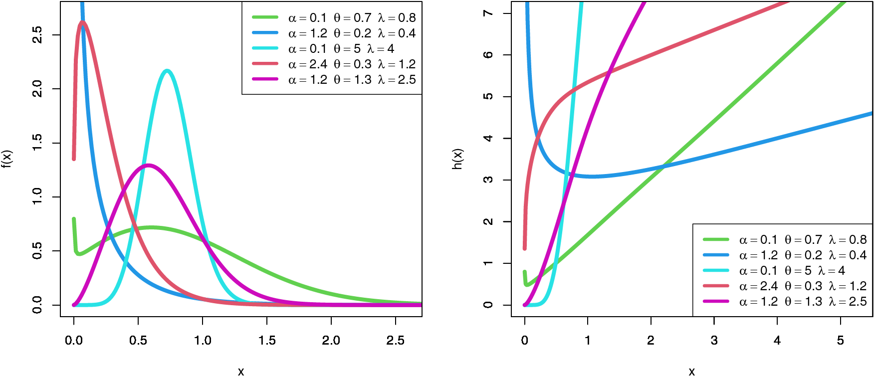
Figure 1: Density and hazard rate for the SGLE distribution

2.1 Some Special Models of the SGLE Model

The SGLE model contains five sub-models:

1.   At λ = 1 the SGLE model reduces to the sine LE model.

2.   At θ = 0 the SGLE model reduces to the sine generalized exponential model.

3.   At α = 0 the SGLE model reduces to the sine generalized Rayleigh model.

4.   At λ = 1, θ = 0 the SGLE model reduces to the sine exponential model.

5.   At λ = 1, α = 0 the SGLE model reduces to the sine Rayleigh model.

3  Linear Representation of the SGLE Density Function

In this section, we derived the density expansion of the SGLE distribution. Using the Taylor series expansion of the cosine function,

cos⁡[π2G(x)]=∑i=0∞(−1)i(2i)!(π2G(x))2i,

we have

cos⁡[π2(1−e−αx−θ2x2)λ]=∑i=0∞(−1)i(2i)!(π2)2i(1−e−αx−θ2x2)2λi,(10)

fSGLE(x;κ)=λ∑i=0∞(−1)i(2i)!(π2)2i+1(α+θx)e−(αx+θ2x2)(1−e−αx−θ2x2)λ(2i+1)−1.(11)

But

(1−e−αx−θ2x2)λ(2i+1)−1=∑j=0∞(−1)j(λ(2i+1)−1j)e−j(αx+θ2x2),(12)

applying (12) in (11), we obtain

fSGLE(x;κ)=λ∑i,j=0∞(−1)i+j(2i)!(π2)2i(λ(2i+1)−1j)(α+θx)e−(j+1)(αx+θ2x2).(13)

Expanding e−(j+1)θ2x2 in power series as

e−(j+1)θ2x2=∑k=0∞(−1)k(j+1)kk!(θ2)kx2k,(14)

inserting (14) in (13) the SGLE density function can be written as

fSGLE(x;κ)=∑i,j,k=0∞ωi,j,k (αx2k+θx2k+1)e−(j+1)αx,(15)

ωi,j,k=λ∑i,j=0∞(−1)i+j+k(j+1)k(2i)!k!(π2)2i+1(θ2)k(λ(2i+1)−1j).

4  Statistical Properties

In this section, we studied some important mathematical and statistical properties of the SGLE distribution, specifically quantile function, ordinary moments, incomplete moments, Lorenz and Bonferroni curves, and moments of the residual life and reversed residual lives.

4.1 Quantile Function

Quantile functions find utility in theoretical, statistical, and Monte Carlo scenarios. In Monte Carlo simulations, these functions are utilized to generate simulated random variables for both traditional and contemporary continuous distributions. To derive the quantile function Q(u) for the SGLE distribution, represented as x=Q(u), we can obtain it by reversing the process described in Eq. (6) as follows:

Q(u;κ)=FSGLE−1(u;κ)=−α+α2−2θln⁡[1−(2πarcsin⁡(u))1λ]θ,u∈(0,1),(16)

The median is given by

Median=−α+α2−2θln⁡[1−(2πarcsin⁡(0.5))1λ]θ.

One of the initial proposals for a skewness measure is the Bowley skewness, introduced by Kenney and Keeping in 1962, and it is defined as follows:

SK=Q(34)+Q(14)−2Q(12)Q(34)−Q(14).

Conversely, the Moors kurtosis, as introduced by Moors in 1988 and calculated using quantiles, is expressed as

KU=Q(78)−Q(58)+Q(38)−Q(18)Q(68)−Q(28).

In this context, Q(.) denotes the quantile function. The metrics SK and KU exhibit reduced sensitivity to extreme data points, and they are applicable to distributions that may not possess moments. In the case of symmetric unimodal distributions, a positive kurtosis value suggests that the distribution has heavier tails and is more peaked compared to a normal distribution, while a negative kurtosis value indicates lighter tails and a flatter shape. Fig. 2 discusses SK and KT for the SGLE distribution with different values of parameters.

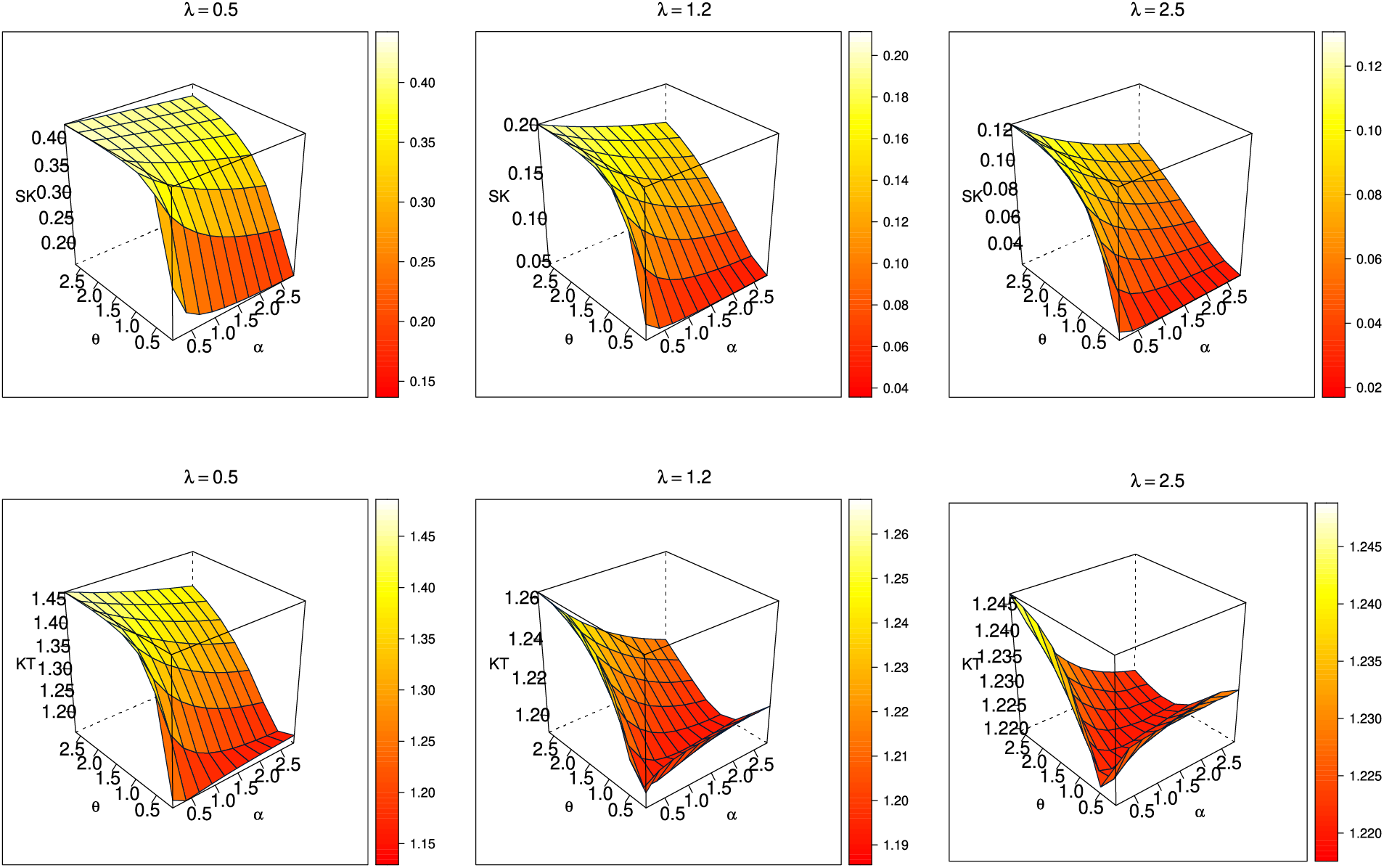
Figure 2: Bowley skewness and Moors kurtosis for the SGLE distribution

4.2 Moments and Moment Generating Functions

In this particular section, we will establish the formulas for both the typical and moment-generating functions of the SGLE distribution. These moment calculations for various orders are essential for estimating the device’s expected lifespan, as well as assessing the spread, skewness, and kurtosis of data sets encountered in reliability-related situations.

4.2.1 Moments

The rth moment of the SGLE distribution can be derived using Eq. (7).

μr/=E(Xr)=∫0∞xrfSGLE(x;κ)dx=∑i,j,k=0∞ωi,j,k ∫0∞(αx2k+r+θx2k+r+1)e−(j+1)αxdx.

After a series of transformations, which involve substituting a new variable z=(j+1)αx and introducing the gamma function, we arrive at the following result:

μr/=∑i,j,k=0∞ωi,j,k(α+θ(2k+r+1)α(j+1))Γ(2k+r+1)[α(j+1)]2k+r+1.(17)

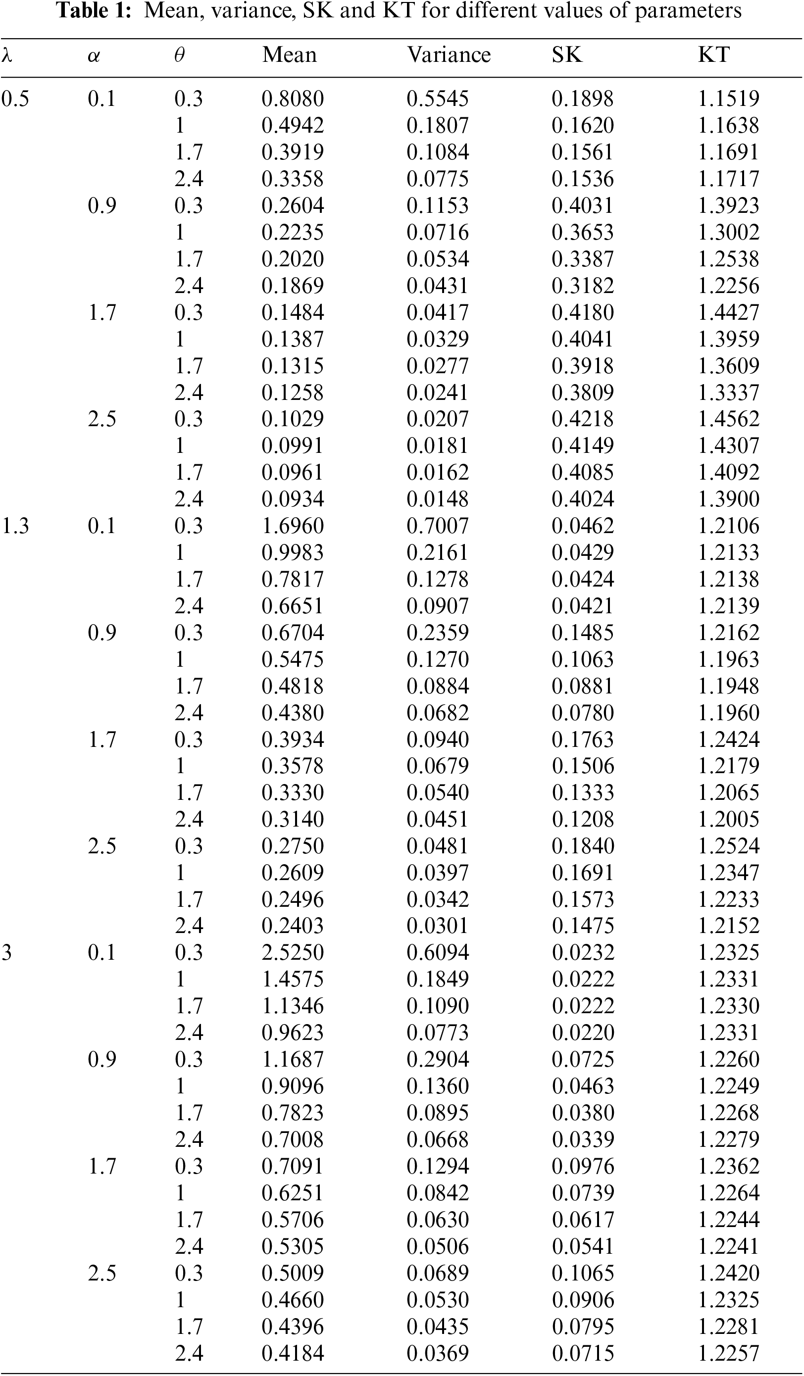
Table 1 shows some numerical values of moments for the SGLE distribution.

4.2.2 Moment Generating Function

The moment-generating function of the SGLE distribution is

M(t)=E(etX)=∫0∞etxfSGLE(x;κ)dx=∑i,j,k=0∞ωi,j,k ∫0∞(αx2k+θx2k+1)e−[(j+1)α−t]xdx=∑i,j,k=0∞ωi,j,k(α+θ(2k+1)α(j+1)−t)Γ(2k+1)[α(j+1)−t]2k+1.(18)

4.3 Incomplete Moments

The sth incomplete moment of the SGLE distribution is given by

ξs(t)=E(xs∣X<t)=∫0txsfSGLE(x;κ)dx=∑i,j,k=0∞ωi,j,k ∫0t(αx2k+s+θx2k+s+1)e−(j+1)αxdx=∑i,j,k=0∞ωi,j,k[αγ(2k+s+1,(j+1)αt)[(j+1)α]2k+s+1+θγ(2(k+1)+s,(j+1)αt)[(j+1)α]2(k+1)+s],(19)

where γ(n,x)=∫0xtn−1e−tdt denotes the lower incomplete gamma function.

4.4 Conditional Moments

The conditional moment of the SGLE distribution can be written as

Ωs(t)=E(xs∣X>t)=1F¯(t)ψs(t)

where

ψs(t)=∫t∞xsfSGLE(x;κ)dx=∑i,j,k=0∞ωi,j,k ∫t∞(αx2k+s+θx2k+s+1)e−(j+1)αxdx=∑i,j,k=0∞ωi,j,k[αΓ(2k+s+1,(j+1)αt)[(j+1)α]2k+s+1+θΓ(2(k+1)+s,(j+1)αt)[(j+1)α]2(k+1)+s],(20)

where Γ(n,x)=∫x∞tn−1e−tdt denotes the upper incomplete gamma function.

4.5 Lorenz and Bonferroni Curves

The Lorenz curve was first introduced by Lorenz in the year 1905, and the Bonferroni curve. These curves have found applications in various fields, including economics, where they are used to analyze income distribution and poverty. Additionally, they serve as tools for quantifying the inequality within the distribution of a variable and apply to a wide range of disciplines, such as reliability, demography, medicine, and insurance. For a positive random variable X, both the Lorenz and Bonferroni curves, at a specified probability p, can be expressed as follows:

L(p)=1μ∫0qxf(x)dx=1μ∑i,j,k=0∞ωi,j,k[αγ(2(k+1),(j+1)αq)[(j+1)α]2(k+1)+θγ(2(k+1)+1,(j+1)αq)[(j+1)α]2(k+1)+1],(21)

and

B(p)=1μp∫0qxf(x)dx=1μp∑i,j,k=0∞ωi,j,k[αγ(2(k+1),(j+1)αq)[(j+1)α]2(k+1)+θγ(2(k+1)+1,(j+1)αq)[(j+1)α]2(k+1)+1],(22)

respectively, where μ=E(X), and q=Q(p) is the quantile function of X at p.

4.6 Residual Life and Reversed Residual Life Functions

Assume that a component remains operational until time t≥0. The residual life is the duration from time t until the point of failure, and it is described by the conditional random variable denoted as X−t|X>t. The rth-order moment of the residual life is

μr(t)=E((X−t)r∣X>t)=1F¯(t)∫t∞(x−t)r f(x)dx,r≥1.

For SGLE distribution, we get

μr(t)=1F¯(t)∑i,j,k=0∞∑h=0rωi,j,k(rh)(−t)r−h∫t∞xrfSGLE(x;κ)dx=1F¯(t)∑i,j,k=0∞∑h=0rωi,j,k(rh)(−t)r−h[αΓ(2k+r+1,(j+1)αt)[(j+1)α]2k+r+1+θΓ(2(k+1)+r,(j+1)αt)[(j+1)α]2(k+1)+r].(23)

The average remaining lifespan (also known as the life expectancy at time t) signifies the anticipated additional life duration for a component or device that is still functioning at age t. To calculate the mean residual life (MRL) for the SGLE distribution, you can set r=1 in Eq. (23), which is defined as

μ(t)=E(Xt)=E(X∣X>t).

In the realm of reliability theory, the extra time a component can continue operating after it has already failed by time t is referred to as the reversed residual life function (RRL). It represents the duration of time the component remains inactive. The conditional random variable X(t)=t−X|X<t denotes the time that has passed since the failure of X, given that it failed at or before time t. The rth order moment of the reversed residual life, also known as the inactivity time, can be calculated using a commonly known formula.

mr(t)=E((t−X)r∣X≤t)=1F(t)∫0t(t−x)rf (x)dx,r≥1=1F(t)∑i,j,k=0∞∑h=0rωi,j,k(rh)(−t)r−h∫0txrfSGLE(x;κ)dx=1F(t)∑i,j,k=0∞∑h=0rωi,j,k(rh)(−t)r−h[αγ(2k+r+1,(j+1)αt)[(j+1)α]2k+r+1+θγ(2(k+1)+r,(j+1)αt)[(j+1)α]2(k+1)+r].

5  Progressively Type-II Censoring Schemes

Progressively censored samples are those that are removed from further analysis at different phases of an experiment, while not all of the remaining specimens are. Sample specimens that are still present after each censorship stage are kept under observation until they fail or until the next censoring stage.

Under progressively Type-II censored samples: Firstly, the experimenter adds n independent, identical units to the measure of life. Secondly, the experimenter determines m observation of the censored sample. Thirdly, the experimenter chooses optimal scheme R by the experience of the experimenter but the following constrains must be met as: Ri≥0; n−m+∑i=1mRi=0. The remaining n−1 surviving units get R1 units randomly removed from them after the first failure occurs, let us say at time x1:m:n. The remaining n−R1−2 surviving units get R2 units randomly removed from them when the second failure occurs at time x2:m:n. When the mth failure occurs at time xm:m:n, the experiment is over, and the Rm=n−m−∑i=1m−1Ri surviving units are taken out of the test. The progressive Type-II censoring method is denoted by R=(R1,R2,…,Rm). progressive Type-II censoring, with a predetermined R censoring scheme.

Assume that n independent units are put through a life test with the associated failure times of x1:m:n<x2:m:n<⋯<xm:m:n, and m, respectively. Additionally, assume that the progressive Type-II censoring scheme is R1,R2,…,Rm and that the pre-fixed number of failures to be seen is m. The failure times that have been m entirely observed will be shown as xi:m:n;i=1,2,…,m. The likelihood function is then as follows:

L(x;κ)=C∏i=1mf(xi:m:n;κ)[1−F(xi:m:n;κ)]Ri,(24)

where C may be a constant defined as C=n(n−R1−1)⋯(n−∑i=1m−1(Ri+1)) (see [31] for details) and see Fig. 3.

Figure 3: A diagram showing Type-II progressive censorship

Based on the SGLE distribution by Eqs. (6), (7) and (24), the likelihood function of the SGLE based on progressive Type-II censored sample is then as follows:

L(x;κ)=(π2)nλne−∑i=1m(αxi:m:n+θ2x2)∏i=1m(α+θxi:m:n)(1−e−αxi:m:n−θ2xi:m:n2)λ−1×∏i=1mcos⁡[π2(1−e−αxi:m:n−θ2xi:m:n2)λ].(25)

Based on Eq. (25) and Fig. 3, we note that there is more than one special case, such as the following:

•   Complete sample when m=n and Ri=0;i=1,…,m.

•   Type-II censored sample when m<n and Rm=n−m and Ri=0;i=1,…,m−1.

More information on the increasingly progressive censored samples may be found in Balakrishnan et al. [32] and Balakrishnan et al. [31]. Aggarwala et al. [33] have discussed the differences in the situation of progressive Type-II censoring where lifespan distributions are Weibull, log-normal, and exponential. For more information and examples, see [34–37].

6  Inference and Estimation Methods

In this section, Bayesian and non-Bayesian inference have been discussed for parameters of SGLE distribution.

6.1 Maximum Likelihood Estimation

The maximum likelihood estimates (MLEs) possess favorable characteristics and find utility in constructing confidence intervals, regions, and test statistics. We calculate the MLEs for the parameters of the SGLE distribution using complete samples exclusively, see [38,39]. Consider a random sample of size n, denoted as x1,...,xn, drawn from the SGLE distribution as defined in Eq. (7). Let Un(κ)=(∂Ln∂α,∂Ln∂θ,∂Ln∂λ)T be q×1 vector of parameters. The log-likelihood function is given by

Ln=nlog⁡(π2)+nlog⁡(λ)+∑i=1nlog⁡(α+θxi:m:n)−α∑i=1nxi:m:n−θ2∑i=1nxi:m:n2+(λ−1)∑i=1nlog⁡(1−e−αxi:m:n−θ2xi:m:n2)+∑i=1nlog⁡cos⁡[π2(1−e−αxi:m:n−θ2xi:m:n2)λ]+∑i=1mRilog⁡{1−sin⁡[π2(1−e−αxi:m:n−θ2xi:m:n2)λ]}.(26)

The log-likelihood can be maximized through direct utilization of the SAS program or R-language, or by solving the nonlinear likelihood equations derived from differentiating (26).

∂Ln∂α=∑i=1n1(α+θxi:m:n)−∑i=1nxi:m:n+(λ−1)∑i=1nxi:m:ne−αxi:m:n−θ2xi:m:n21−e−αxi:m:n−θ2xi:m:n2−π2∑i=1nxi:m:ne−αxi:m:n−θ2xi:m:n2tan⁡[π2(1−e−αxi:m:n−θ2xi:m:n2)λ]−λπ2∑i=1mRixi:m:ne−αxi:m:n−θ2xi:m:n2(1−e−αxi:m:n−θ2xi:m:n2)λ−1cos⁡[π2(1−e−αxi:m:n−θ2xi:m:n2)λ]1−sin⁡[π2(1−e−αxi:m:n−θ2xi:m:n2)λ],(27)

∂Ln∂θ=∑i=1nxi:m:n(α+θxi:m:n)−12∑i=1nxi:m:n2+(λ−1)∑i=1nxi:m:n22e−αxi:m:n−θ2xi:m:n21−e−αxi:m:n−θ2xi:m:n2−π4∑i=1nxi:m:n2e−αxi:m:n−θ2xi:m:n2tan⁡[π2(1−e−αxi:m:n−θ2xi:m:n2)λ]−λπ2∑i=1mRixi:m:n22e−αxi:m:n−θ2xi:m:n2(1−e−αxi:m:n−θ2xi:m:n2)λ−1cos⁡[π2(1−e−αxi:m:n−θ2xi:m:n2)λ]1−sin⁡[π2(1−e−αxi:m:n−θ2xi:m:n2)λ],(28)

∂Ln∂λ=nλ+∑i=1nlog⁡(1−e−αxi:m:n−θ2xi:m:n2)−π2∑i=1n(1−e−αxi:m:n−θ2xi:m:n2)λ×log⁡(1−e−αxi:m:n−θ2xi:m:n2)tan⁡[π2(1−e−αxi:m:n−θ2xi:m:n2)λ]+π2∑i=1mRilog⁡(1−e−αxi:m:n−θ2xi:m:n2)(1−e−αxi:m:n−θ2xi:m:n2)λcos⁡[π2(1−e−αxi:m:n−θ2xi:m:n2)λ]1−sin⁡[π2(1−e−αxi:m:n−θ2xi:m:n2)λ].(29)

The maximum likelihood estimation (MLE) of parameters is obtained by setting ∂Ln∂α=∂Ln∂θ=∂Ln∂λ=0 and solving these equations simultaneously to get the MLE(κ^). These equations cannot be solved analytically, and statistical software can be used to solve them numerically via iterative methods. Since the closed-form solutions to Eqs. (27)–(29) do not exist based on progressive Type-II censored samples, the Newton-Raphson (NR) iteration method is used to obtain the estimations. In the reference [40], the algorithm is described with the (maxLik) package which implements the NR iteration of maximization.

It is standard that under some regularity conditions, α^, θ^ and λ^ are approximately distributed as multivariate normal with mean α,θ and λ covariance matrix I−1(α,θ,λ). Then, the 100(1−γ)% two sided confidence interval of α,θ and λ, can be given by

α^±Zγ2Var(α^), & θ^±Zγ2Var(θ^), & λ^±Zγ2Var(λ^),(30)

where Zγ2 is that the percentile of the standard normal distribution with right-tail probability γ2.

6.2 Bayesian Estimation Method

In this subsection, we establish Bayesian estimates that treat the parameter uncertainty as being represented by a joint prior distribution that was created prior to the failure data being gathered. Because it allows for the inclusion of prior knowledge in the study, the Bayesian technique is very helpful in reliability analysis. Based on the square error loss function (SELF), Bayesian estimates of the unknown parameters α,θ, and λ are derived. The parameters α,θ, and λ are assumed to be independent and to follow the following gamma prior distributions:

{π1(α)∝αq1−1e−w1α,α>0,π2(θ)∝θq2−1e−w2θ,θ>0,π3(λ)∝λq3−1e−w3λ,λ>0,(31)

where it is assumed that all of the hyper-parameters qi and wi have non-negative values and are known.

The updated distribution of the parameters α,θ, and λ, represented as π∗(α,θ,λ|x_), can be computed by integrating the likelihood function from Eq. (25) with the prior distributions from Eq. (31).

π∗(α,θ,λ∣x_)=π1(α)π2(θ)π3(λ)L(bx;κ)∫0∞∫0∞∫0∞π1(α)π2(θ)π3(λ)L(bx;κ)dαdθdλ.(32)

The square error loss function (SELF), a symmetrical loss function that attributes equal losses to overestimation and underestimation, is frequently employed. If an estimator κ^ is to estimate the parameter κ, then the SELF is defined as

L(κ,κ^)=(κ^−κ)2.

The Bayes estimate of any function of alpha, theta, and lambda, such as g(α,θ,λ) under the SELF, can therefore be calculated as

g^SELF(α,θ,λ∣x_)=Eα,θ,λ∣x(g(α,θ,λ)).(33)

When many integrals can be used to solve the expectation in Eq. (33), but it is not possible to acquire these multiple integrals mathematically. Therefore, samples from the joint posterior density function in Eq. (32) can be produced using the MCMC method. To employ the Markov Chain Monte Carlo (MCMC) method, we incorporate the Gibbs sampling step within the Metropolis-Hastings (M-H) sampler procedure. In statistics, two highly effective MCMC techniques frequently used are the Metropolis-Hastings and Gibbs sampling methods.

The following equation yields the joint posterior density function of α,θ, and λ:

Π(κ|x)∝λn+q3−1e−∑i=1m(αxi:m:n+θ2x2)∏i=1m(α+θxi:m:n)(1−e−αxi:m:n−θ2xi:m:n2)λ−1×αq1−1e−w1αθq2−1e−w2θe−w3λ∏i=1mcos⁡[π2(1−e−αxi:m:n−θ2xi:m:n2)λ].(34)

It is clear that the joint posterior of θ in Eq. (34) does not exhibit typical forms, making the use of the Metropolis-Hasting sampler necessary for the implementation of the MCMC approach. The “coda” package in R 4.3.0 software can be used to implement the Metropolis-Hastings algorithm within Gibbs sampling.

7  Applications

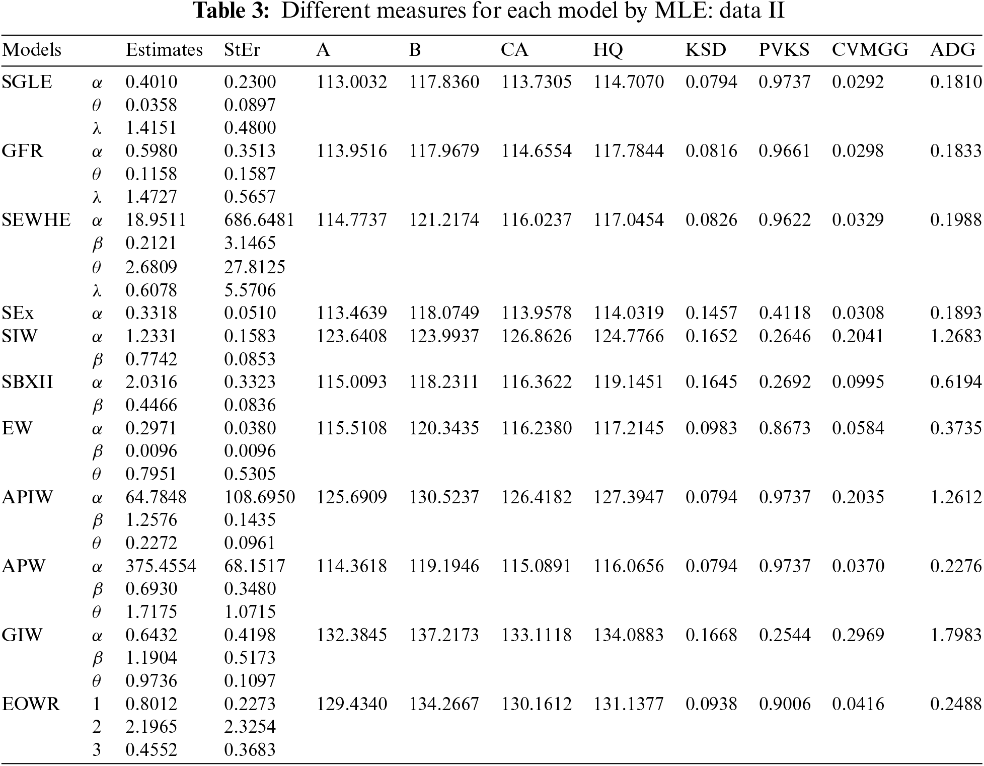
The SGLE model seeks to be employed in practical settings, such as the fit of real-world data, thanks to its desirable flexible qualities. We discuss this finding after taking into account the two well-cited real-world data sets below. Nine more effective models that have two or three tuning parameters and are expanded or modified versions of the exponential model are also taken into account for comparison. Namely, we consider generalized failure rate distribution (GFR), exponentiated Weibull-H exponential (SEWHE) [41], distribution, sine exponential (SEx) [42] distribution, alpha-sine Weibull (ASW) [43], sine-inverse Weibull (SIW) [44], sine-Burr XII (SBXII) [45], exponentiated Weibull (EW) [46], alpha power inverse Weibull (APIW) [47], alpha power Weibull (APW) [48], generalized inverse Weibull (GIW) [49], extended odd Weibull Rayleigh (EOWR) [50] distributions.

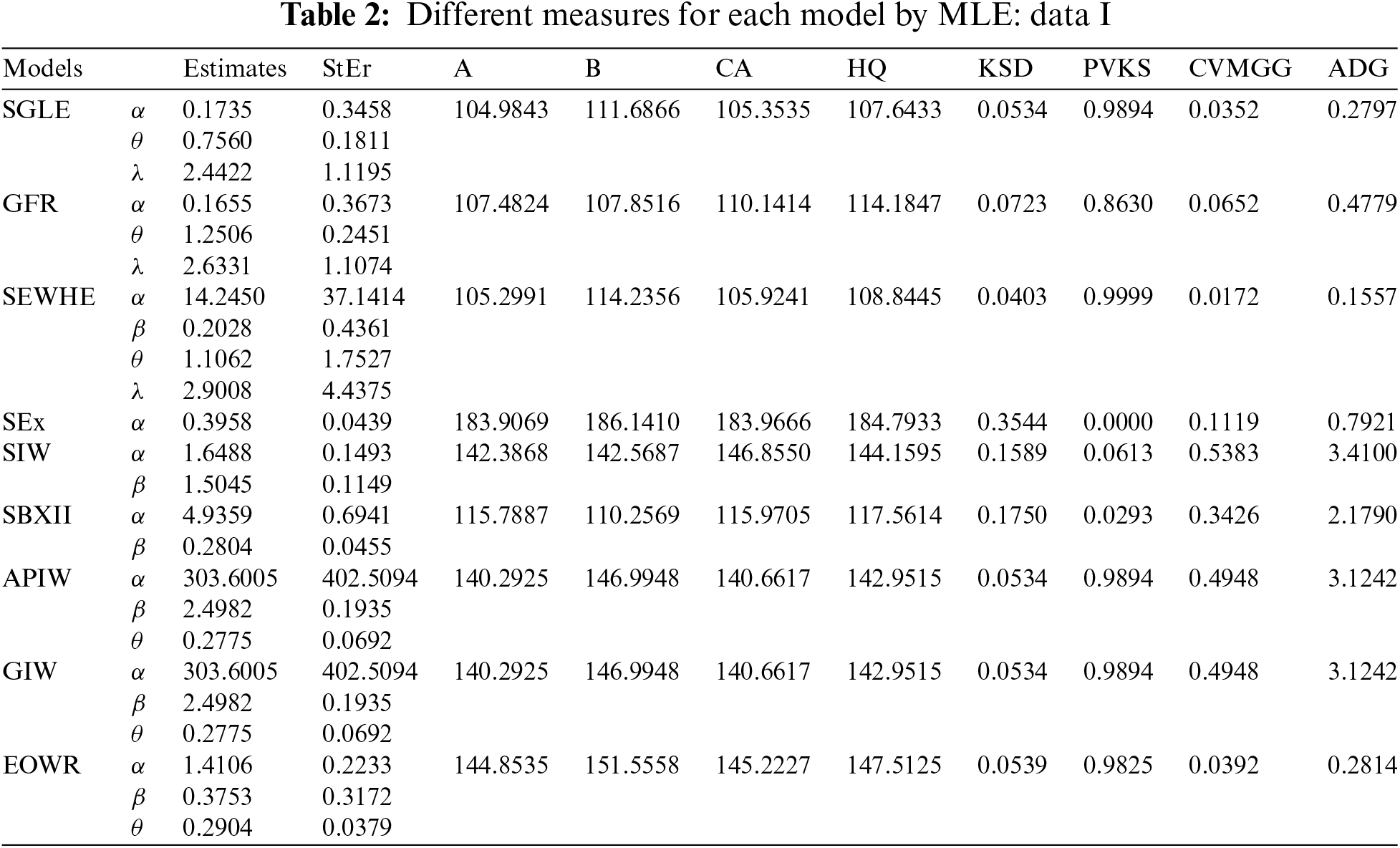
Akaike’s (A), Bayesian (B), Consistent Akaike’s (CA), and Hannan-Quinn (HQ) model selection information criteria are all used to demonstrate the utility of the SGLE distribution in contrast to competing models. To evaluate the validity of the SGRF model in contrast to other competing models, three additional goodness-of-fit statistics are also used: “Anderson-Darling (ADG), Cramer-von Mises (CVMG), and Kolmogorov-Smirnov (KSD) (with its p-value (PVKS))”. We used the R software along with the “AdequacyModel” package to estimate all unknown parameters through the maximum likelihood method. The standard errors (StEr) for these parameters were also computed and are reported in Tables 2 and 3. Based on these computations, the optimal distribution corresponds to the lowest values of A, B, CA, HQ, ADG, CVMG, and KSD statistics, along with the highest p-value. However, the estimated values of these goodness-of-fit measures for the various datasets are presented in Tables 2 and 3.

The first set of data: The first data set has been obtained by reference [51] as its source. It includes the single carbon fibre tensile strength (in GPa). Data I: “0.312, 0.314, 0.479, 0.552, 0.700, 0.803, 0.861, 0.865, 0.944, 0.958, 0.966, 0.997, 1.006, 1.021, 1.027, 1.055, 1.063, 1.098, 1.140, 1.179, 1.224, 1.240, 1.253, 1.270, 1.272, 1.274, 1.301, 1.301, 1.359, 1.382, 1.382, 1.426, 1.434, 1.435, 1.478, 1.490, 1.511, 1.514, 1.535, 1.554, 1.566, 1.570, 1.586, 1.629, 1.633, 1.642, 1.648, 1.684, 1.697, 1.726, 1.770, 1.773, 1.800, 1.809, 1.818, 1.821, 1.848, 1.880, 1.954, 2.012, 2.067, 2.084, 2.090, 2.096, 2.128, 2.233, 2.433, 2.585, 2.585”. The result of this application has baen presented by Table 2 and Figs. 4–8.

Figure 4: Fitted application for the SGLE distribution of data I with different graph

Figure 5: Profile MLE for for the SGLE parameters of data I

Figure 6: Uniqueness property MLE for the SGLE parameters of data I

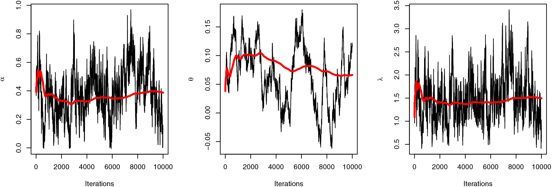
Figure 7: Trace plot of Bayesian estimators for the SGLE parameters: data I

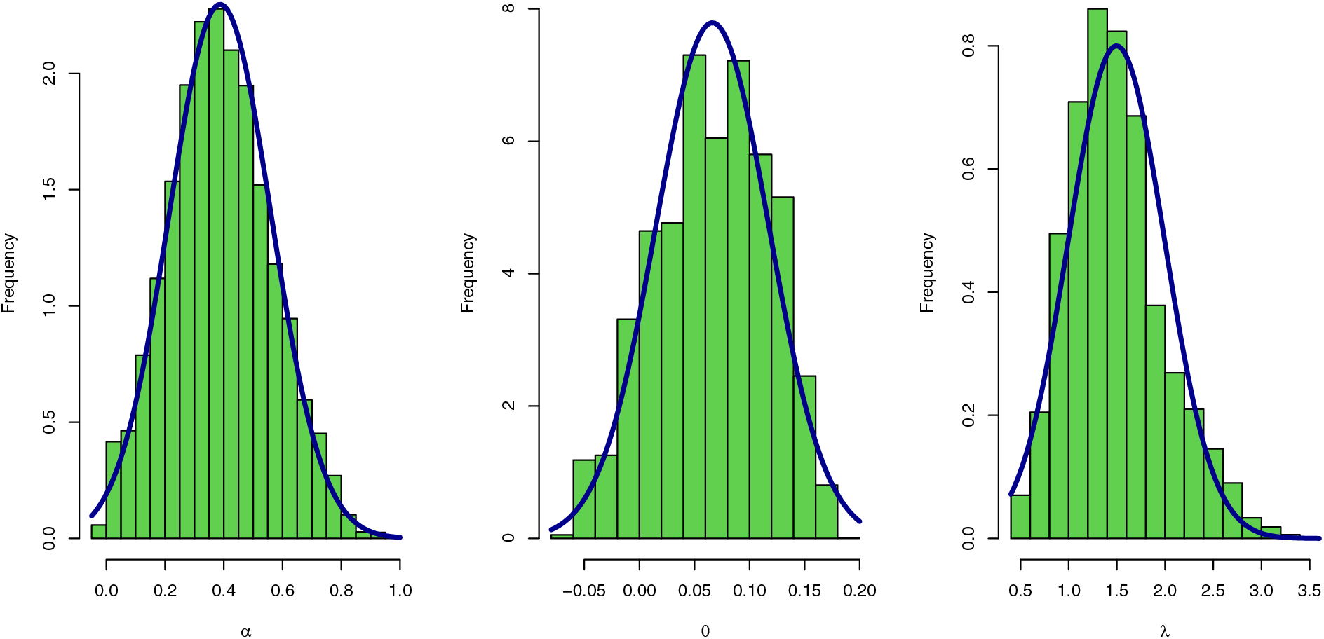
Figure 8: Histogram plot with normal curve of Bayesian estimators for the SGLE parameters: data I

To check the estimators by MLE for the SGLE parameters of data set I, Figs. 5, and 6 have been plotted to check these estimators have maximum and uniqueness values of MLE. Also, to check the estimators by Bayesian, Figs. 7, and 8 have been plotted to check these estimators have convergence and normality shapes of Bayesian estimates for the SGLE parameters.

The second data set, which can be accessible on June 30 2022, (see https://dataverse.harvard.edu/) shows the TFP growth in agricultural production for 37 African nations between 2001 and 2010. Data II: “4.6, 0.9, 1.8, 1.4, 0.2, 3.9, 1.8, 0.8, 2.0, 0.8, 1.6, 0.8, 2.0, 1.6, 0.5, 0.1, 2.5, 2.4, 0.6, 1.1, 0.7, 1.7, 1.0, 1.7, 2.5, 3.5, 0.3, 0.9, 2.3, 0.5, 1.5, 5.1, 0.2, 1.5, 3.3, 1.4, 3.3”. The result of this application has been presented by Table 3 and Figs. 9–13.

Figure 9: Fitted application for the SGLE distribution of data II with different graph

Figure 10: Profile MLE for the SGLE parameters of data II

Figure 11: Uniqueness property MLE for the SGLE parameters of data II

Figure 12: Trace plot of Bayesian estimators for the SGLE parameters: data II

Figure 13: Histogram plot with normal curve of Bayesian estimators for the SGLE parameters: data II

To check the estimators by MLE for the SGLE parameters of data set II, Figs. 10, and 11 have been plotted to check these estimators have maximum and uniqueness values of MLE. Also, to check the estimators by Bayesian for data set II, Figs. 12, and 13 have been plotted to check these estimators have convergence and normality shapes of Bayesian estimates for the SGLE parameters.

It is obvious that, when compared to the other distributions under the different data sets, the SGLE distribution is the best distribution. On the basis of the same data, we also create a fitted/empirical CDF, histogram, fitted density, PP plot, and quantile-quantile plots of the SGLE distribution (see Figs. 4 and 9). The results in Tables 2 and 3 show that the SGLE distribution is the most effective model to fit the various data when compared to all other given distributions indicated in Tables 2 and 3. Graphical representations in Figs. 4 and 9 support these findings.

8  Simulation

This section compares MLE and Bayesian estimates of the SGLE distribution parameter using Monte Carlo simulations using progressive Type-II censored samples. The simulation results are run in order to investigate and output in terms of mean square error (ω2), relative absolute bias (ω1), length confidence interval (ω3), and coverage probability of a confidence interval (ω4). We generate ten thousand random samples from the SGLE distribution for numerous individual parameters. For various sample sizes, n=40,70,100,150, and 200, failure censored sample m and different scheme, including:

Scheme (R) I: Rm=n−m, Ri=0;i=1,…,m−1.

Scheme (R) II: R1=n−m, Ri=0;i=2,…,m.

Complete: m=n, where Ri=0;i=1,…,m.

For the random variables generating, the values of the parameters α,θ, and λ are chosen as follows:

Case 1: α=0.5,θ=0.6,λ=0.5.

Case 2: α=0.5,θ=0.6,λ=2.2.

Case 3: α=0.5,θ=1.8,λ=0.5.

Case 4: α=1.1,θ=0.8,λ=0.9.

All necessary calculations were conducted utilizing R 4.3.0 software, employing three beneficial packages: the ‘coda’ package (MCMC by M-H algorithm) to make some Bayesian inference, the (maxLik) package (Newton-Raphson algorithm) to obtain likelihood inference, and the spread, skewness, and kurtosis of data sets encountercensored’ package to generate censored samples. Selecting initial parameter values involves options like leveraging domain knowledge, employing guess-and-check techniques, initiating random values within a defined range, executing grid searches in discrete parameter spaces, utilizing optimization algorithms for value generation, conducting sensitivity analyses for robustness, and referencing values from prior studies. The chosen method depends on the problem context, optimization algorithm, and parameter specifics, often prompting the exploration of multiple approaches. In our simulation study, we employed the guess-and-check method alongside optimization algorithms, specifically utilizing the “nlminb” function for generating initial values.

The following is a summary of Tables 4–7 included in the observations that follow:

•   As the sample size grows, the ω2, ω1, and LCI drop.

•   As the number of steps (m) rises, the ω1, ω2, and LCI drop.

•   For the majority of analysed cases of the SGLE distribution under progressively Type-II censored data, the Bayesian estimates are more effective than alternative approaches.

9  Conclusion

In this paper, we suggest a novel modification of the generalized linear exponential distribution termed the sine generalized linear exponential distribution, which makes use of the sine transformation’s features. The new distribution is extremely versatile and may be used to simulate survival data and reliability difficulties successfully. Depending on its settings, the new proposed model may have a rising, J-shaped HRF. As special sub-models, it incorporates various well-known lifespan distributions. The suggested model’s statistical features are described in detail. Under progressively censored data, the model parameters are addressed using maximum likelihood and Bayesian estimate approaches. We give simulated data to put these strategies to the test. Two real-world dataset applications highlight the importance of the newly presented model when compared to numerous regarded comparable models.

Acknowledgement: This work was supported and funded by the Deanship of Scientific Research at Imam Mohammad Ibn Saud Islamic University (IMSIU) (Grant Number IMSIU-RG23142).

Funding Statement: This work was supported and funded by the Deanship of Scientific Research at Imam Mohammad Ibn Saud Islamic University (IMSIU) (Grant Number IMSIU-RG23142).

Author Contributions: The authors confirm contribution to the paper as follows: study conception and design: N. A., A. S. A., I. E., M. E., E. M. A.; data collection: N. A., A. S. A., I. E., M. E., E. M. A.; analysis and interpretation of results: N. A., A. S. A., I. E., M. E., E. M. A.; draft manuscript preparation: N. A., A. S. A., I. E., M. E., E. M. A. All authors reviewed the results and approved the final version of the manuscript.

Availability of Data and Materials: The data mentioned in application section.

Conflicts of Interest: The authors declare that they have no conflicts of interest to report regarding the present study.

References

1. Sarhan, A. M., Kundu, D. (2009). Generalized linear failure rate distribution. Communications in Statistics-Theory and Methods, 38(5), 642–660. https://doi.org/10.1080/03610920802272414 [Google Scholar] [CrossRef]

2. Mahmoud, M., Alam, F. M. A. (2010). The generalized linear exponential distribution. Statistics & Probability Letters, 80(11), 1005–1014. [Google Scholar]

3. Jafari, A. A., Mahmoudi, E. (2022). Beta-linear failure rate distribution and its applications. Journal of the Iranian Statistical Society, 14(1), 89–105. [Google Scholar]

4. Sarhan, A. M., Ahmad, A. E. B. A., Alasbahi, I. A. (2013). Exponentiated generalized linear exponential distribution. Applied Mathematical Modelling, 37(5), 2838–2849. https://doi.org/10.1016/j.apm.2012.06.019 [Google Scholar] [CrossRef]

5. El-Damcese, M. A., Mustafa, A., El-Desouky, B. S., Mustafa, M. E. (2016). The odd generalized exponential linear failure rate distribution. Journal of Statistics Applications and Probability, 5, 299–309. [Google Scholar]

6. Luguterah, A., Nasiru, S. (2017). The odd generalized exponential generalized linear exponential distribution. Journal of Statistics Applications and Probability, 6, 139–148. https://doi.org/10.18576/jsap/060112 [Google Scholar] [CrossRef]

7. Mahmoud, M. A. W., Ghazal, M. G. M., Radwan, H. M. M. (2017). Inverted generalized linear exponential distribution as a lifetime model. Applied Mathematics & Information Sciences, 11, 1747–1765. [Google Scholar]

8. Okasha, H. M., Kayid, M. (2016). A new family of marshall-olkin extended generalized linear exponential distribution. Journal of Computational and Applied Mathematics, 296, 576–592. https://doi.org/10.1016/j.cam.2015.10.017 [Google Scholar] [CrossRef]

9. Alsadat, N., Elgarhy, M., Hassan, A. S., Ahmad, H., El-Hamid Eisa, A. (2023). A new extension of linear failure rate distribution with estimation, simulation, and applications. AIP Advances, 13(10), 105019. https://doi.org/10.1063/5.0170297 [Google Scholar] [CrossRef]

10. Jamal, F., Elbatal, I., Chesneau, C., Elgarhy, M., Hassan, A. (2019). Modified beta generalized linear failure rate distribution: Theory and applications. Journal of Prime Research in Mathematics, 15(1), 21–48. [Google Scholar]

11. Marshall, A. W., Olkin, I. (1997). A new method for adding a parameter to a family of distributions with application to the exponential and weibull families. Biometrika, 84(3), 641–652. https://doi.org/10.1093/biomet/84.3.641 [Google Scholar] [CrossRef]

12. Nicholas Eugene, C. L., Famoye, F. (2002). Beta-normal distribution and its applications. Communications in Statistics-Theory and Methods, 31(4), 497–512. https://doi.org/10.1081/STA-120003130 [Google Scholar] [CrossRef]

13. Cordeiro, G. M., de Castro, M., (2011). A new family of generalized distributions. Journal of Statistical Computation and Simulation, 81(7), 883–898. https://doi.org/10.1080/00949650903530745 [Google Scholar] [CrossRef]

14. Torabi, H., Montazeri, N. H. (2014). The logistic-uniform distribution and its applications. Communications in Statistics-Simulation and Computation, 43(10), 2551–2569. https://doi.org/10.1080/03610918.2012.737491 [Google Scholar] [CrossRef]

15. Cordeiro, G. M., Ortega, E. M. M., da Cunha, D. C. C. (2022). The exponentiated generalized class of distributions. Journal of Data Science, 11(1), 1–27. [Google Scholar]

16. Bourguignon, M., Silva, R. B., Cordeiro, G. M. (2022). The weibull-G family of probability distributions. Journal of Data Science, 12(1), 53–68. [Google Scholar]

17. Tahir, M. H., Cordeiro, G. M., Alzaatreh, A., Mansoor, M., Zubair, M. (2016). The logistic-X family of distributions and its applications. Communications in Statistics-Theory and Methods, 45(24), 7326–7349. https://doi.org/10.1080/03610926.2014.980516 [Google Scholar] [CrossRef]

18. Jamal, F., Nasir, M. A., Ozel, G., Elgarhy, M., Khan, N. M. (2019). Generalized inverted Kumaraswamy generated family of distributions: Theory and applications. Journal of Applied Statistics, 46(16), 2927–2944. https://doi.org/10.1080/02664763.2019.1623867 [Google Scholar] [CrossRef]

19. Afify, A. Z., Cordeiro, G. M., Ibrahim, N. A., Jamal, F., Elgarhy, M. et al. (2021). The Marshall-Olkin Odd Burr III-G family: Theory, estimation, and engineering applications. IEEE Access, 9, 4376–4387. https://doi.org/10.1109/ACCESS.2020.3044156 [Google Scholar] [CrossRef]

20. Al-Mofleh, H., Elgarhy, M., Afify, Z. A., Zannon, M. (2020). Type II exponentiated half logistic generated family of distributions with applications. Electronic Journal of Applied Statistical Analysis, 13(2), 536–561. [Google Scholar]

21. Ahmad, Z., Elgarhy, M., Hamedani, G., Butt, N. S. (2020). Odd generalized N-H generated family of distributions with application to exponential model. Pakistan Journal of Statistics and Operation Research, 16(1), 53–71. [Google Scholar]

22. Almarashi, A., Jamal, F., Chesneau, C., Elgarhy, M. (2021). A new truncated muth generated family of distributions with applications. Complexity, 2021, 1211526. https://doi.org/10.1155/2021/1211526 [Google Scholar] [CrossRef]

23. Abonongo, A. I. L., Abonongo, J. (2024). Exponentiated generalized weibull exponential distribution: Properties, estimation and applications. Computational Journal of Mathematical and Statistical Sciences, 3(1), 57–84. https://doi.org/10.21608/cjmss.2023.243845.1023 [Google Scholar] [CrossRef]

24. El-Sherpieny, E. S. A., Muhammed, H. Z., Almetwally, E. M. (2023). A new inverse rayleigh distribution with applications of COVID-19 data: Properties, estimation methods and censored sample. Electronic Journal of Applied Statistical Analysis, 16(2), 449–472. [Google Scholar]

25. Kumar, D., Singh, U., Singh, S. K. (2015). A new distribution using sine function its application to bladder cancer patients data. Journal of Statistics Applications & Probability, 4(3), 417–427. [Google Scholar]

26. Nadarajah, S., Kotz, S. (2006). Beta trigonometric distribution. Portuguese Economic Journal, 5(3), 207–224. https://doi.org/10.1007/s10258-006-0013-6 [Google Scholar] [CrossRef]

27. Kharazmi, O., Saadatinik, A. (2016). Hyperbolic cosine-F family of distributions with an application to exponential distribution. Gazi University Journal of Science, 29(4), 811–829. [Google Scholar]

28. Kharazmi, O., Saadatinik, A., Alizadeh, M., Hamedani, G. G. (2019). Odd hyperbolic cosine-FG family of lifetime distributions. Journal of Statistical Theory and Applications, 18, 387–401. https://doi.org/10.2991/jsta.d.191112.003 [Google Scholar] [CrossRef]

29. Kharazmi, O., Saadatinik, A., Jahangard, S. (2019). Odd hyperbolic cosine exponential-exponential (OHC-EE) distribution. Annals of Data Science, 6, 765–785. https://doi.org/10.1007/s40745-019-00200-z [Google Scholar] [CrossRef]

30. He, W., Ahmad, Z., Afify, A. Z., Goual, H. (2020). The arcsine exponentiated-X family: Validation and insurance application. Complexity, 2020, 8394815. https://doi.org/10.1155/2020/8394815 [Google Scholar] [CrossRef]

31. Balakrishnan, N., Aggarwala, R. (2000). Progressive censoring: theory, methods, and applications, pp. 11–29. Boston: Birkhauser. [Google Scholar]

32. Balakrishnan, N., Sandhu, R. A. (1995). A simple simulational algorithm for generating progressive Type-II censored samples. The American Statistician, 49(2), 229–230. https://doi.org/10.1080/00031305.1995.10476150 [Google Scholar] [CrossRef]

33. Aggarwala, R., Balakrishnan, N. (1996). Recurrence relations for single and product moments of progressive type-II right censored order statistics from exponential and truncated exponential distributions. Annals of the Institute of Statistical Mathematics, 48(4), 757–771. https://doi.org/10.1007/BF00052331 [Google Scholar] [CrossRef]

34. Aggarwala, R., Balakrishnan, N. (1998). Some properties of progressive censored order statistics from arbitrary and uniform distributions with applications to inference and simulation. Journal of Statistical Planning and Inference, 70(1), 35–49. https://doi.org/10.1016/S0378-3758(97)00173-0 [Google Scholar] [CrossRef]

35. Balakrishnan, N., Kannan, N., Lin, C., Ng, H. (2003). Point and interval estimation for gaussian distribution, based on progressively Type-II censored samples. IEEE Transactions on Reliability, 52(1), 90–95. https://doi.org/10.1109/TR.2002.805786 [Google Scholar] [CrossRef]

36. Maiti, K., Kayal, S. (2021). Estimation of parameters and reliability characteristics for a generalized rayleigh distribution under progressive Type-II censored sample. Communications in Statistics-Simulation and Computation, 50(11), 3669–3698. https://doi.org/10.1080/03610918.2019.1630431 [Google Scholar] [CrossRef]

37. Muhammed, H. Z., Almetwally, E. M. (2024). Bayesian and non-bayesian estimation for the shape parameters of new versions of bivariate inverse weibull distribution based on progressive Type II censoring. Computational Journal of Mathematical and Statistical Sciences, 3(1), 85–111. https://doi.org/10.21608/cjmss.2023.250678.1028 [Google Scholar] [CrossRef]

38. Okasha, H., Nassar, M. (2023). On a new version of weibull model: Statistical properties, parameter estimation and applications. Computer Modeling in Engineering & Sciences, 137(3), 2219–2241. https://doi.org/10.32604/cmes.2023.028783 [Google Scholar] [CrossRef]

39. Algarni, A., Almarashi, A. M. (2022). A new rayleigh distribution: Properties and estimation based on progressive Type-II censored data with an application. Computer Modeling in Engineering & Sciences, 130(1), 379–396. https://doi.org/10.32604/cmes.2022.017714 [Google Scholar] [CrossRef]

40. Henningsen, A., Toomet, O. (2011). maxLik: A package for maximum likelihood estimation in R. Computational Statistics, 26, 443–458. https://doi.org/10.1007/s00180-010-0217-1 [Google Scholar] [CrossRef]

41. Alyami, S. A., Elbatal, I., Alotaibi, N., Almetwally, E. M., Elgarhy, M. (2022). Modeling to factor productivity of the United Kingdom food chain: Using a new lifetime-generated family of distributions. Sustainability, 14(14), 8942. https://doi.org/10.3390/su14148942 [Google Scholar] [CrossRef]

42. Park, J. C., Lim, H. Y., Kang, D. S. (2021). Predicting rebar endpoints using sin exponential regression model. http://arxiv.org/abs/2110.08955 [Google Scholar]

43. Benchiha, S., Sapkota, L. P., Al Mutairi, A., Kumar, V., Khashab, R. H. et al. (2023). A new sine family of generalized distributions: Statistical inference with applications. Mathematical and Computational Applications, 28(4), 83. https://doi.org/10.3390/mca28040083 [Google Scholar] [CrossRef]

44. Souza, L., Junior, W., de Brito, C., Chesneau, C., Ferreira, T. et al. (2019). On the Sin-G class of distributions: Theory, model and application. Journal of Mathematical Modeling, 7(3), 357–379 [Google Scholar]

45. Isa, A. M., Ali, B. A., Zannah, U. (2022). Sine burr xii distribution: Properties and application to real data sets. Arid-Zone Journal of Basic & Applied Research, 1, 48–58. [Google Scholar]

46. Pal, M., Ali, M. M., Woo, J. (2006). Exponentiated weibull distribution. Statistica, 66(2), 139–147. [Google Scholar]

47. Basheer, A. M. (2019). Alpha power inverse weibull distribution with reliability application. Journal of Taibah University for Science, 13(1), 423–432. https://doi.org/10.1080/16583655.2019.1588488 [Google Scholar] [CrossRef]

48. Nassar, M., Alzaatreh, A., Mead, M., Abo-Kasem, O. (2017). Alpha power weibull distribution: Properties and applications. Communications in Statistics-Theory and Methods, 46(20), 10236–10252. https://doi.org/10.1080/03610926.2016.1231816 [Google Scholar] [CrossRef]

49. de Gusmão, F., Ortega, E., Cordeiro, G. (2011). The generalized inverse weibull distribution. Statistical Papers, 52, 591–619. https://doi.org/10.1007/s00362-009-0271-3 [Google Scholar] [CrossRef]

50. Almetwally, E. M. (2021). Extended odd weibull inverse rayleigh distribution with application on carbon fibres. Mathematical Sciences Letters, 10(1), 5–14. https://doi.org/10.18576/msl [Google Scholar] [CrossRef]

51. Mohammad, Z., Raqab, M. T. M., Kundu, D. (2008). Estimation of P(Y < X) for the three-parameter generalized exponential distribution. Communications in Statistics-Theory and Methods, 37(18), 2854–2864. [Google Scholar]