
 Submit a Paper
 Propose a Special lssue
 Open Access
ARTICLE

A Hybrid Approach for Predicting the Remaining Useful Life of Bearings Based on the RReliefF Algorithm and Extreme Learning Machine
1 School of Mechatronics Engineering, Anhui University of Science and Technology, Huainan, 232001, China
2 Institute of Energy, Hefei Comprehensive National Science Center, Hefei, 230031, China
* Corresponding Authors: Sen-Hui Wang. Email: ; Ke Yang. Email:
Computer Modeling in Engineering & Sciences 2024, 140(2), 1405-1427. https://doi.org/10.32604/cmes.2024.049281
Received 02 January 2024; Accepted 25 March 2024; Issue published 20 May 2024
 View Full Text
 Download PDF
Abstract
Accurately predicting the remaining useful life (RUL) of bearings in mining rotating equipment is vital for mining enterprises. This research aims to distinguish the features associated with the RUL of bearings and propose a prediction model based on these selected features. This study proposes a hybrid predictive model to assess the RUL of rolling element bearings. The proposed model begins with the pre-processing of bearing vibration signals to reconstruct sixty time-domain features. The hybrid model selects relevant features from the sixty time-domain features of the vibration signal by adopting the RReliefF feature selection algorithm. Subsequently, the extreme learning machine (ELM) approach is applied to develop a predictive model of RUL based on the optimal features. The model is trained by optimizing its parameters via the grid search approach. The training datasets are adjusted to make them most suitable for the regression model using the cross-validation method. The proposed hybrid model is analyzed and validated using the vibration data taken from the public XJTU-SY rolling element-bearing database. The comparison is constructed with other traditional models. The experimental test results demonstrated that the proposed approach can predict the RUL of bearings with a reliable degree of accuracy.Keywords
Supplementary Material
Supplementary Material FileNomenclature
| Acronyms | |
| RUL | Remaining useful life |
| ELM | Extreme learning machine |
| ANN | Artificial neural network |
| SVR | Support vector regression |
| SLFN | Single-hidden-layer feedforward neural network |
| MAE | Mean absolute error |
| RMSE | Root mean square error |
| R2 | Coefficient of determination |
| Notation | |
| Di | The ith sample |
| t | The number of total samples |
| k | The number of samples nearest to the ith sample |
| P | The output indicator of the sample |
| P0 | The value of the output indicator P of sample Di |
| A | The input feature of the sample |
| ndC | The weight for different prediction values |
| ndA[A] | The weight for different features |
| ndC&dA[A] | The weight for different predictions and different features |
| W[A] | The weight value of input feature A |
| (xi, yi) | The sample of the dataset |
| m | The number of output nodes |
| n | The number of input nodes |
| L | The number of hidden nodes |
| g(., ., .) | The nonlinear activation function |
| wi | The weight vector that connects the input layer and hidden layer |
| b | The bias of the hidden nodes |
| β | The weight vector that connects the hidden layer and output layer |
| h(x) | The output of the hidden layer |
| H | The output matrix of the hidden layer |
| H† | The Moore-Penrose generalized inverse of matrix H |
| HT | The transpose of matrix H |
| C | The regularization coefficient |
| I | The identity matrix |
| γ | The kernel parameter for the SVR algorithm |
Bearings are common essential components in mining rotating equipment subjected to continuous high-load working conditions over a long time. Based on statistics, bearing faults can account for over 40% of all machine faults [1], almost 40%–50% of all motor failures [2], and over 70% of wind turbine gearbox failures [3]. Accordingly, the phase of the bearings significantly affects the regular operation of the entire mechanical system. Therefore, the study of the condition monitoring and fault diagnosis technology of mechanical equipment has attracted increasing attention in bearing maintenance.
A prognosis maintenance policy characterizes the deterioration process of rotating equipment and computes the predicted time for the indicator to arrive at the failure threshold. It determines the current status of a device and estimates its lifespan before a fault occurs. This study estimates the RUL of roll element bearings by feature selection based on time domain signals. The proposed RUL prediction model improves the reliability of mechanical systems.
The methods employed to estimate the RUL of bearings can be classified into three categories: model-based, data-driven, and a combination of the above approaches [4,5].
The model-based method is applied to construct a failure model based on physical principles with some mathematical formulas. Liao et al. [6] introduced the proportional hazards and logistic regression models for RUL prediction. Liao [7] proposed a genetic programming method to discover the advanced features in RUL prediction. Li et al. [8] improved the exponential model and utilized it to predict the RUL of rolling element bearings. Jantunen et al. [9] presented an approach to understanding the wear of bearings and applied it to predict the RUL of rolling element bearings. Lei et al. [10] proposed a nonlinear degradation model for RUL prediction of bearings. Kumar et al. [11] established a novel health degradation indicator to estimate the RUL of bearings. Teng et al. [12] developed a robust model-based approach for bearing life prognosis in wind turbines. Lei et al. [13] introduced the weighted minimum quantization error as a health indicator to construct a model-based model for estimating the RUL of machinery. Pan et al. [14] constructed an inverse Gaussian degradation model to predict the RUL of a deteriorating system. Wang et al. [15] employed an exponential model combined with a gradient approach to determine the preliminary prediction time and further estimate the RUL of rolling bearings. However, it is difficult to establish a mathematical model that includes all the physical laws and failure mechanisms. This is because the system structure is highly complex with variable operating conditions; thus, the specific models are different for each system. In addition, it is costly to develop such physical failure models.
Data-driven methods are more appropriate for fault diagnosis based on historical data in complex systems. Meng et al. [16] proposed a novel convolution network based on a temporal attention fusion mechanism to predict the RUL of bearings. Zhu et al. [17] proposed a dynamically activated convolutional network for the RUL prediction of rolling bearing. Yang et al. [18] improved the long short-term memory with uncertain quantification and applied it to predict the RUL of bearings. Wang et al. [19] proposed a model that combined multiscale fusion permutation entropy with multiscale convolutional attention neural networks for predicting RUL of bearings. Jiang et al. [20] provided the remaining life prediction method with the assistance of Bayesian short-term and long-term memory neural networks. Li et al. [21] established a gated recurrent unit-deep autoregressive model with an adaptive failure threshold to predict the RUL of rolling bearings. A model of the system behavior can be established based on the measurement data using data-driven approaches. Guo et al. [22] built a long short-term memory model based on an attention mechanism combined with empirical wavelet transform to predict the RUL of bearings. Zhang et al. [23] utilized the digital twin method to build the RUL prediction model. Wang et al. [24] constructed a bearing life prediction model based on an improved temporal convolutional network and transfer learning. Du et al. [25] established a convolutional neural network model based on a global attention mechanism for RUL prediction of bearings. Zou et al. [26] proposed a transfer prediction model based on the dynamic benchmark to predict the RUL of bearings. Du et al. [27] developed an angular domain unscented particle filter model with time-varying degradation parameters for RUL prediction of rolling bearings. Jin et al. [28] applied the Kolmogorov-Smirnov test to distinguish between different health statuses of bearings. They employed the unscented Kalman filter approach to select the appropriate parameters for the nonlinear degradation model, which can effectively predict the RUL of a bearing undergoing degradation. Pan et al. [29] divided the running process of a bearing into normal and degraded stages and constructed a two-stage predictive model using the relative root mean square value to estimate the RUL of rolling-element bearings. Kuo et al. [30] employed a dense-structured network method to predict the RUL of a bearing with a minimal amount of measurement data. Therefore, choosing the best features that can depict the bearing degradation process is essential to accurately capture bearing degradation information.
Accordingly, a data-driven model is constructed using the RReliefF method for feature dimension reduction combined with the ELM algorithm for estimating the RUL of bearings. In the proposed prediction model, the optimal feature set was selected from sixty-time domain features using the RRelifF feature selection algorithm. Subsequently, an ELM model was developed to estimate the RUL of rolling element bearings. To evaluate the predictive performance of the hybrid predictive model, ANN and SVR methods were constructed to perform a comprehensive comparison. A data set of rolling element bearings taken from the XJTU-SY database [31] was utilized to conduct the comparative experiments.
This study makes three primary contributions to the literature. (1) To address the difficulty in extracting features of vibration signals from the available degradation data of bearings, the RReliefF algorithm can be used for feature selection and search for the optimal feature subset. Accordingly, the RReliefF algorithm is adopted in this study to estimate the weight of time domain features. This can directly demonstrate the relevancy between time domain features and the RUL of bearings, presenting the optimal input feature set for the predictive model. (2) When training the predictive model, the training data set is not selected empirically but using the cross-validation method to establish a predictive model with the ability to make exact predictions using limited training samples. (3) The proposed hybrid method is thoroughly compared against the existing approaches to assess its effectiveness and robustness. Compared to traditional algorithms, the proposed hybrid predictive model achieves superior performance.
The remainder of this paper is organized as follows. Section 2 briefly introduces the basic theory of the RReliefF feature selection algorithm and ELM method. Section 3 presents the vibration data from the public XJTU-SY bearing database and sixty-feature reconstruction based on the time domain signals. Section 4 describes the implementation process of selecting the optimal feature subset and optimizing the parameters of the ELM, ANN, and SVR models. Section 5 provides a detailed explanation of the analysis and a discussion of the predictive model results. Eventually, conclusions are drawn in Section 6.
2 Theory of Feature Selection and Regression
2.1 RReliefF Feature Selection Algorithm
The RReliefF algorithm [32–34] selects the relevance of the features to solving a regression issue. The implementation steps of the RReliefF algorithm for regression tasks are stated as follows:
Step 1: Randomly select a sample Di (i = 1, 2,..., t) and select the k samples closest to Di from the remaining t-1 samples.
Step 2: Calculate the weight set ndC under the condition of P0 output index value of sample Di.
where P0 is the value of the output indicator P for sample Di; Pi is the indicator value for the ith sample in k samples; Pmin and Pmax are the minimum and maximum values for the output indicators in t samples, respectively.
Step 3: Calculate the weight set ndA[A] of input feature A for sample Di.
where A0 is the value of feature A for sample Di; Ai is the value of feature A for the ith sample in k samples; Amin and Amax are the minimum and maximum values of feature A in t samples, respectively.
Step 4: Calculate the weight set ndC&dA[A] of sample Di with respect to the output indicator P0 and input feature A.
Step 5: Repeat the previous four steps for a total of m times to obtain t ndC, t ndA[A], and t ndC&dA[A]. Then, calculate these t weight sets in sum to obtain NdC, NdA[A], and NdC&dA[A], respectively.
Step 6: Calculate the weight value W[A] of the input feature A.
The feature weights are calculated by the RReliefF algorithm within the range of [−1, 1] [35]. A weight of +1 indicates that different values of a feature correspond to various values of the target index for near-neighbor samples, while a weight of −1 represents that various values of a feature result in the same values of the target index for near-neighbor samples. Hence, the higher the score of the feature weight, the greater its impact on the regression issue. The weights of all the features were obtained using the RReliefF algorithm and can be sorted in descending order. The larger the weight, the greater the correlation with the corresponding feature.
The RReliefF algorithm is an alternative ReliefF algorithm introduced to solve regression problems and named the Regressional ReliefF algorithm. The primary purpose of the RReliefF algorithm is to identify the feasible features sensitive to RUL based on the reconstructed features of the vibration signal. In other words, the RReliefF is a feature selection algorithm utilized to distinguish the quality of features in problems with a strong correlation between the features. The operation process of the feature selection using RReliefF is stated as follows. Firstly, the weight scores of all the candidate features are calculated using the RReliefF algorithm. Secondly, all the candidate features are ranked by level of importance according to the value of the weight score. Thirdly, the most relevant features from the candidate are selected based on the rank sequence. Finally, the prediction model is constructed by training the ELM algorithm with the selected features.
The ELM established by Huang et al. [36] is an SLFN with fast learning speed and good generalization ability, providing a unified learning paradigm for regression or classification tasks. The implementation process of ELM [37–39] is stated as follows.
Given a regression task with N different data points (xi, yi), where xi = [xi1, xi2,..., xin]T ∈ Rn indicates n input nodes and yi = [yi1, yi2, ..., yim]T ∈ Rm indicates m output nodes, such that (xi, yi) ∈ Rn × Rm, i = 1, 2, ..., N. Let L be the number of hidden neurons and g(., ., .) be a nonlinear transfer function, then the output function of ELM is stated as follows:
where wi = [wi1, wi2, ..., win]T is the weight vector that connects the n input neurons into the ith hidden neuron; bi is the bias of the ith hidden neuron, both wi and bi are generated randomly, and i varies from 1 to L; β = [β1, β2, ..., βL]T is the weight vector that joins the hidden and output nodes.
The output function of the hidden layer in terms of the input vector x is defined as follows:
where the output function g(x) maps the n-dimensional input feature space to an L-dimensional feature space. The output matrix H of the hidden layer for the N input training samples is described as follows:
The ELM training task aims to ensure that the output of SLFN matches the target vector of the regression. Thus, the compact form of Eq. (5) can be rewritten as follows:
ELM aims to minimize the training error and norm of output weights as follows:
The output weight vector β can be solved by introducing the Moore-Penrose generalized inverse [40] as follows:
where H† is the Moore-Penrose generalized inverse of matrix H. The orthogonal projection approach can be employed to determine the Moore-Penrose generalized inverse of matrix H in two cases: when HTH is nonsingular and H† = (HT H)−1 HT, or when HHT is nonsingular and H† = HT(HHT)−1. To avoid overfitting of these implementations and improve the stability of the ELM, a positive parameter 1/C is introduced to calculate the output weight vector as follows:
or
where I is the identity matrix; C is the regularization coefficient that coordinates structural and experiential risk.
In these implementations, the input weight vector and hidden layer biases are randomly generated and do not consume more time than that required by back-propagation. The only two model parameters are the number of hidden neurons (L) and regularization coefficient (C); thus, the ELM is easy to implement without tuning the hidden layer. The critical step of ELM is to solve the Moore-Penrose generalized inverse of the output matrix H, which can avoid local minimization and achieve good performance under less human intervention. The two calculation approaches for the output weight vector can yield a high learning speed when dealing with a large volume of data. Using the L2-norm regularization in ELM enhances the sparsity of the output layer and produces an optimal solution with negligible errors.
The ELM algorithm is a network with one hidden layer comprising two parts of the work. Firstly, the network non-linearly maps the input vector into a high-dimensional feature space randomly through the hidden layer. Secondly, the regression task is accomplished by a supervised linear learner with the output layer. The sigmoid function is a typical nonlinear activation function used in the ELM algorithm. Based on the theory, the ELM works with high scalability and low computational complexity. In addition, the ELM provides a unified solution to different applications, such as regression, binary, and multiclass classifications. Compared to traditional machine learning algorithms, ELM tends to reach both the smallest training error and the norm of output weights. Thus, the ELM tends to have better generalization performance than the traditional learning algorithms.
All illustrations of ELM are shown in Fig. 1.
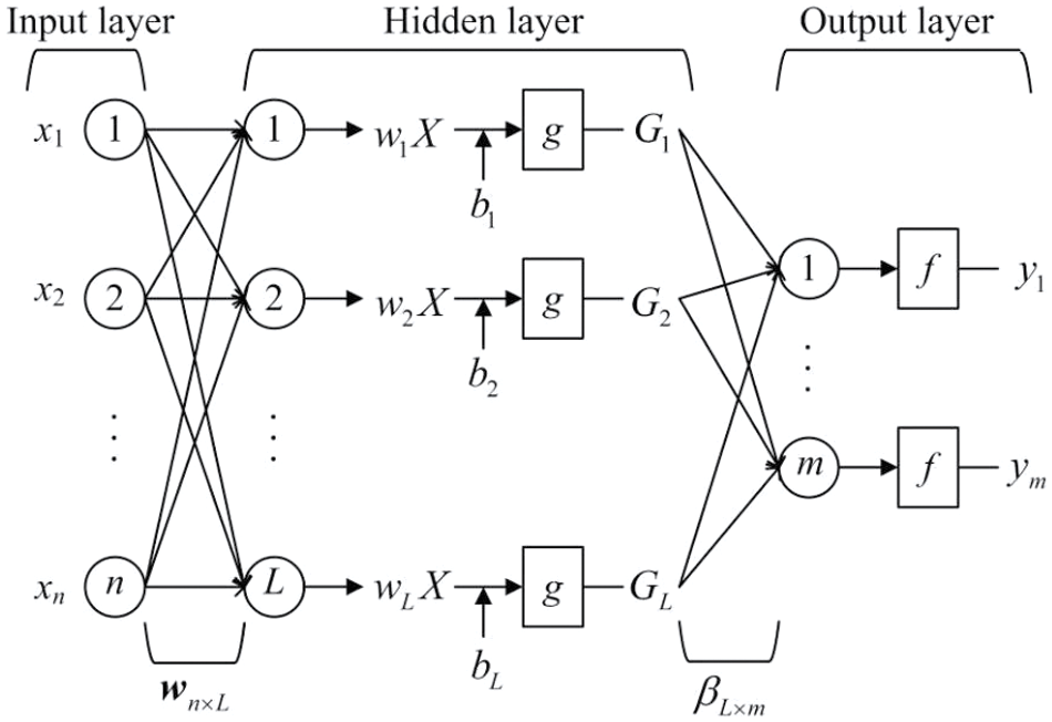
Figure 1: The illustration of ELM
The ELM algorithm initially evolved from the neural networks with a single hidden layer. The primary purpose of the ELM is to realize both the minimal training error and the minimal norm of output weights. The ELM algorithm is an effective solution for regression applications. Compared to conventional neural networks, ELM has milder optimization constraints, making ELM learning extremely fast and producing better generalization performance. The process of ELM can be briefly stated as follows. First, the input weights and the hidden biases are chosen randomly. The kernel parameters are tuned and can be fixed using the grid-search method. Second, the model is trained to find a least-squares solution of the linear output layer matrices. The output weights are analytically determined by the Moore-Penrose generalized inverse operation. Finally, the trained machine learning algorithm provides a unified platform for applying the RUL prediction issue practically.
This study used the bearing database established by Xi’an Jiao Tong University and Sum Yong Technology Co., Ltd. (China), defined as XJTU-SY [31]. The conceptual representation of the experimental platform is shown in Fig. 2. During the experiment, the bearing degradation process was monitored by an accelerometer sensor under different operating conditions (i.e., different radial force and rotational speed). The tested bearing type was LDK UER204; the comprehensive operating conditions are reported in Table 1. The database contains complete life cycle data for 15 rolling element bearings. The sample rate for the vibration signal is 25.6 kHz, and 32,768 data points (i.e., 1.28 s) are recorded every minute. As mentioned in the previous sections, the vibration signal is more helpful in monitoring bearing degradation when the load is exerted in the horizontal direction. Therefore, this study analyzed the horizontal vibration signals to create a predictive model regarding the RUL of bearings. Basedon the failure criterion, the moment when the value of the vibration signal exceeds 20 g is defined as the failure time of the experimental bearing. Fig. 3 displays typical horizontal and vertical vibration signals throughout the entire service life period monitored by the accelerometer. The amplitude of the vibration signals exhibits an increasing trend at the end of the experiment, indicating a quick degradation.
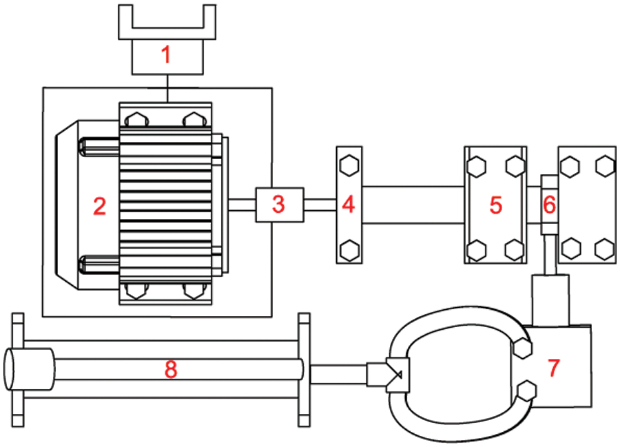
Figure 2: Conceptual representation of the experimental platform. (1: motor speed controller, 2: electric motor, 3: flexible coupling, 4, 5: support bearings, 6: test bearing, 7: hydraulic loading, 8: hydraulic manual pump)
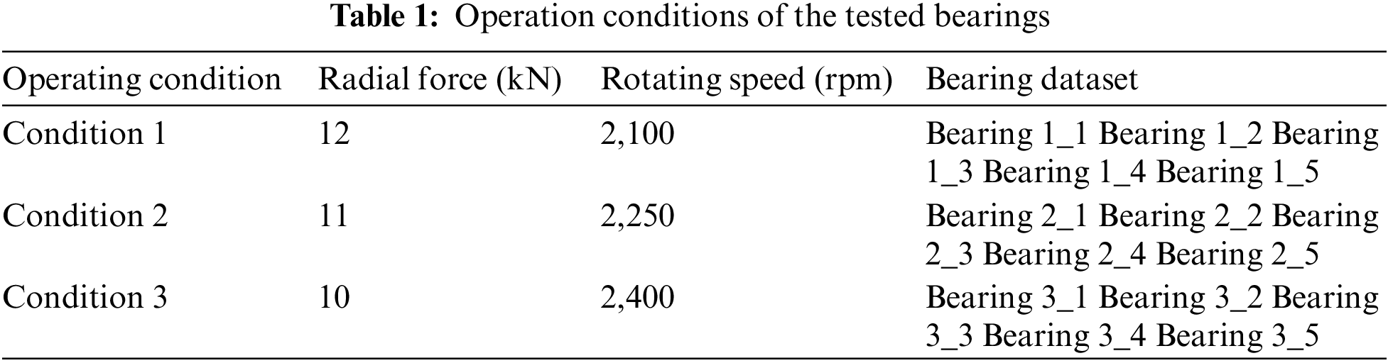
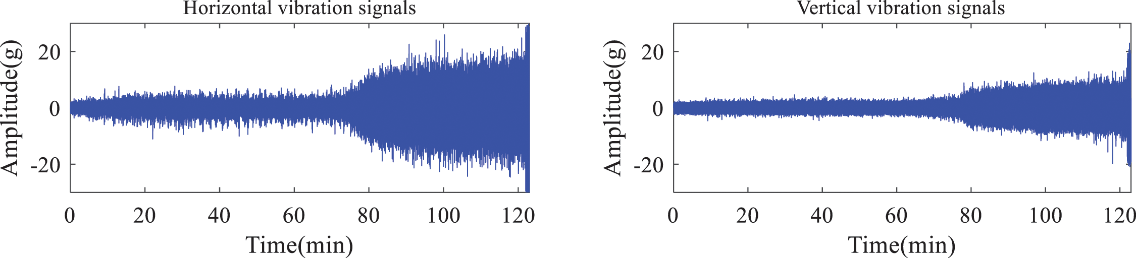
Figure 3: Typical horizontal and vertical vibration signals
In the XJTU-SY database, the sample rate for the vibration signal is 25.6 kHz, and a total of 32,768 data points (i.e., 1.28 s) are recorded every minute. Thus, the total data points in one minute are utilized to calculate the candidate input features. In other words, the data collected in one minute represents a sample. According to the failure criterion, the moment when the value of the vibration signal exceeds 20 g is defined as the failure time of the experimental bearing. Therefore, data with an amplitude not exceeding 20 g is selected as the full-life data of the bearing. The values of the RUL are calculated by y = i/N, where i is the ith sample, and N is the total of samples of the full-life data. This means that the initial value of RUL is close to 0, and the final value is 1. Hence, the output target index of the model is in the interval of [0,1].
The candidate input features used in the bearing degradation analysis are listed in Table 1 in the Appendix. Data normalization is crucial when the features of a data set have different numeric ranges. The primary purpose of normalization is to eliminate the dimensional and numerical differences between features. Another advantage is that the features have the same measurement scale and enable comparability between features with different dimensions. Therefore, all input features are normalized into the interval of [0,1].
The data normalization equation is performed as follows:
where xnormalize is the target value; x is the original data; xmin and xmax are the minimum and maximum values of the original data set, respectively. This equation normalized all input features into the interval of [0,1]. In contrast, this normalization method can highly match the value of the RUL used in this study. This normalization method can make calculating the errors easier.
4.1 Feature Selection Using the RReliefF Algorithm
The RReliefF algorithm is an effective solution for feature selection in regression problems. RReliefF estimates the quality of features and is applied to extract features with strong dependencies in a prepossessing step before the model is learned. The distance between the instances is considered in the RReliefF algorithm to evaluate the significance of features between the instances. To calculate the W[A] of the quality of feature A in regression applications, the probability of the predicted values of different samples is applied to model the relative distance between the predicted values of the different samples. This study applied RReliefF to rank the features of the time-domain vibration signals from the candidate sixty features set. The RReliefF algorithm assigns a weighted score W[A] to each feature based on how well it distinguishes between samples that are near to each other. Hence, the significant features can be extracted, and the model’s predictive performance can be improved further.
The primary purpose of feature selection is to select the most relevant features from many available features using the RReliefF algorithm. The procedure started with extracting the most relevant features from the candidate set, where the RReliefF feature selection algorithm was employed to rank features based on their weight scores. Second, an RUL prediction model was established by training the ELM algorithm using the candidate input features extracted in the first step. Within the training phase, the bearing data were split into three categories: training, validation, and testing datasets. The training and validation datasets were used in the feature selection process. If the regression error for validation data is lower than the predefined error, the regression predictor can be used for RUL prediction in rolling element bearings. Otherwise, a new feature should be reconstructed based on the calculated weights such that the regression predictor is retrained with the new feature set. At the RUL prediction stage, the test dataset of bearings can be input to the trained ELM regression predictor. For comparison, the ANN and SVR algorithms were fed with the same input features; thus, the results of these different models can be comparable with those of the ELM model.
The procedure of the proposed hybrid RUL prediction model is shown in Fig. 4. The RUL prediction procedure includes four phases: data collecting, data preprocessing, training, and RUL predicting phase. First, the experimental platform can obtain the sample data for the bearings under different operating conditions. The profiles involving horizontal and vertical vibration signals are edited to get the sample data within minutes. Second, the time-domain horizontal vibration signals are chosen as the analysis data for the RUL prediction model. Based on the sample data, the sixty time-domain features are calculated to form the candidate feature set. Third, in the training phase, the weight scores of the sixty features are calculated using the RReliefF algorithm, and the features that indicate the degradation states of bearings are extracted accordingly. The two user-defined parameters (regularization coefficient and hidden nodes) and the training set are optimally selected using the grid search method and cross-validation approach. Last, new test data collected from the experimental platform can be inputted to the trained ELM model for the RUL prediction in the RUL predicting phase.
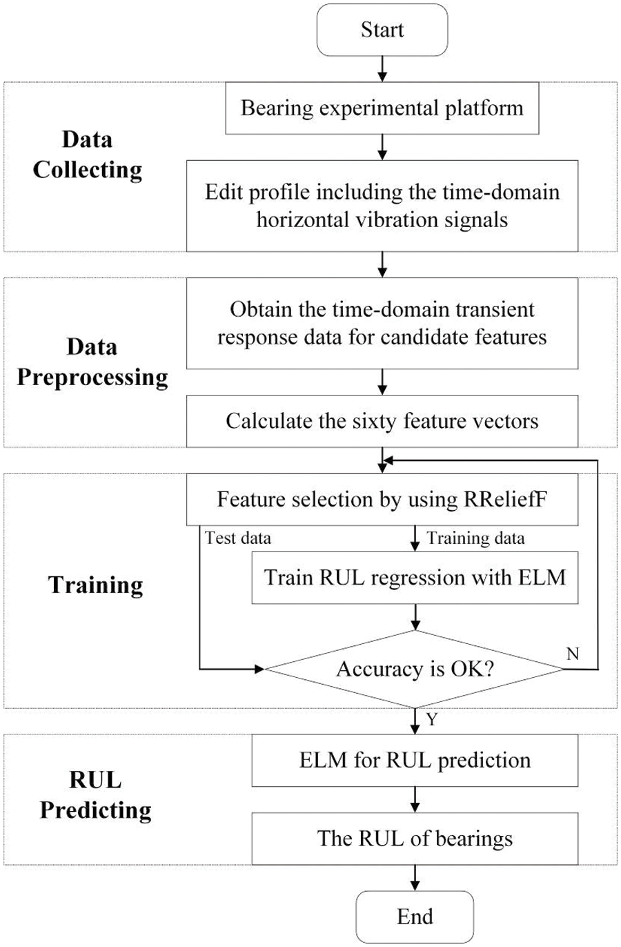
Figure 4: Flowchart of the proposed hybrid RUL prediction model
The RReliefF algorithm is one of the most successful feature selection algorithms. It works as a filter to estimate the importance of features to discard noisy features and improve the regression task to reduce the combinatorial explosion during the searching strategy. The RReliefF algorithm evaluates a feature’s importance by considering its dependence on other features. Therefore, the synergistic effect between features can be recognized. RReliefF algorithm aims to scale down the number of features, reducing thus the size of the multidimensional searching space. The ability of the RReliefF algorithm to discriminate the true feature from the basic candidate feature set is evaluated in bearing datasets. This study utilized the RReliefF algorithm to choose a small feature subset from the sixty candidate feature sets. This feature selection is necessary and sufficient to describe the RUL prediction of bearings using the vibration signal.
In the experiments, the performances of the three different methods were evaluated in terms of three measurements: the MAE, RMSE, and R2:
where yi is the actual value of the target index variable; f(xi) is the predicted value; r is the size of the data set.
In this study, the ELM algorithm is implemented because it can meet the requirements of the RUL prediction to achieve a good balance between accuracy and efficiency. The primary objective of this study is to establish a prediction model for the RUL of bearings using the ELM method. The input data in the ELM model represent the characteristics of the vibration signal, such as the Kurtosis factor, Crest factor, Impulse factor, and other time domain features. The output data comes from the bearing operating under different operating conditions. The implementation of ELM can be briefly described as follows: Firstly, the feasible features obtained in the feature selection step are passed to the ELM model for RUL prediction. Secondly, the grid search technique determines the regularization parameter C and the number of hidden nodes L. The grid search [41] was performed as follows: first, a grid space of C in {2−24, 2−23, ..., 224, 225} and L in {10, 20, ..., 1,000} was selected for the values of the two parameters. There are a total of 50 × 100 = 5,000 points in the ELM searching grid. Then, for each point, the RMSE was calculated using the cross-validation method. Finally, the pair (C, L) with the lowest mean RMSE was chosen to train the entire training dataset and form the ultimate regression model. This proper parameter selection could improve the performance of the ELM prediction model. Thirdly, the ELM model was trained using the cross-validation method. This study conducted the training process using 5-fold cross-validation according to the operating conditions of fifteen bearings. The advantage of this 5-fold cross-validation training process is to avoid overfitting and thus improve the generalization performance of the ELM prediction model.
An ANN is commonly applied to build nonlinear mapping relationships between a set of input features and a set of output attributes. In an ANN, the nonlinear relationship between input and output features is constructed without prior knowledge or assumptions. However, the primary disadvantage of ANNs is that a large training sample is needed to construct an accurate model. Another disadvantage of ANNs is that they require a considerable amount of time to determine the algorithm parameters, such as the size of hidden layers, number of hidden neurons, transfer functions, learning rate, and number of training iterations (epochs), which requires repeated trial-and-error adjustment processes. This process is usually performed manually and is labor-intensive and time-consuming.
The ANN used in this study consists of an input, a hidden, and an output layer. In order to establish the comparison, the ANN’s input data is the same as the ELM model, which was feature selected using the RReliefF algorithm. The neuron nodes in the hidden layer are confirmed by the empirical formula [42].
where J is the number of hidden layer node; m is the number of input layer node; n is the number of output layer node; a is a constant from 1 to 10. In this study, the number of input layers was determined by the feature selection process using the RReliefF algorithm. The feature selection step obtains the number of feasible input features for the different bearing datasets. To select the appropriate feature set to ensure the best performance of the prediction model, the several numbers of features sorted by the RReliefF algorithm, namely, 10, 20, 30, 40, 50, and 60, were considered in the experiment for comparison. In order to test the generalization performance of the ANN model, the number of hidden nodes in this study was varied between 5 and 30, in increments of 1 for the values of each hidden node. The number of hidden nodes that yielded the smallest value of the RMSE was chosen, and that hidden node was employed to train the ANN model and generate the ANN prediction model.
In the experiments, a neural network structure consisting of input, hidden, and output layers was built. The number of hidden neurons was chosen within the range of {5, 6, ..., 30}, and each ANN regression model was constructed using 10,000 epochs as the stopping criterion for training. The sigmoid function was selected for the hidden layer’s activation and the output layer’s linear function. The back-propagation method was applied to train the ANN algorithm in this study.
SVR is a significant machine learning method used in regression problems with small data [43]. Three user-specified parameters must be determined to obtain the best generalization performance of an SVR. In the experiments, the radial basis function was selected as the kernel function for the SVR method. The regularization parameter C and the kernel parameter γ were optimized through a grid search technique in C = [2−4, 2−3, ..., 210] and γ = [2−1, 20, ..., 213]. There are 15 × 15 = 225 points in the SVR searching grid. The main idea of the grid search method is to try all types of (C, γ) pairs and select the pair yielding the best prediction performance. This study chose the pair (C, γ) with the smallest RMSE. Likewise, the training data and input features were the same as those in the ELM model, and the final result was also the average of 100 trials.
In this study, the RUL values of bearings were experimentally estimated using vibration signals. Accordingly, the XJTU-SY bearing database, containing complete entire life cycle data of 15 rolling element bearings, was used in the experiments. The datasets cover an extensive range of failure modes of the test bearings; therefore, they are significantly helpful for validating the performance of a regression method. To illustrate the robustness of the established hybrid model, the ANN and SVR are applied to construct a comparative analysis.
This section presents the results of the time domain signal feature selection process. Sixty features reconstructed from the time-domain vibration signals listed in the Appendix are considered for feature selection. Accordingly, this study estimated the behavior of sixty different time domain features to evaluate the degradation process of the entire bearing service life. Based on the sixty candidate reconstructed features, the RReliefF weights are illustrated in Fig. 5. As depicted in Fig. 5, the sixty features have different weights for the different test bearings. Based on the RReliefF algorithm, the larger the weight of a feature, the greater its impact on the regression task. The sixty features are ranked in descending order based on the RReliefF score to analyze the influence of features on the RUL prediction of bearings. The test features are packed as input nodes for the sequence.
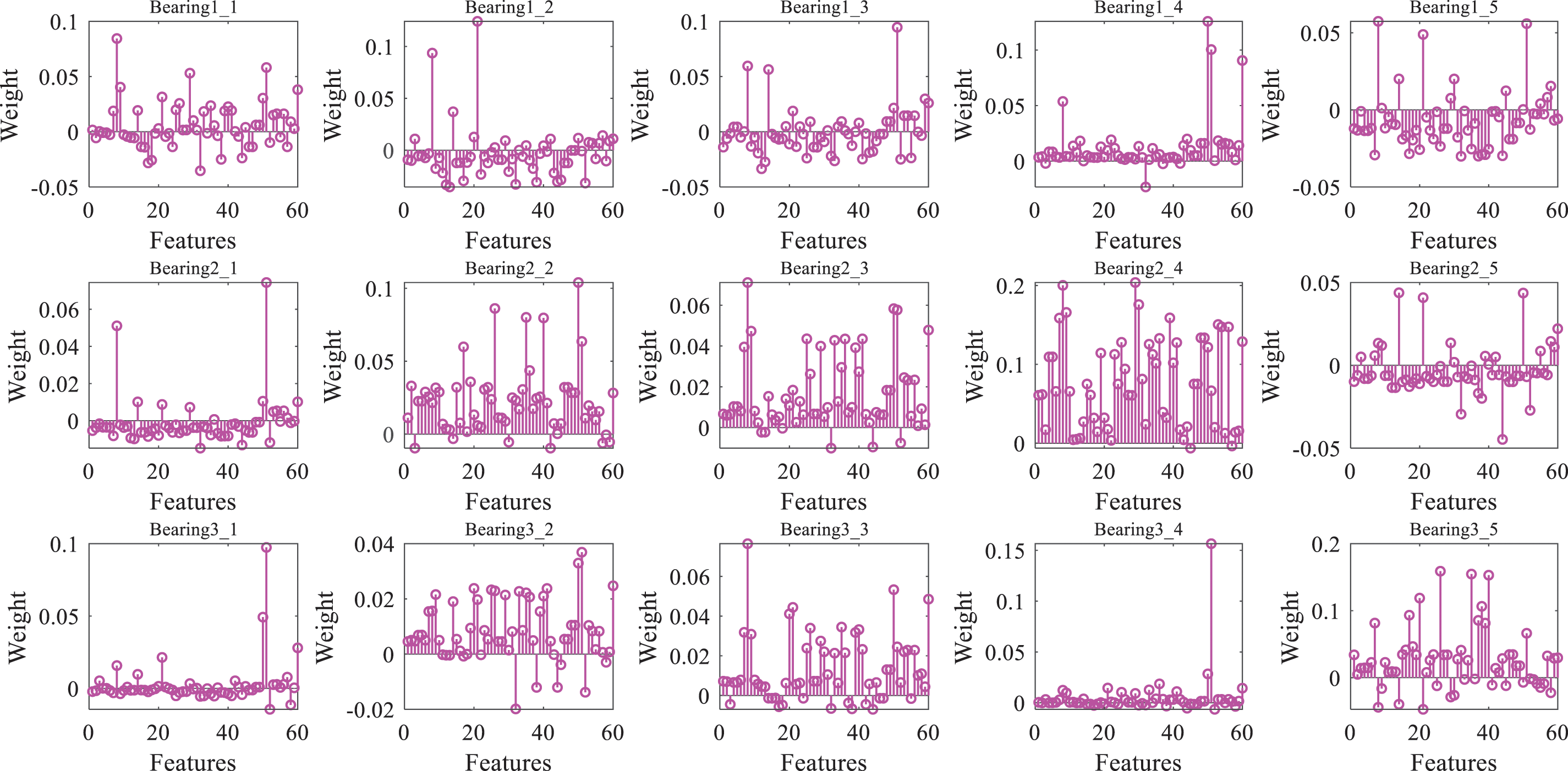
Figure 5: Weights for the sixty features obtained by the RRelifF algorithm
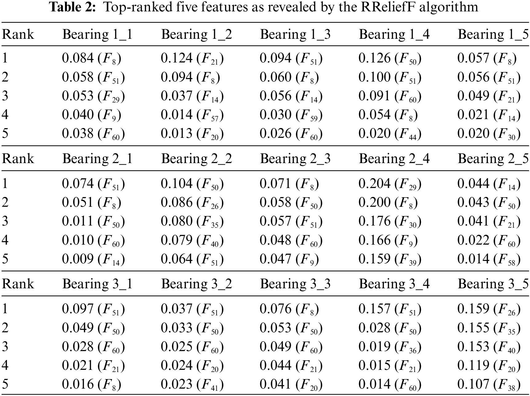
The weight scores of the top 5 features from the ranking over fifteen different bearings are listed in Table 2. Based on the theory of the RRelifF algorithm, the large and sensitive features of the target index can be identified in terms of the weight scores. In other words, the quality of features with strong dependencies can be distinguished with the feature selection technique. As is quantitatively tabulated in Table 2, the top five features are different for the bearings on the different operation conditions. The weight score of the features varies with the different bearings. Hence, the sensitive features can be selected by ranking the weight scores. In this study, ten features are bagged to form the sub-feature set, and the appropriate feature set is selected to ensure the best performance of the prediction model.
The bearing data are fed into the proposed regression model to establish an RUL predictive model. The cross-validation approach is employed to validate the robustness of the prediction model as follows. The entire bearing datasets are divided into three groups according to three operating conditions (i.e., 12, 11, and 10 kN). One bearing dataset is selected as the training set, while the remaining datasets are used as testing sets. This procedure is repeated until all bearing datasets are used, as depicted in Fig. 6. Implementing this method could help determine the best scale of the training datasets for the test bearing. Five different cases are considered in this experiment based on the XJTU-SY bearing datasets. In this technique, five iterations are performed. The data set is divided into five sections in each iteration. One bearing set is utilized as the training data to build the prediction model, and the remaining four bearings are used as the test set. This approach aims to construct a predictive model with an appropriate training data sample size. The cross-validation approach is applied to validate the effectiveness and robustness of the prediction model.
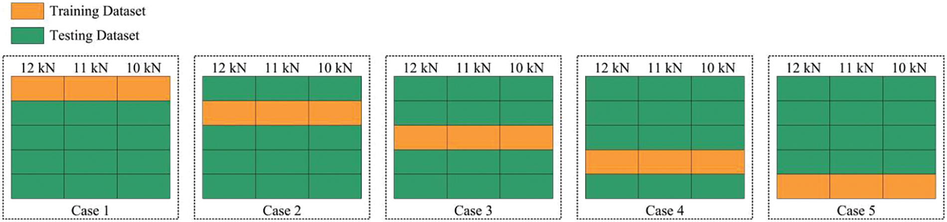
Figure 6: Schematic of the cross-validation method
Table 1 lists the comprehensive operating conditions of the 15 rolling element bearings. It indicates the five Bearing 1_x (Bearing 1_1, Bearing 1_2, Bearing 1_3, Bearing 1_4, and Bearing 1_5) are operated under the same conditions with 12 kN radial force and 2,100 rpm rotating speed. Hence, these five bearings are the same to some extent. It can use the data of Bearing 1_x as the sub-datasets each other when the RUL prediction model of Bearing 1_x is built. In addition, this is the same as the Bearing 2_x and Bearing 3_x. However, Bearing 2_x and Bearing 3_x are operated under Condition 2 and 3, respectively. Thus, the Bearing 2_x and Bearing 3_x can not be used while training the Bearing 1_x. Eventually, there are only 5 cases in the cross-validation method, as shown in Fig. 6.
To select the appropriate feature set to ensure the best performance of the prediction model, the several numbers of features sorted by the RReliefF algorithm, namely, 10, 20, 30, 40, 50, and 60, were considered in the experiment for comparison. Fig. 7 illustrates the performance of the established prediction model for the various feature sets. It indicates that the performance of the proposed prediction model varies for each feature set. When features = 20, i.e., retaining the top 20 features according to the modeling procedure, both the training and test data are formed with 20 input features. The training dataset and input features are selected while the best performance is achieved, i.e., the R2 score is the largest among the cross-validation experiments. In Case 1, the data for the first bearing under the three operation conditions (Bearing 1_1, Bearing 2_1, and Bearing 3_1) are used as the training data. The predicted results of the test bearings vary. In other words, the R2 scores peak at different points. For example, the R2 score is the largest at the 20 input feature points for the test data set of Bearing 2_3. This suggests that when Bearing 2_1 was used as the training data, the predicted result of Bearing 2_3 was the best among all four test sets. In this case, the optimal training set can be obtained for the other four test sets. Cross-validation experiments were conducted based on the five cases to find the optimal training set for all the bearings. From the fifteen subgraphs depicted in Fig. 7, the optimal training set for the bearings is obtained through cross-validation. Taking Bearing 1_3 dataset as an example, the remaining four datasets (Bearing 1_1, Bearing 1_2, Bearing 1_4, and Bearing 1_5) are utilized as training data. Accordingly, the ELM is utilized to predict the RUL and the R2 score is calculated for each pair (C, L) in the grid space. The training set and pair (C, L) with the largest value of the R2 were selected, and these selected parameters were applied to train the entire training data to obtain the ultimate RUL predictor.

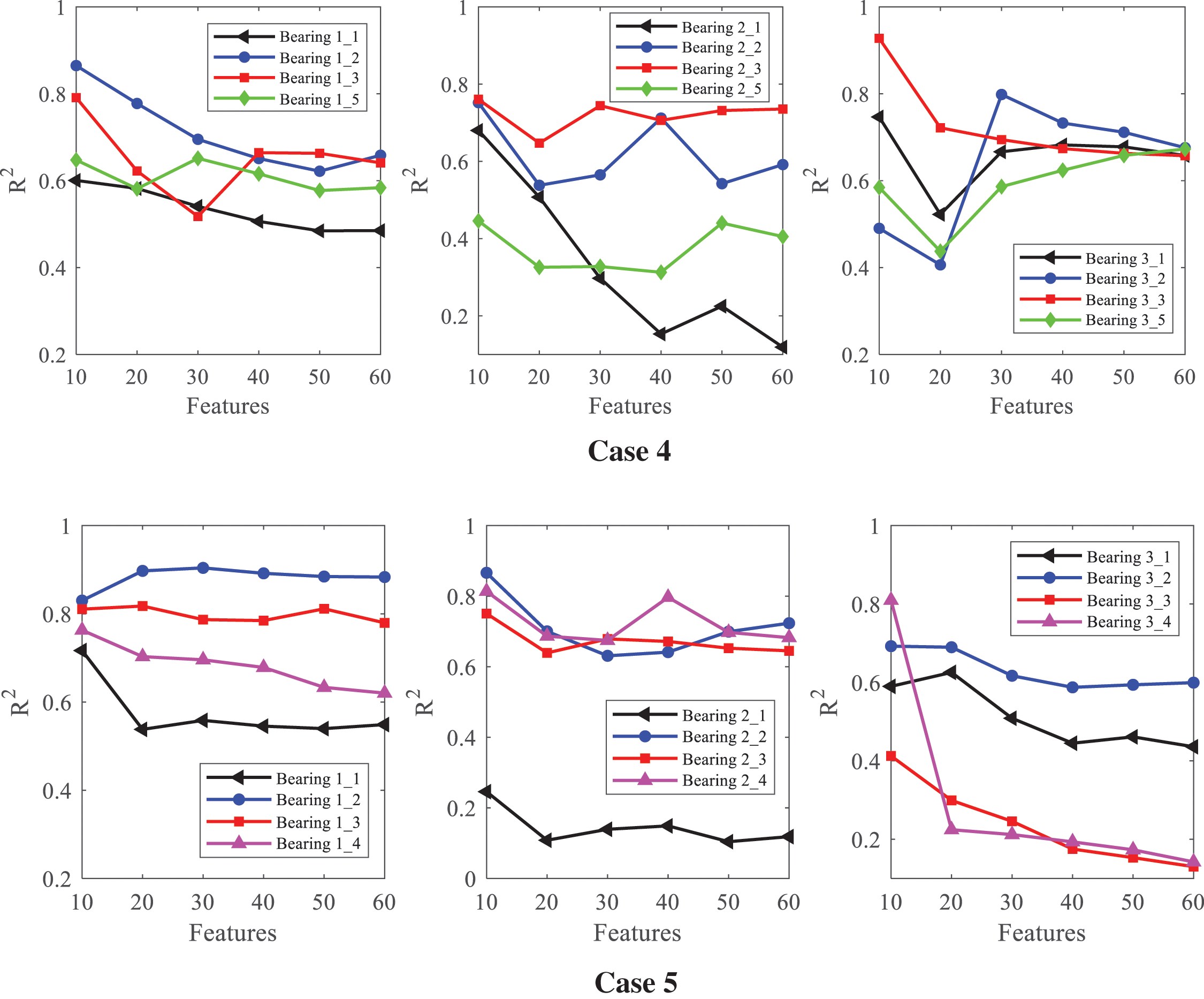
Figure 7: Performance of the prediction model for different feature sets
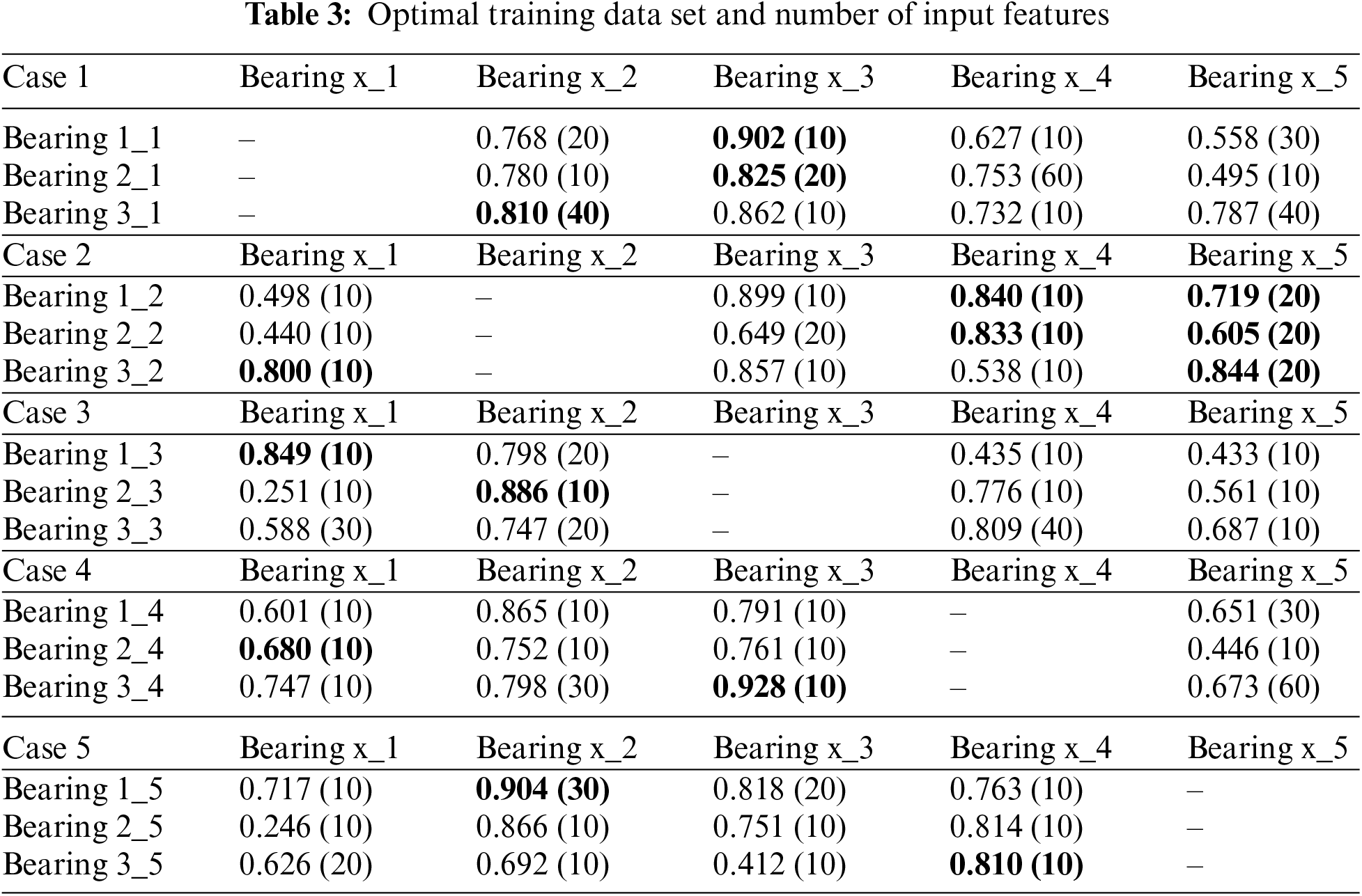
The predictive results of the cross-validation method are shown in Fig. 7. To determine the optimal training dataset and the number of input features, the model’s performance with the cross-validation method is listed in Table 3. The first column denotes the bearing used as the training set, and the row in the different cases denotes the four other bearings used as the test set. The value is the largest R2 with the best sub-feature set within parentheses based on the rank sequence {10, 20, ..., 60} extracted using the RReliefF algorithm. The best parameters of the model are obtained with the largest R2 in the same column and the same row in different cases. For example, Bearing 1_1 used as the test set, and the best training set is searched in the first column (Bearing x_1) within Case 2 to Case 5 in the first row. Four different values can be selected as 0.498 (10), 0.849 (10), 0.601 (10), and 0.717 (10). Obviously, 0.849 (10) reaches the largest R2 among the four cases. Therefore, we get the Bearing 1_3 as the training set for the Bearing 1_1 as the test set and the number of input features comes to 10 in the parentheses.
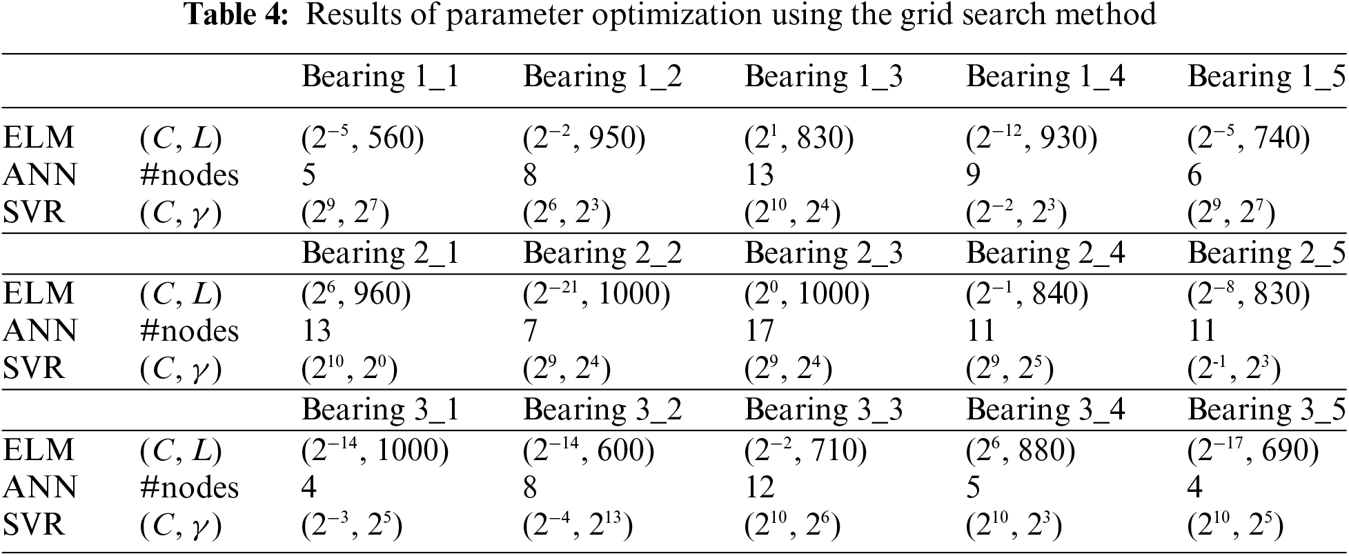
The proposed ELM model used for RUL prediction of the bearings was validated by reducing the input feature dimensions and optimizing the parameters. The optimal values of the model parameters are presented in Table 4. The parameters of the SVR and ANN algorithms are also displayed in Table 4. The predictive results of the three models can be obtained using these parameters.
The performances of the three models were evaluated and compared to the metrics mentioned above (MAE, RMSE, R2) to test whether the hybrid predictive model outperforms the other two models. Consequently, the comparison results are listed in Tables 5–7. The smaller the results of MAE and RMSE, the closer the experimental results obtained by the model are to the real values. R2 is independent of scale because it is dependent on correlation; thus, it is of greater significance for evaluating predictive models. The proposed ELM model achieves 0.65–0.96 regarding R2 values, which states that the predictions are reasonable. Although the proposed predictive method cannot be highly accurate for all bearings, it is still considered to significantly assist mechanical manufacturing enterprises in understanding the degree of degradation process of mechanical equipment during the design stage.
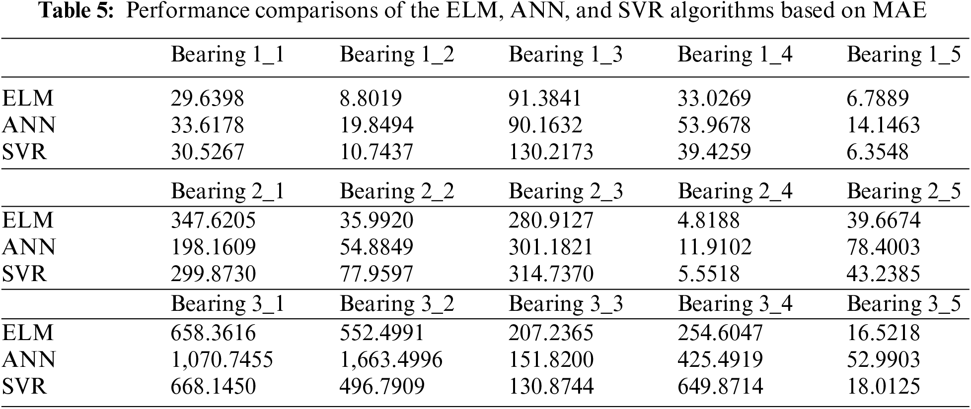
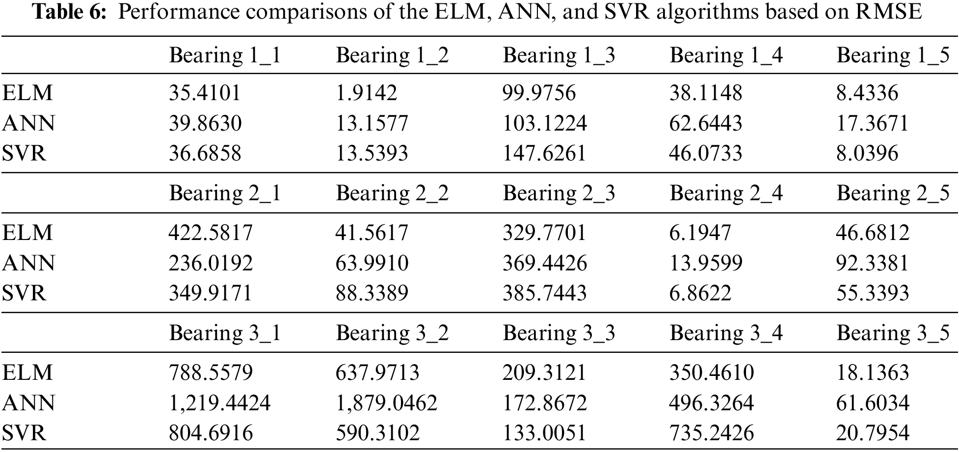
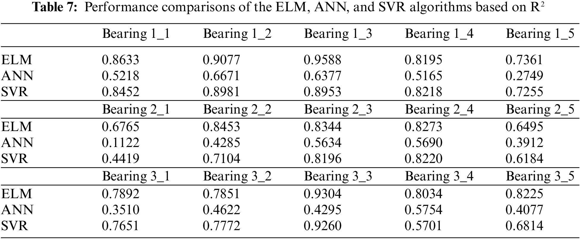
Tables 5–7 display the predicted results of the ELM, ANN, and SVR on the prediction of RUL for bearings. Tables 5 and 6 compare the three regression models to MAE and RMSE. The established ELM model performs better than the other two machine learning algorithms because it yields the smallest MAE and RMSE in most cases. The measurement index R2 values of the predictive models for the RUL of bearings are listed in Table 7. R2 is higher than 0.8 for two-thirds of the fifteen bearings. In most cases, the proposed hybrid approach performs better than ANN and SVR models. These tables indicate that the proposed ELM model outperforms the other two traditional machine learning methods regarding MAE, RMSE, and R2. The ELM exhibits the strongest generalization ability among all algorithms tested. In most cases, the generalization ability of the SVR is poorer than that of ELM but better than that of ANN. Because the hybrid predictive model yielded the minimum MAE and RMSE values and the largest R2 scores in this study, we can conclude that the performance of the established ELM method combined with the RReliefF feature selection algorithm is much better than that of the other two machine learning approaches regarding the RUL of bearings.
This study proposes a bearing RUL prediction model to identify the features associated with RUL by employing the RReliefF algorithm. Accordingly, sixty time-domain features are reconstructed, and the RReliefF algorithm is employed to reduce the dimensionality of the candidate input features. The optimal input feature set is obtained to interpret the complex nonlinear relationship between the input attributes and the output feature (i.e., RUL of bearings). A cross-validation approach is utilized to examine the significance of the training data set in predicting RUL for different bearings. The optimal training dataset and the highly relevant features are fed to the ELM method to construct a predictive model for the RUL of roll element bearings.
The main contributions of this research can be summarized as follows. First, the highly relevant variables are extracted from the sixty candidate time-domain features to estimate the bearings’ RUL. With fewer and more relevant features, the proposed model can more accurately predict the RUL of rolling element bearings. Second, the cross-validation approach is employed to confirm the optimal training bearing set for different testing bearing sets. Third, the predictive results obtained using the proposed hybrid model are compared to those obtained using the other machine learning methods (ANN and SVR). The comparative tested results indicated that the hybrid predictive method is the best estimator of the three models for predicting the RUL of bearings because it yielded the smallest errors. Consequently, the proposed prediction model can more accurately predict the RUL of bearings.
The established prediction model for the RUL of bearings can be utilized to reliably evaluate the operating process of bearings in rotating machines. Therefore, it can be applied to help machinery enterprises understand the sustainability level of their equipment at the design stage. Eventually, an accurate model for the RUL of bearings can act as a guideline for the early stage of the equipment design process to guarantee the security and reliability of devices, thus contributing to increasing the productive efficiency in the construction industry.
Acknowledgement: The authors would like to express their sincere gratitude to the anonymous referees for their invaluable and constructive comments, which led to a great deal of improvement in the original manuscript. The authors are grateful to the Editor-in-Chief and the Associate Editors for their professional suggestions and kind encouragement.
Funding Statement: This research is supported by the Anhui Provincial Key Research and Development Project (202104a07020005), the University Synergy Innovation Program of Anhui Province (GXXT-2022-019), the Institute of Energy, Hefei Comprehensive National Science Center under Grant No. 21KZS217, and Scientific Research Foundation for High-Level Talents of Anhui University of Science and Technology (13210024).
Author Contributions: The specific author contributions to the paper are stated as follows: study conception and design: S. H. Wang, T. B. Ma, and K. Yang; data collection: X. Kang; analysis and interpretation of results: S. H. Wang, C. Wang, and X. He; draft manuscript preparation: S. H. Wang, and X. Kang. All authors have reviewed the results and approved the final version of the manuscript.
Availability of Data and Materials: Publicly available datasets [31] were analyzed in this study.
Conflicts of Interest: The authors declare that they have no conflicts of interest to report regarding the present study.
Supplementary Materials: The supplementary material is available online at https://doi.org/10.32604/cmes.2024.049281.
References
1. Nandi S, Toliyat HA, Li X. Condition monitoring and fault diagnosis of electrical motors—a review. IEEE Trans Energy Conver. 2005;20(4):719–29. doi:10.1109/TEC.2005.847955. [Google Scholar] [CrossRef]
2. Han Y, Song YH. Condition monitoring techniques for electrical equipment—a literature survey. IEEE Trans Power Deliv. 2003;18(1):4–13. doi:10.1109/TPWRD.2002.801425. [Google Scholar] [CrossRef]
3. Zhang XL, Han P, Xu L, Zhang F, Wang YP, Gao L. Research on bearing fault diagnosis of wind turbine gearbox based on 1DCNN-PSO-SVM. IEEE Access. 2020;8:192248–58. doi:10.1109/ACCESS.2020.3032719. [Google Scholar] [CrossRef]
4. Mi JH, Liu LL, Zhuang YH, Bai LB, Li YF. A synthetic feature processing method for remaining useful life prediction of rolling bearings. IEEE Trans Reliab. 2023;72(1):125–36. doi:10.1109/TR.2022.3192526. [Google Scholar] [CrossRef]
5. Aye SA, Heyns PS. An integrated Gaussian process regression for prediction of remaining useful life of slow speed bearings based on acoustic emission. Mech Syst Signal Pr. 2017;84:485–98. doi:10.1016/j.ymssp.2016.07.039. [Google Scholar] [CrossRef]
6. Liao HT, Zhao WB, Guo HR. Predicting remaining useful life of an individual unit using proportional hazards model and logistic regression model. In: Proceeding of the Annual Reliability and Maintainability Symposium, 2006 Jan 23–26; New York, USA, IEEE Press. p. 127–32. doi:10.1109/RAMS.2006.1677362. [Google Scholar] [CrossRef]
7. Liao LX. Discovering prognostic features using genetic programming in remaining useful life prediction. IEEE Trans Ind Electron. 2014;61(5):2464–72. doi:10.1109/TIE.2013.2270212. [Google Scholar] [CrossRef]
8. Li NP, Lei YG, Lin J, Ding SX. An improved exponential model for predicting remaining useful life of rolling element bearings. IEEE Trans Ind Electron. 2015;62(12):7762–73. doi:10.1109/TIE.2015.2455055. [Google Scholar] [CrossRef]
9. Jantunen E, Hooghoudt JO, Yi Y, McKay M. Predicting the remaining useful life of rolling element bearings. In: 2018 IEEE International Conference on Industrial Technology, 2018 Feb 20–22; Lyon, France, IEEE Press. p. 2035–40. doi:10.1007/s13042-023-01807-8. [Google Scholar] [CrossRef]
10. Lei YG, Li NP, Jia F, Lin J, Xing SB. A nonlinear degradation model based method for remaining useful life prediction of rolling element bearings. In: IEEE 2015 Prognostics and System Health Management Conference, 2015 Oct 21–23; Beijing, China, IEEE Press. p. 1–8. doi:10.1109/PHM.2015.7380036. [Google Scholar] [CrossRef]
11. Kumar PS, Kumaraswamidhas LA, Laha SK. Bearing degradation assessment and remaining useful life estimation based on Kullback-Leibler divergence and Gaussian processes regression. Measurement. 2021;174:108948. doi:10.1016/j.measurement.2020.108948. [Google Scholar] [CrossRef]
12. Teng W, Han C, Hu YK, Cheng X, Song L, Liu YB. A robust model-based approach for bearing remaining useful life prognosis in wind turbines. IEEE Access. 2020;8:47133–43. doi:10.1109/ACCESS.2020.2978301. [Google Scholar] [CrossRef]
13. Lei YG, Li NP, Gontarz S, Lin J, Radkowski S, Dybala J. A model-based method for remaining useful life prediction of machinery. IEEE Trans Reliab. 2016;65(3):1314–26. doi:10.1109/TR.2016.2570568. [Google Scholar] [CrossRef]
14. Pan DH, Liu JB, Cao JD. Remaining useful life estimation using an inverse Gaussian degradation model. Neurocomputing. 2016;185:64–72. doi:10.1016/j.neucom.2015.12.041. [Google Scholar] [CrossRef]
15. Wang G, Xiang JW. Remain useful life prediction of rolling bearings based on exponential model optimized by gradient method. Measurement. 2021;176:109161. doi:10.1016/j.measurement.2021.109161. [Google Scholar] [CrossRef]
16. Meng Z, Xu B, Cao LX, Fan FJ, Li JM. A novel convolution network based on temporal attention fusion mechanism for remaining useful life prediction of rolling bearings. IEEE Sens J. 2023;23(4):3990–9. doi:10.1109/JSEN.2023.3234980. [Google Scholar] [CrossRef]
17. Zhu GP, Zhu ZN, Xiang L, Hu AJ, Xu YG. Prediction of bearing remaining useful life based on DACN-ConvLSTM model. Measurement. 2023;211:112600. doi:10.1016/j.measurement.2023.112600. [Google Scholar] [CrossRef]
18. Yang JS, Peng YZ, Xie JS, Wang PX. Remaining useful life prediction method for bearings based on LSTM with uncertainty quantification. Sensors. 2022;22:4549. doi:10.3390/s22124549. [Google Scholar] [CrossRef]
19. Wang YP, Wang JB, Zhang S, Xu D, Ge JH. Remaining useful life prediction model for rolling bearings based on MFPE-MACNN. Entropy. 2022;24:905. doi:10.3390/e24070905. [Google Scholar] [CrossRef]
20. Jiang GJ, Yang JS, Cheng TC, Sun HH. Remaining useful life prediction of rolling bearings based on bayesian neural network and uncertainty quantification. Qual Reliab Eng Int. 2023;39(5):1756–74. doi:10.1002/qre.3308. [Google Scholar] [CrossRef]
21. Li JH, Wang ZH, Liu XQ, Feng ZJ. Remaining useful life prediction of rolling bearings using GRU-DeepAR with adaptive failure threshold. Sensors. 2023;23:1144. doi:10.3390/s23031144. [Google Scholar] [CrossRef]
22. Guo RX, Gong B. Research on remaining useful life of rolling bearings using EWT-DI-ALSTM. Meas Sci Technol. 2022;33:095104. doi:10.1088/1361-6501/ac6ec9. [Google Scholar] [CrossRef]
23. Zhang R, Zeng ZQ, Li YF, Liu JH, Wang ZJ. Research on remaining useful life prediction method of rolling bearing based on digital twin. Entropy. 2022;24:1578. doi:10.3390/e24111578. [Google Scholar] [CrossRef]
24. Wang Y, Ding H, Sun XC. Residual life prediction of bearings based on SENet-TCN and transfer learning. IEEE Access. 2022;10:123007–19. doi:10.1109/ACCESS.2022.3223387. [Google Scholar] [CrossRef]
25. Du XJ, Jia WC, Yu P, Shi YK, Gong B. Rul prediction based on GAM-CNN for rotating machinery. J Braz Soc Mech Sci. 2023;45:142. doi:10.1007/s40430-023-04062-8. [Google Scholar] [CrossRef]
26. Zou YS, Zhao SJ, Liu YZ, Li ZX, Song XX, Ding GF. The transfer prediction method of bearing remain use life based on dynamic benchmark. IEEE Trans Instrum Meas. 2021;70:2516211. doi:10.1109/TIM.2021.3121469. [Google Scholar] [CrossRef]
27. Du WL, Hou XK, Wang HC. Time-varying degradation model for remaining useful life prediction of rolling bearings under variable rotational speed. Appl Sci. 2022;12:4044. [Google Scholar]
28. Jin XH, Que ZJ, Sun Y, Guo YJ, Qiao W. A data-driven approach for bearing fault prognostics. IEEE Trans Ind Appl. 2019;55(4):3394–401. doi:10.1109/TIA.2019.2907666. [Google Scholar] [CrossRef]
29. Pan ZZ, Meng Z, Chen ZJ, Gao WQ, Shi Y. A two-stage method based on extreme learning machine for predicting the remaining useful life of rolling-element bearings. Mech Syst Signal Pr. 2020;144:106899. doi:10.1016/j.ymssp.2020.106899. [Google Scholar] [CrossRef]
30. Kuo PH, Tseng TC, Luan PC, Yau HT. Dense-structured network based bearing remaining useful life prediction system. Comp Model Eng. 2022;133(1):133–51. doi:10.32604/cmes.2022.020350. [Google Scholar] [CrossRef]
31. Wang B, Lei YG, Li NP, Li NB. A hybrid prognostics approach for estimating remaining useful life of rolling element bearings. IEEE Trans Reliab. 2018;69(1):401–12. doi:10.1109/TR.2018.2882682. [Google Scholar] [CrossRef]
32. Robnik-Šikonja M, Kononenko I. Theoretical and empirical analysis of ReliefF and RReliefF. Mach Learn. 2003;53:23–69. doi:10.1023/A:1025667309714. [Google Scholar] [CrossRef]
33. Islam T, Srivastava PK, Dai Q, Gupta M, Zhuo L. Rain rate retrieval algorithm for conical-scanning microwave imagers aided by random forest, RReliefF, and multivariate adaptive regression splines (RAMARS). IEEE Sens J. 2015;15(4):2186–93. doi:10.1023/A:1025667309714. [Google Scholar] [CrossRef]
34. Urbanowicz RJ, Olson RS, Schmitt P, Meeker M, Moore JH. Benchmarking relief-based feature selection methods for bioinformatics data mining. J Biomed Inform. 2018;85:168–88. doi:10.1016/j.jbi.2018.07.015. [Google Scholar] [CrossRef]
35. Son H, Kim CM, Kim CW, Kang Y. Prediction of government-owned building energy consumption based on an RReliefF and support vector machine model. J Civ Eng Manag. 2015;21(6):748–60. doi:10.3846/13923730.2014.893908. [Google Scholar] [CrossRef]
36. Huang GB, Zhu QY, Siew CK. Extreme learning machine: theory and applications. Neurocomputing. 2006;70:489–501. doi:10.1016/j.neucom.2005.12.126. [Google Scholar] [CrossRef]
37. Huang GB, Wang DH, Lan Y. Extreme learning machines: a survey. Int J Mach Learn Cyb. 2011;2:107–22. doi:10.1007/s13042-011-0019-y. [Google Scholar] [CrossRef]
38. Roul RK, Asthana SR, Kumar G. Study on suitability and importance of multilayer extreme learning machine for classification of text data. Soft Comput. 2017;21(15):4239–56. doi:10.1007/s00500-016-2189-8. [Google Scholar] [CrossRef]
39. Chong LY, Ong TS, Teoh ABJ. Feature fusions for 2.5D face recognition in random maxout extreme learning aachine. Appl Soft Comput. 2019;75:358–72. doi:10.1016/j.asoc.2018.11.024. [Google Scholar] [CrossRef]
40. Liang NY, Huang GB, Saratchandran P, Sundararajan N. A fast and accurate online sequential learning algorithm for feedforward networks. IEEE Trans Neural Netw. 2006;17(6):1411–23. doi:10.1109/TNN.2006.880583. [Google Scholar] [CrossRef]
41. Hsu CW, Chang CC, Lin CJ. A practical guide to support vector classification. BJU Int. 2018;101(1):1396–400. [Google Scholar]
42. Fan XH, Li Y, Chen XL. Prediction of iron ore sintering characters on the basis of regression analysis and artificial neural network. Energy Proc. 2012;16:769–76. doi:10.1016/j.egypro.2012.01.124. [Google Scholar] [CrossRef]
43. Li Y, Huang X, Zhao C, Ding P. Stochastic fractal search-optimized multi-support vector regression for remaining useful life prediction of bearings. J Braz Soc Mech Sci. 2021;43(9):414. doi:10.1007/s40430-021-03138-7. [Google Scholar] [CrossRef]
Cite This Article
 Copyright © 2024 The Author(s). Published by Tech Science Press.
This work is licensed under a Creative Commons Attribution 4.0 International License , which permits unrestricted use, distribution, and reproduction in any medium, provided the original work is properly cited.
 Downloads
 Citation Tools