Abnormal State Detection in Lithium-ion Battery Using Dynamic Frequency Memory and Correlation Attention LSTM Autoencoder

Nomenclature

1  Introduction

As the electrical systems become increasingly intricate and distributed energy sees broader implementation, Virtual Power Plants (VPP) have been developed. These plants consolidate multiple energy resources, including wind and solar, facilitating centralized control and management. In this context, Lithium-ion batteries (LiBs), with their superior efficiency and energy density, have become an essential component within VPPs. These batteries provide important energy buffering and modulation capabilities for VPPs. For instance, V2G (Vehicle-to-Grid) technology enables electric vehicles (EVs) to act as distributed energy storage devices, selling electricity back to the grid during peak usage times, thereby ensuring the stable operation of the power system. Compared to traditional fossil fuel power generation, EVs cause less pollution in terms of emissions. In addition, Battery Replacement Stations can provide quick battery replacement for EVs. These stations allow EV owners to replace a depleted battery with a fully charged one in minutes, significantly reducing the time spent waiting for a recharge. However, during the use of LiBs in EVs, various abnormal states, such as overcharging, over-discharging, and internal short-circuiting, may occur. These abnormal states not only affect battery performance and lifetime, but also reduce the transmission efficiency of EVs when delivering power to the grid, thus posing a threat to the stability of the VPP system. Therefore, it is essential to accurately and timely detect the abnormal state of LiB [1,2].

The parameters in the charging and discharging process of LiBs are primarily obtained by measuring the battery’s voltage, current, and temperature. LiBs used in EVs come in various structures, including cylindrical, prismatic, and pouch types. The diversity in LiB structures demands greater adaptability in traditional fault detection methods, as performance characteristics and management requirements vary significantly across different applications [3]. In addition, one of the critical challenges in LiB management is to address inhomogeneities within individual cells and variations between cells. These inconsistencies may originate from the manufacturing process and charging and discharging cycles. For example, during the manufacturing process, a cell with a slightly thicker cathode coating may have a higher capacity but also a higher internal resistance, affecting its performance and heat generation during charging and discharging. As the number of charging and discharging cycles increases, the electrolyte and active materials continually degrade, ultimately decreasing the battery’s capacity and efficiency [4].

Conventional Battery Management Systems (BMS) and statistical approaches such as Autoregressive Integrated Moving Average (ARIMA) provide fundamental monitoring capabilities [5], such as tracking parameters like voltage, current, and temperature. These often only reveal the superficial state of the battery and might fail to detect more complex internal abnormal states. For example, internal pressurization of the battery leads to delamination and thus failure of the battery [6–8]. LiB fault diagnosis algorithms that utilize battery models, faults are detected by generating and analyzing residuals based on the models. This includes state estimation, parameter estimation, parity checks, and structural analysis. These methods focus on the physical characteristics and working principles of batteries. For different battery types or operating conditions, continuous adjustments and optimizations of the models may be necessary [9]. As shown in Fig. 1, the parameters of LiBs during charging are complex and inconsistent, with certain abnormal samples closely resembling normal ones, making it challenging to identify irregular states through basic features alone. To achieve more accurate and timely detection of abnormal states, as well as to overcome the challenges of acquiring abnormal samples and the high cost of data labeling, researchers have begun to explore unsupervised machine learning methods. Traditional unsupervised machine learning methods for time series abnormal state detection include One-Class Support Vector Machine (OC-SVM) [10], Isolation Forest (IF) [11], and Principal Component Analysis (PCA) [12], which typically do not require stringent assumptions about the data distribution and can handle complex data patterns. Despite the numerous successes of conventional machine learning approaches in abnormal state detection, they are typically sensitive to the choice of parameters, incur high computational costs, and might struggle with handling exceedingly complex, high-dimensional, or non-linear data structures.

Figure 1: Visualization of normal and abnormal charging processes of some electric vehicle Lithium-ion batteries

Recently, unsupervised deep learning abnormal state detection algorithms based on autoencoders (AE) have garnered widespread attention [13,14]. AE can automatically learn high-level features from normal data and capture complex and nonlinear patterns in the data. Generating significant reconstruction errors when encountering abnormal samples, thus detecting abnormal states [15]. However, the behavior of batteries is highly time-correlated, changing according to the current state of the battery (such as charging status, temperature, or electrochemical state), meaning that the same absolute measurements can indicate different things under different states. For instance, a rapid increase in current may be normal during the early stages of charging, but such an increase nearing full charge could be indicative of an abnormal state [16]. Such temporal correlations are easily neglected by AE. Furthermore, battery behavior is also frequency-dependent. These dependencies are conspicuous in new batteries but may start to diverge subtly with battery aging. For example, aged batteries may exhibit irregular frequency characteristics in thermal cycles at the same working temperature due to decreased thermal management capabilities [17]. AE is also not very sensitive to frequency correlations. Lastly, given the high complexity of LiB data, AE typically requires the setting of numerous parameters, which results in an overly strong generalization capability, effectively reconstructing some abnormal samples too well [18].

To address the challenges mentioned, we propose a novel unsupervised abnormal state detection model for LiB time series: DFMCA-LSTM-AE (Long Short-Term Memory Autoencoder with Dynamic Frequency Memory and Correlation Attention). We primarily enhance the conventional AE through two components: the Dynamic Frequency Memory and Correlation Attention mechanism (DFMCA) and the Long Short-Term Memory network (LSTM) [19]. DFMCA is a core component of the DFMCA-LSTM-AE model, merging the benefits of dynamic convolution and fast Fourier transform to enhance the model’s ability to capture frequency correlations. Dynamic convolution can adjust its kernel size adaptively, thus more flexibly capturing local and global features in the time series [20]. The model can detect frequency patterns of battery behavior across various time scales by weighting the fast Fourier transform after multi-scale dynamic convolution. Notably, all fast Fourier transforms within the DFMCA are followed by a memory module that can remember the frequency characteristics of normal samples during the training phase and reconstruct the input samples based on the memory items to assist in distinguishing between normal and abnormal states. The LSTM layer follows closely after the DFMCA. Its role is to receive frequency correlation features enhanced by the attention module and further analyze how these features evolve. The internal gate-controlled mechanism of the LSTM proficiently filters and retains important temporal points, ignoring irrelevant data, thus allowing the LSTM layer to detect subtle shifts in battery status. The principal contributions of this paper are as follows:

•   We proposed the DFMCA-LSTM-AE abnormal state detection model for the EV LiB time series. This model is end-to-end and unsupervised.

•   Dynamic Frequency Memory and Correlation Attention mechanism and LSTM layer are introduced, effectively capturing battery behavior’s frequency and temporal correlations.

•   A memory module is incorporated after the fast Fourier transform to remember features of normal samples, reducing the model’s overgeneralization.

•   Experiments on a real-world LiB dataset demonstrate the effectiveness of DFMCA-LSTM-AE, with its performance significantly surpassing other representative models and the state of art model.

2  Related Works

Time series abnormal state detection is an active research topic that has been extensively studied. The related work involved in this paper includes unsupervised time series abnormal state detection and memory networks.

2.1 Unsupervised Time Series Abnormal State Detection

An abnormal state refers to values that deviate significantly from observations. Methods for detecting abnormal states in time series can be divided into statistical methods, machine learning methods, and deep learning methods. Statistical methods include algorithms such as the standard deviation method (Z-Score) [21], Autoregressive Integrated Moving Average (ARIMA) [22], and Exponential Smoothing [23]. Statistical methods often require specific assumptions like data distribution, which may not always hold in practical applications. Machine learning techniques involve algorithms like k-means [24], OC-SVM [10], IF [11], and PCA [12]. However, most machine learning models cannot learn directly from raw time series data, often necessitating initial feature engineering and meticulous parameter selection and tuning to identify features significant for detecting abnormal states. Deep learning methods include the use of Autoencoders, Variational Autoencoders (VAE) [25], LSTM [19], and Generative Adversarial Network (GAN)-based approaches [26]. In general, deep learning can learn high-level data representations to capture complex patterns and relationships effectively. Additionally, deep learning allows for direct training of models from raw data to outcomes, significantly reducing the need for data preprocessing and feature engineering.

Furthermore, time series abnormal state detection methods based on deep learning can be divided into two types. The first type generates predicted data based on historical data and compares it with the input sample to detect abnormal states. Wu et al. utilized LSTM to predict time series data, followed by applying a naive Bayes model for error evaluation [27]. Meng et al. employed the Transformer for time series forecasting, incorporating an attention mechanism with parallel time step updates and a masking strategy for early abnormal state detection, improving the ability to recognize abnormal states [28]. Nonetheless, these methods are deficient in global observation and can be affected by real-time impacts from other variables, rendering them unsuitable for the dynamically changing data of LiB. The other type is based on models trained on historical data to reconstruct input samples, with the reconstruction results compared with the input samples to detect abnormal states. This method makes better use of global information and is more stable than other methods. Zhang et al. combined Convolutional Neural Networks (CNN) with LSTM to concurrently capture the spatial and temporal characteristics of time series data, embedding this hybrid into the architecture of an autoencoder. By comparing multi-scale data reconstructions, the architecture can effectively identify abnormal patterns [29]. Zhang et al. proposed a Dynamic Autoencoder Model (DyAD) that dynamically encodes LiB data, adding an auxiliary loss to achieve latent space regularization [30].

2.2 Memory Network

In 2014, Weston et al. first introduced a model called Memory Networks [31], which is a memory structure for external information, applicable to many tasks such as question answering and language modeling. Subsequently, Sukhbaatar et al. proposed its end-to-end version, optimizing the training process [32]. Kumar et al. then released an improved version of the memory network known as the Dynamic Memory Network (DMN). This DMN model combines a Recurrent Neural Network (RNN) with an external memory component, first processing the input through the RNN, and then saving the processed results in the memory component [33]. Chang et al. utilized a memory module as a dynamic knowledge base to capture its long-term patterns. Moreover, it is easy to know which parts of the historical data are most frequently referenced by the attributes of the memory module, making the model highly interpretable [34]. Gao et al. proposed a memory-augmented time series autoencoder (TSMAE). A memory module is added between the encoder and the decoder, and each memory item is encoded and recombined based on the similarity of latent representations, encouraging the memory module to extract typical normal patterns of the time series, thus suppressing the model’s generalization ability [35].

3  Methodology

Integrating EVs into smart grid ecosystems brings about complex data streams and interactions, requiring advanced techniques for monitoring and management. To unlock the full potential of this integration, advanced models must be utilized to interpret and act upon the substantial data produced by EVs. The proposed DFMCA-LSTM-AE model’s application context, depicted in Fig. 2, demonstrates how EVs are capable of producing diagnostic data through the Battery Management Systems (BMS) at charging facilities during the charge and discharge cycles. This encompasses a sequence of fluctuating parameters that develop over the course of LiB charge-discharge cycles. Subsequently, this diagnostic information is transmitted to a cloud-based server for further analysis and processing. The trained DFMCA-LSTM-AE is deployed on the cloud server to perform real-time abnormal state detection on the monitoring data, and report to the user if abnormal states are generated when EVs are charging. On the other hand, when EVs discharge to the grid, if too many abnormal states are detected, additional planning is done to utilize other energy sources in the virtual power plant. By situating the DFMCA-LSTM-AE model within the cloud server, we benefit from the computational power and scalability needed to process large datasets in real time. This high-level functionality is crucial for rapidly identifying potential issues and implementing corrective measures within the VPP ecosystem.

Figure 2: Application of DFMCA-LSTM-AE in virtual power plant

3.1 Overview

The proposed DFMCA-LSTM-AE model consists of a Dynamic Frequency Memory and Correlation Attention Mechanism (DFMCA), LSTM layers, and the corresponding encoders and decoders. Fig. 3 shows the input being mapped onto queries (Q), keys (K), and values (V). Q and K are then fed into the Dynamic Fourier Transform Memory Module (DFTM), depicted in Fig. 4. Within the DFTM, inputs pass through one fast Fourier transform (FFT) branch without dynamic convolution. Additionally, they go through two FFT branches that include dynamic convolutions of different sizes. This process allows for the dynamic capture of multi-scale frequency features. The output of each branch is then processed by the memory module, which retrieves the most relevant items in memory based on attention-based addressing weights and outputs them. The six frequency features output by the DFTM are multiplied accordingly to obtain three sets of frequency relevance features, which are then subjected to inverse FFT projection into the time domain. Weighted summation via the attention mechanism. Finally, the largest p values from the features are selected for dynamic information synthesis with V. The output of the DFMCA is then passed through two sets of linear layers and LSTM layers to obtain reconstructed samples. The prediction part is based on the reconstruction error between the input sample and the reconstructed sample, if the reconstruction error is greater than a set threshold then the input sample is considered abnormal, and vice versa for normal sample.

Figure 3: DFMCA-LSTM-AE architecture

Figure 4: Dynamic fourier transform memory module and memory module architectures

3.2 Time-Series Data Preprocessing

Larger numerical values can expand the range of scales, rendering the model insensitive to minor variations in smaller numerical values, which could result in neglecting their crucial properties. Hence, considering the sensor context information under the same timestamp, it is necessary to standardize the raw data for all temporal dimensions.

The raw data D∈ℜn×f×L is a matrix that consists of n samples of time series. The feature number of time points is f. The length of each time series is L, which signifies the data gathered during each sampling cycle. For every data point d, the maximum and minimum values in its corresponding column ∈ℜfare utilized as the parameters for its normalization. The normalized data x is shown in Eq. (1).

x=d−Mincol(d,D)Maxcol(d,D)−Mincol(d,D)(1)

where Mincol(d,D) refers to the minimum value in the column in which d∈D is located. Maxcol(d,D) refers to the maximum value in the column in which d∈D is located.

3.3 Dynamic Fourier Transform Memory Module

3.3.1 Dynamic Convolution

As shown in Fig. 4, when data S∈ℜf×H×L is fed into the DFTM module (with H representing the number of attention mechanism heads), it enters three distinct branches for frequency feature extraction. Data passing through the S1 branch undergoes a direct FFT to extract the overall frequency features of the data. The FFT expression is shown in Eq. (2).

u[k]=∑t=0L−1St⋅e−2πjLkt,k∈{0,1,2,…,L−1}(2)

where u[k] refers to the k-th element of the FFT output frequency domain signal. j is an imaginary unit. St∈ℜf×H denotes the t-th time point of the input S.

The S2 branch is utilized for medium-scale dynamic convolution and FFT to extract frequency features. When data passes through the S2 branch, it first undergoes a 1D dynamic convolution, which can dynamically adjust the convolution kernel’s weights based on the different input time series. This method effectively overcomes the limitations of general convolution in generalizing over data with dynamic changes and poor regularity. Differing from [20], we do not use squeeze-and-excitation [36] to compute kernel attention but instead employ an Efficient Channel Attention Network (ECA-Net) [37], which avoids the computational burden of fully connected layers. Initially, global spatial information is compressed through global average pooling. Subsequently, we use a convolutional layer with a kernel and stride of 1, along with σ (SoftMax), to generate normalized attention weights πg for g convolutional kernels. Notably, the output of ECA-Net is not channel attention but kernel attention. Once the kernel weights are obtained, dynamic convolution kernels are produced following Eq. (3).

WDy=∑i=1gπi⋅Wi(3)

where Wi∈ℜCout×Cin×C represents the i-th, i∈{1,2,…,g} parallel convolution kernel. Cout is the number of output channels, Cin is the number of input channels, and C denotes the number of convolution kernels. πi is the weight of the i-th kernel. The term g denotes the number of parallel convolution kernels, which is 4 in this paper.

After obtaining WDy, convolution is performed on the compressed input x∈ℜCin×L∗, with bias term b∈ℜCout. L∗ is the length of the sequence x under stride C and zero padding. The output y∈ℜCout×L∗ is shown in Eq. (4).

y=x⋅WDy+b(4)

The branch where S3 is located is used for large-scale dynamic convolution and FFT to extract frequency features of the data. Unlike the branch where S2 is located, which has C convolution kernel size for Wi and a stride of C, the branch for S3 uses Wi with C2 convolution kernel size and a stride of C2.

3.3.2 Memory Module

The frequency features transformed by FFT are represented as u∈ℜf×F, where F denotes the length of the frequency feature sequence. The memory M∈ℜN×f consists of N memory items m∈ℜN. The attention addressing vector e∈ℜN is calculated as the inner product of the frequency features with each memory item, aimed at gauging the matching degree between the frequency features and each memory cell. The SoftMax function is applied to the match scores between each memory item and the frequency features to determine similarity distances. The formula associated with the similarity distance related to each memory cell is seen in Eq. (5).

ei=SoftMax(umiT)=exp⁡(umiT)∑j=1Nexp⁡(umjT)(5)

where ei denotes the i-th, i∈{1,2,…,N} attention addressing vector and mi denotes the i-th, i∈{1,2,…,N} memory term.

The higher the value of ei, the greater the similarity of the corresponding addressing vector to the normal sample. Conversely, the lower the value of ei, the lower the similarity. These addressing vectors are then used to reconstruct the frequency feature u^, as shown in Eq. (6).

u^=eM=∑i=1Neimi(6)

Although backpropagation can reduce the sensitivity of addressing vectors with low relevance to the normal samples based on gradient descent, when the number of addressing vectors reaches a certain scale, even those with low sensitivity can reconstruct abnormal samples through linear combination. To address this issue, we employed the addressing adjustment technique proposed by Gong et al. [38], as shown in Eq. (7), which limits the lower bound of addressing vector ei.

e^i=max(ei−λ,0)⋅ei|ei−λ|+ϵ(7)

where λ is a threshold allowing ei values less than λ to become 0, to prevent division by zero, an extremely small positive number ϵ is additionally added.

3.4 Dynamic Frequency Memory and Correlation Attention

Dynamic Frequency Memory and Correlation Attention can perform a correlation calculation on the frequency features captured by the DFTM and associate the frequency correlation with multiple similar subsequences through dynamic information synthesis, thereby indirectly linking the frequency correlation with temporal relationships.

3.4.1 Weighted Feature Fusion

As shown in Fig. 3, qi and ki, i∈{1,2,3}, represent the i-th output of the DFTM module. The correlation of each group of frequency features is calculated through Eq. (8), and an inverse fast Fourier transform (IFFT) is applied, making the dimensionality of frequency correlation the same as that of V∈ℜf×H×L.

Corr((qi,ki),t)=IFFT(qi⋅Conj(ki),t)=1L∑k=0L−1u[k]⋅e2πjLkt(8)

where Corr((qi,ki),t) denotes the correlation between qi and ki at moment t∈{0,1,2,…,L−1}. IFFT(⋅,t) refers to the moment t when the input is transformed by the IFFT. Conj(ki) denotes the conjugate operation on ki. k∈{0,1,2,…,L−1} refers to the index of the frequency component. j is an imaginary unit.

If conventional feature fusion methods are used to add the three sets of frequency correlation together simply, it is equivalent to assuming that the frequency correlation at each scale is equally significant. Although this increases multi-scale information, it still causes certain information redundancy, making it difficult to allocate attention weights reasonably. Therefore, we have incorporated ECA-Net before feature fusion, allowing the model to dynamically assign weights based on each group’s frequency correlation information content.

3.4.2 Dynamic Information Synthesis

The frequency correlation after weighted feature fusion is compressed to obtain AttCorr∈ℜL, where L is the length of the time series V. The largest p values in AttCorr are selected, in this paper p is 4, and then SoftMax is applied to obtain the importance weights on the time dimension, as shown in Eq. (9).

WAttCorri=exp⁡(AttCorr(i))∑j=1Lexp⁡(AttCorrj)(9)

where AttCorr(i) refers to the i-th large value in AttCorr, and WAttCorri refers to the importance weight corresponding to the i-th maximal time index βi, i∈{1,2,3,4}. AttCorrj refers to the j-th in AttCorr.

In a time series V of length L, the time points preceding βi in V are first moved to follow V. Then, they are sequentially multiplied and summed with their respective importance weights, as illustrated in Eq. (10).

Y=∑i=1PMov(V,βi)⋅WAttCorri(10)

where Y∈ℜf×H×L denotes the final output of all DFMCA heads and Mov(⋅) denotes the sequence shift operation. The final output Y∗∈ℜf×L should be the result of averaging the dimensions where the head is located.

3.5 Long Short-Term Memory Network

To account for the temporal relationships before and after each data item in the time series, DFMCA-LSTM-AE incorporates an LSTM layer. LSTM is a special type of RNN, consisting of multiple sequential cells. Unlike RNN, each cell controls the flow of information through three gates, which determine what information is stored, deleted, or outputted. The forget gate ft∈[0,1]H controls how much of the previous time step’s cell state will be retained. The input gate it∈[0,1]H controls how much new information will be stored in the cell state, and Ct~∈[−1,1]H is a candidate value representing new information that may be added to the current state. The cell state Ct∈ℜH is updated through the output of the forget gate and input gate, along with a nonlinear function. The output gate ot∈[0,1]H controls how much of the cell state information will be used as the hidden state ht∈ℜH for this time step. H is the dimension of the hidden state. The computational process of each LSTM cell can be represented as follows:

ft=σ(Wf⋅[ht−1,xt]+bf)(11)

it=σ(Wi⋅[ht−1,xt]+bi)(12)

C~t=tanh⁡(WC⋅[ht−1,xt]+bC)(13)

Ct=ft∗Ct−1+it∗C~t(14)

ot=σ(Wo⋅[ht−1,xt]+bo)(15)

ht=ot∗tanh⁡(Ct)(16)

In the above equation, xt∈ℜL represents the input at the current moment, σ denotes the sigmoid function, which is used to generate an output between 0 and 1, indicating the degree to which the gate is open. The tanh represents the hyperbolic tangent function, with an output range of –1 to 1. W and b are the weight matrix and bias vector, corresponding to the forget gate Wf, bf, the input gate Wi, bi, WC, bC, and the output gate Wo, bo, respectively. ∗ denotes the Hadamard product. [ht−1,xt] indicates the concatenation of the previous hidden state with the current input. Finally, {h1,h2,…,hL} as the output of the encoder is fed into the decoder.

3.6 Encoder and Decoder

The encoder is responsible for extracting the latent representation with attention from the input, while the decoder restores the latent representation to obtain the reconstructed sample. The formulas for the encoder and decoder are seen in Eqs. (17) and (18).

z=fe(x)(17)

x^=fd(z)(18)

where z denotes the potential representation of the output of the input sample x after the encoder fe(⋅). The reconstructed sample x^ is then obtained by the decoder fd(⋅).

3.7 Loss Function

In the training phase, the dataset comprises exclusively normal samples. The training aims for the model to acquire the primary characteristics of normal samples, thereby effectively reconstructing them and generating a specific deviation when dealing with abnormal state samples. Mean squared error (MSE) is employed as the loss function, with the computational formula provided in Eq. (19).

ℒ(x,x^)=1L∑j=1L(xj−x^j)2(19)

where xj is the j-th input time point, x^j is the j-th reconstructed time point, j∈L, and L denotes the number of time points in the time series.

The design of the loss function is crucial as it guides the model during training by quantifying the difference between the reconstructed time series and the original input. The MSE specifically penalizes larger errors more severely, as the errors are squared, and it averages these overall points in the time series to give a single scalar quantity representing the loss. This function encourages the model to minimize the difference between the normal operational data it has learned and any new data it is reconstructing, thus helping to identify anomalies by the deviation in the reconstruction error.

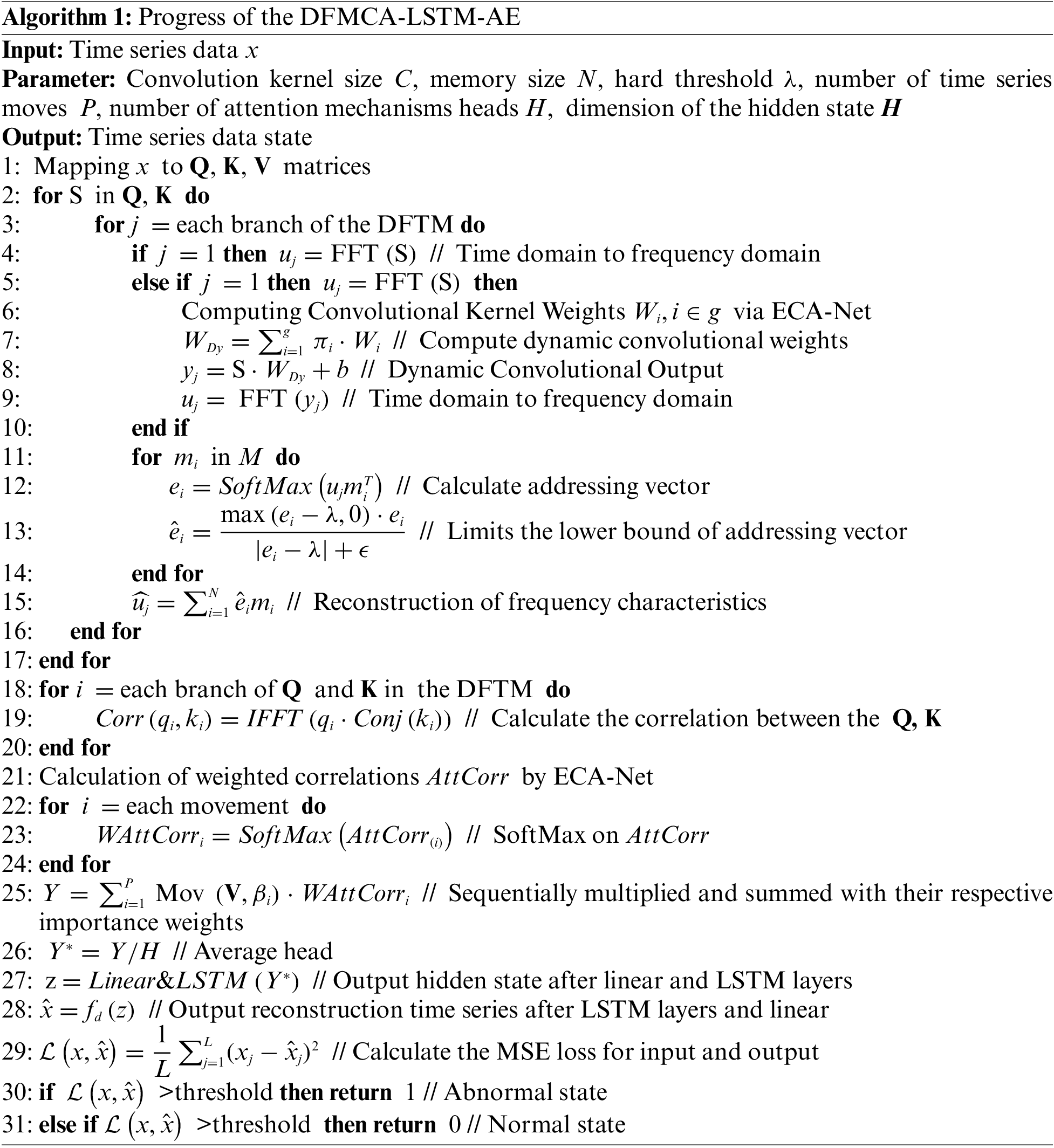
The computational flow of the DFMCA-LSTM-AE is shown in Algorithm 1. Algorithm 1 commences with the mapping of time series data x into matrices Q, K, and V. Subsequently, the first branch of the DFTM applies FFT directly to the input S. The remaining branches produce an output yj after dynamic convolution, upon which FFT is also performed. Secondly, cc, where SoftMax calculates the distance between the frequency feature and each memory item to form an addressing vector ei. This vector is subjected to hard thresholding to refine the addressing combination. New frequency characteristics uj^ are reconstructed by memory items M with the weighted addressing vector. Thirdly, the reconstructed frequencies corresponding to Q and K are correlated to yield Corr(qi,ki). This is then compressed via an ECA-Net to produce AttCorr, which is subsequently refined by SoftMax to obtain WAttCorr. Fourthly, a time lag is applied based on the maximum P values, and these are multiplied by the corresponding AttCorr to produce Y, which, when divided by the number of attention heads, results in Y∗. Fifthly, Y∗ passes through two LSTM layers and two linear layer to reconstruct the time series x^. Finally, the anomaly score ℒ(x,x^) is derived from the MSE loss between x and x^, with anomaly scores exceeding a threshold indicating an abnormal state for x. In contrast, scores below the threshold indicate a normal state.

4  Experimental and Results

4.1 Experimental Setup

4.1.1 Datasets

This article conducts experiments on the real-world EV lithium-ion battery dataset released in [30]. The dataset contains over 690,000 real charging segments from 347 EVs. The number of abnormal state segments accounts for 18.57% of the total. Each charging segment has 128 time points, with an interval of 10 s between each point, comprising 7 features. The visualization of each feature is shown in Fig. 1.

4.1.2 Metrics

The Receiver Operating Characteristic (ROC) curve is a common tool for visualizing the classification performance of binary classification models. It works by arranging all possible classification thresholds, calculating a series of False Positive Rate (FPR) and True Positive Rate (TPR) points, and then plotting them on a chart. The Area Under the ROC Curve (AUC) is often used to measure the classification performance of abnormal state detection models. In binary classification problems, TPR and FPR can be calculated as:

TPR=TPN(20)

FPR=FPP(21)

where TP is the number of true cases, FP is the number of false positive cases, N denotes all normal samples, and P denotes all abnormal samples.

At different classification thresholds, the values of TPR and FPR are also different. The ROC curve can be drawn by traversing all classification thresholds with their corresponding FPR as the x-axis and TPR as the y-axis. The sum of the area under the curve is the AUC.

In addition to using AUC as an evaluation metric, we have also incorporated the F1 score. The F1 score is the harmonic mean of precision and recall, both of which are critical metrics for understanding the model’s performance in positive class identification. Precision refers to the proportion of positive class predictions, while recall refers to the proportion of positive classes correctly identified by the model out of all actual positive classes. The F1 score can be calculated using the following:

Precision=TPTP+FP(22)

Recall=TPTP+FN(23)

F1–Score=2×Precision×RecallPrecision+Recall(24)

where TP is the number of true examples, FP is the number of false positive examples, and FN is the number of false negative examples.

4.1.3 Implementation Details

The normal data is divided using a five-fold cross-validation method, where in each fold, 80% of the normal samples are used as the training set, and the remaining 20% of the normal samples, along with 100% of the abnormal samples, make up the test set. Incomplete data in the dataset will not be used.

DFMCA-LSTM-AE model’s DFMCA mechanism includes seven attention heads. There are four parallel convolutional kernels in dynamic convolution, with each kernel on the S2 pathway in Fig. 4 having a size of 2 and a stride of 2. On the S3 pathway, each parallel kernel has a size of 4 and a stride of 4. The memory module is of size 10, with a hard threshold set at 0.004. In the dynamic information composition, the maximum number of values is four. The LSTM hidden layer is sized at 64. All experiments were carried out in a deep learning framework PyTorch [39], with a learning rate set at 0.001 during the training phase, batch size set at 128, max epoch set at 60, and optimization carried out using Adam [40] with its default parameters.

4.2 Results

4.2.1 Performance Evaluation

In this experiment, we first compared DFMCA-LSTM-AE with nine representative models, including OC-SVM [10], IF [11], PCA [12], AE [15], AM-LSTM [41], ICA-Bi-LSTM [42], LSTM-AE [43], GMM-LSTM-AE [44] and TSMAE [35]. It was then contrasted with the SOTA model DyAD [30]. Table 1 lists the five-fold cross-validation comparison results for AUC, Precision, Recall, and F1 scores of DFMCA-LSTM-AE with the above models, and Fig. 5 displays the average ROC curves of each algorithm. The solid line represents the average of five cross-validation runs, and the shaded area indicates the standard deviation of the experiments. It can be observed that DFMCA-LSTM-AE achieved an average AUC of 90.73% and an average F1 score of 83.83%, with an improvement of 2.4%–45.3% in AUC and 1.6%–28.9% in F1 score.

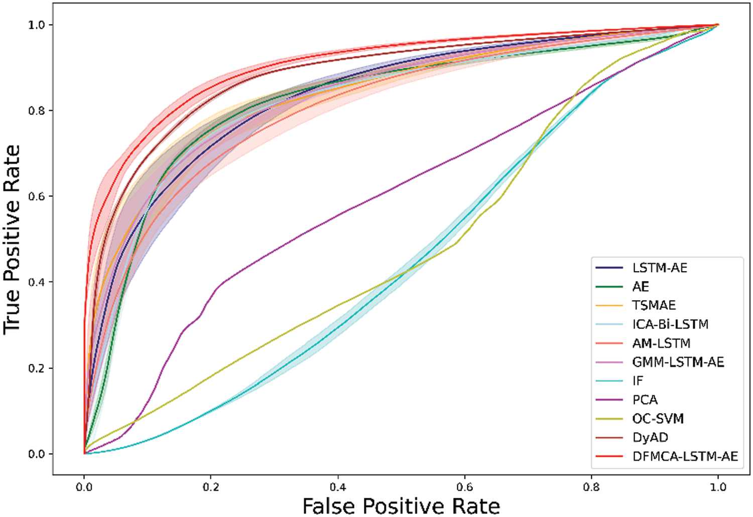
Figure 5: The average ROC curves for the eleven algorithms

The reconstruction of normal and abnormal samples by DFMCA-LSTM-AE on the LiB dataset is shown in Fig. 6. The blue curve represents the observed original samples, and the red curve indicates the reconstructed samples. ‘∆’ denotes normal samples, while ‘•’ signifies abnormal state samples. The pink area between the two curves represents the error. It can be seen that DFMCA-LSTM-AE reconstructs the normal samples well, with almost no discernible error compared to the observed values. In contrast, the reconstruction of the abnormal states samples is significantly different from the observed values, resulting in a conspicuous reconstruction error, which allows for a good distinction from the normal samples.

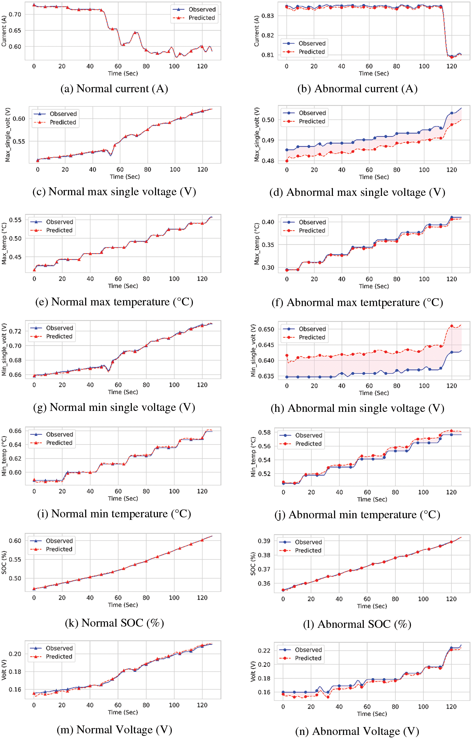
Figure 6: Comparison of reconstructed normal and abnormal samples

In summary, DFMCA-LSTM-AE significantly improves the detection of abnormal states in LiB time series by dynamically seizing frequency correlation and chronological relationships.

4.2.2 Ablation Experiments

To elucidate the function of each component within DFMCA-LSTM-AE, this section will showcase the ablation results for the modules. ‘DFMCA-LSTM-AE without DFMCA’ indicates that the model is stripped of the Dynamic Frequency Memory and Correlation Attention (DFMCA), with only the LSTM and linear layers remaining in both the encoder and decoder. ‘DFMCA-LSTM-AE without LSTM’ indicates the removal of LSTM layers from both the encoder and decoder, preserving just the DFMCA mechanism and linear layers. ‘DFMCA-LSTM-AE without Dyconv branch’ refers to eliminating the S2 and S3 pathways from the Dynamic Memory Fourier Transform module (DFTM, shown in Fig. 4), leaving only the pathway S1 intact. ‘DFMCA-LSTM-AE without Memory’ signifies not employing the Memory module within the DFTM. ‘DFMCA-LSTM-AE without hard threshold’ means that the Memory module does not implement a hard threshold to restrict the address vector.

The ablation results, as shown in Table 2, reveal that removing the DFMCA causes the model to fail to capture sufficient frequency correlation features, resulting in a significant drop in accuracy. Eliminating the LSTM layers leads to the inability to capture the relationships in the time series, which also decreases accuracy. Removing the dynamic convolution branches results in a decreased feature receptive field of the model, leading to a slight reduction in accuracy. Without the memory module, the model more effectively reconstructs abnormal samples’ frequency features and the samples themselves. Not implementing a hard threshold in the memory module causes too many minor memory items to combine, affecting the restoration of abnormal frequency features.

4.2.3 Memory Size

The dimension of the memory module N, essentially captures N representative normal frequency patterns, and by combining these patterns in varying proportions, it constructs a normal reconstructed sample as similar as possible to the original sample. The memory module can suppress the abnormal samples because the normal frequency features have a small set of unique characteristics in comparison to the abnormal frequency features, and the rest of the non-unique features are filtered out by the parameter adjustments during backpropagation and the operations of the hard threshold. This causes the model to only use that small part of features unique to normal frequency features during reconstruction, leading to poor reconstruction of abnormal frequencies. Therefore, it is important to reduce the dimensions of the memory module as much as possible without affecting the fit of the normal samples. Choosing an appropriate memory size thus becomes particularly crucial. Fig. 7 shows the impact of different memory sizes on the experimental results under the first fold of five-fold cross-validation. From the results in the figure, the model achieves the highest AUC and F1 when the memory size is 10, whereas there is a notable decline in performance when the memory size is 5, due to the inability to fit normal samples well at that point.

Figure 7: Performance of DFMCA-LSTM-AE with different memory sizes

4.2.4 Convolution Kernel Size and Step Size

Fig. 4 demonstrates the configuration of dynamic convolutions in two branches, S2 and S3. In branch S2, the convolution kernel’s size and stride, set to C, manage the medium-scale frequency features. Meanwhile, in branch S3, the kernel’s size and stride are larger, set to C2, allowing control over the large-scale frequency characteristics. Excessively large convolution kernels and strides will lead to serious impairment of frequency resolution, causing many important frequency characteristics to be missed, and failing to distinguish between normal and abnormal state frequencies. Fig. 8 demonstrates the impact of different C values on the experimental results under the first fold of five-fold cross-validation. It is evident that for the LiB dataset with a time length of 128, C values of 2 is the most suitable, as they increase the scale while retaining the fundamental information.

Figure 8: Performance of DFMCA-LSTM-AE with different C values

4.3 Model Interpretability Analysis

In this study, we specifically focus on the DFTM module in DFMCA-LSTM-AE, as it plays a crucial role in dynamically capturing multi-scale frequency relevancy and suppressing abnormal states. As shown in Fig. 9, the memory modules on the three branches of the Dynamic Memory Fourier Transform module (Fig. 4) were visualized. Fig. 9a corresponds to the memory module without dynamic convolution. Figs. 9b and 9c correspond to memory modules with dynamic convolution. It is apparent that the attention weights of the memory module without dynamic convolution are distributed relatively evenly throughout the entire chart. However, as the value of C increases, the distribution of attention becomes more extreme, especially in Fig. 9c, where the 1st, 3rd, and 4th rows have multiple consecutive dark cells, and the remaining rows have multiple consecutive light cells.

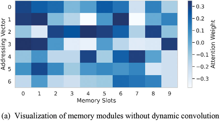
Figure 9: Visualization of the memory modules

This is because the features without dynamic convolution contain richer frequency information, requiring the memory module to maintain a more uniform distribution of attention to capture and utilize this information. When dynamic convolution is introduced as a filter, the model adjusts and reshapes the input features through a series of optimized filters. These filters act as learned weight matrices, selectively amplifying or attenuating different frequency components of the input data. It is similar to the way human vision searches for key information in complex scenes.

Furthermore, we conducted an interpretability analysis of the model’s inputs and outputs. As shown in Fig. 10, after the test set data was visualized using t-distributed stochastic neighbor embedding (T-SNE) and reduced to two dimensions, the abnormal samples were marked with red dots and the normal samples with grey dots. Fig. 10a shows the T-SNE result of the input data, where the red and grey dots are randomly mixed, with no discernible distance between clusters. Fig. 10b shows the T-SNE result of the output data from DFMCA-LSTM-AE, which reveals a clear inter-cluster distance between red and grey dots, indicating distinct clustering behavior. This clustering effect suggests that DFMCA-LSTM-AE has successfully learned the features necessary to differentiate between normal and abnormal patterns, demonstrating an understanding of the intrinsic structure of the data. Moreover, this clear spatial separation also suggests that the model has a good ability to distinguish unseen data, thereby proving its superior performance in abnormal state detection.

Figure 10: Input layer and the output layer of the DFMCA-LSTM-AE model with t-distributed stochastic neighbor embedding visualization

5  Conclusion

This paper addresses the challenge of accurately detecting abnormal states in lithium-ion battery (LiB) data, which is characterized by dynamic irregularities. Our important findings indicate that the DFMCA-LSTM-AE we proposed model not only overcomes the limitations of traditional methods but also demonstrates superior performance in detecting these abnormalities. Through the novel integration of a Dynamic Frequency Memory and Correlation Attention mechanism, our model dynamically recognizes frequency correlations and effectively suppresses the frequencies associated with abnormal samples. The incorporation of Long Short-Term Memory (LSTM) networks into the encoder and decoder components efficiently extracts temporal patterns within the time series data, further enhancing detection accuracy.

In extensive tests conducted on a dataset for abnormal state detection in lithium-ion batteries, DFMCA-LSTM-AE achieved impressive results. It recorded an average Area Under the Curve (AUC) of 90.73% and an average F1 score of 83.83%. These metrics indicate a substantial improvement over other models, with an increase in AUC ranging from 2.4% to 45.3% and an enhancement in F1 score from 1.6% to 28.9%.

Our study still has certain limitations, including the need for further validation of the model across various battery types and operational environments to ensure robustness and real-time performance. Our future work will focus on addressing these limitations. Training it with a small variety of LiB data to achieve good accuracy on a large variety of LiB data. Additionally, we plan to explore the use of shorter LiB time series to detect abnormal states, aiming to improve the model’s real-time performance.

Acknowledgement: The authors would like to thank the editor and anonymous reviewers for their valuable suggestions and comments.

Funding Statement: This research was partly supported by “Regional Innovation Strategy (RIS)” through the National Research Foundation of Korea (NRF) funded by the Ministry of Education (MOE) (2021RIS-002) and the Technology Development Program (RS-2023-00278623) funded by the Ministry of SMEs and Startups (MSS, Korea).

Author Contributions: The authors confirm contribution to the paper as follows: study conception and design: Haoyi Zhong, Chang Gyoon Lim; data collection: Yongjiang Zhao; analysis and interpretation of results: Haoyi Zhong, Yongjiang Zhao; draft manuscript preparation: Haoyi Zhong, Chang Gyoon Lim. All authors reviewed the results and approved the final version of the manuscript.

Availability of Data and Materials: The datasets are available at the links below: https://1drv.ms/u/s!AiSrJIRVqlQAgcjKGKV0fZmw5ifDd8Y?e=CnzELH237.

Conflicts of Interest: The authors declare that they have no conflicts of interest to report regarding the present study.

References

1. Inci, M., Savrun, M. M., Çelik, Ö. (2022). Integrating electric vehicles as virtual power plants: A comprehensive review on vehicle-to-grid (V2G) concepts, interface topologies, marketing and future prospects. Journal of Energy Storage, 55(2), 105579. [Google Scholar]

2. Ahmad, F., Alam, M. S., Alsaidan, I. S., Shariff, S. M. (2020). Battery swapping station for electric vehicles: Opportunities and challenges. IET Smart Grid, 3(3), 280–286. https://doi.org/10.1049/stg2.v3.3 [Google Scholar] [CrossRef]

3. Ciez, R. E., Whitacre, J. (2017). Comparison between cylindrical and prismatic lithium-ion cell costs using a process based cost model. Journal of Power Sources, 340(2017), 273–281. [Google Scholar]

4. Liu, K., Hu, X., Zhou, H., Tong, L., Widanage, W. D. et al. (2021). Feature analyses and modeling of lithium-ion battery manufacturing based on random forest classification. IEEE/ASME Transactions on Mechatronics, 26(6), 2944–2955. https://doi.org/10.1109/TMECH.2020.3049046 [Google Scholar] [CrossRef]

5. Pany, C., Tripathy, U. K., Misra, L. (2001). Application of artificial neural network and autoregressive model in stream flow forecasting. Journal of Indian Water Works Association, 33(1), 61–68. [Google Scholar]

6. Xiong, R., Li, L., Tian, J. (2018). Towards a smarter battery management system: A critical review on battery state of health monitoring methods. Journal of Power Sources, 405, 18–29. https://doi.org/10.1016/j.jpowsour.2018.10.019 [Google Scholar] [CrossRef]

7. Wang, F., Li, M., Mei, Y., Li, W. (2020). Time series data mining: A case study with big data analytics approach. IEEE Access, 8, 14322–14328. https://doi.org/10.1109/Access.6287639 [Google Scholar] [CrossRef]

8. Vamsi, A., ANSARİ, J., Krishnamoorthy, S. M., Pany, C., John, B. et al. (2021). Structural design and testing of pouch cells. Journal of Energy Systems, 5(2), 80–89. https://doi.org/10.30521/jes.815160 [Google Scholar] [CrossRef]

9. Tran, M., Fowler, M. (2020). A review of lithium-ion battery fault diagnostic algorithms: Current progress and future challenges. Algorithms, 13(3), 62. https://doi.org/10.3390/a13030062 [Google Scholar] [CrossRef]

10. Saxena, S., Kang, M., Xing, Y., Pecht, M. (2018). Anomaly detection during lithium-ion battery qualification testing. IEEE International Conference on Prognostics and Health Management (ICPHM), pp. 1–6. Seattle, WA, USA. [Google Scholar]

11. Liu, F. T., Ting, K. M., Zhou, Z. H. (2008). Isolation forest. Eighth IEEE International Conference on Data Mining, pp. 413–422. Pisa, Italy. [Google Scholar]

12. Hoang, D. H., Nguyen, H. D. (2018). A PCA-based method for IoT network traffic anomaly detection. 20th International Conference on Advanced Communication Technology (ICACT), pp. 381–386. Chuncheon, Korea (South). [Google Scholar]

13. Zhang, X., Liu, P., Lin, N., Zhang, Z., Wang, Z. (2023). A novel battery abnormality detection method using interpretable Autoencoder. Applied Energy, 330(2), 120312. [Google Scholar]

14. Jeng, S. L., Chieng, W. H. (2023). Evaluation of cell inconsistency in lithium-ion battery pack using the autoencoder network model. IEEE Transactions on Industrial Informatics, 19(5), 6337–6348. https://doi.org/10.1109/TII.2022.3188361 [Google Scholar] [CrossRef]

15. Thill, M., Konen, W., Wang, H., Bäck, T. (2021). Temporal convolutional autoencoder for unsupervised anomaly detection in time series. Applied Soft Computing, 112, 107751. https://doi.org/10.1016/j.asoc.2021.107751 [Google Scholar] [CrossRef]

16. You, G., Park, S., Oh, D. (2016). Real-time state-of-health estimation for electric vehicle batteries: A data-driven approach. Applied Energy, 176, 92–103. https://doi.org/10.1016/j.apenergy.2016.05.051 [Google Scholar] [CrossRef]

17. Ecker, M., Gerschler, J. B., Vogel, J., Käbitz, S., Hust, F. et al. (2012). Development of a lifetime prediction model for lithium-ion batteries based on extended accelerated aging test data. Journal of Power Sources, 215, 248–257. https://doi.org/10.1016/j.jpowsour.2012.05.012 [Google Scholar] [CrossRef]

18. Spigler, G. (2020). Denoising autoencoders for overgeneralization in neural networks. IEEE Transactions on Pattern Analysis and Machine Intelligence, 42(4), 998–1004. https://doi.org/10.1109/TPAMI.34 [Google Scholar] [CrossRef]

19. Hochreiter, S., Schmidhuber, J. (1997). Long short-term memory. Neural Computation, 9(8), 1735–1780. https://doi.org/10.1162/neco.1997.9.8.1735 [Google Scholar] [PubMed] [CrossRef]

20. Chen, Y., Dai, X., Liu, M., Chen, D., Yuan, L. et al. (2020). Dynamic convolution: Attention over convolution kernels. 2020 IEEE/CVF Conference on Computer Vision and Pattern Recognition (CVPR), pp. 11030–11039. Seattle, WA, USA. [Google Scholar]

21. Wang, Z., Hong, J., Liu, P., Liu, P., Zhang, L. (2017). Voltage fault diagnosis and prognosis of battery systems based on entropy and Z-score for electric vehicles. Applied Energy, 196(2017), 289–302. [Google Scholar]

22. Box, G. P., Pierce, D. A. (1970). Distribution of residual autocorrelations in autoregressive-integrated moving average time series models. Journal of the American Statistical Association, 65(332), 1509–1526. https://doi.org/10.1080/01621459.1970.10481180 [Google Scholar] [CrossRef]

23. Phillips, P. B., Jin, S. (2015). Business cycles, trend elimination, and the HP filter. Research Papers in Economics, 62(2), 469–520. [Google Scholar]

24. Kant, N., Mahajan, M. (2019). Time-series outlier detection using enhanced K-means in combination with PSO algorithm. Engineering Vibration, Communication and Information Processing, pp. 363–373. Jaipur, India, Springer Singapore. [Google Scholar]

25. Matias, P., Folgado, D., Gamboa, H., Carreiro, A. (2021). Robust anomaly detection in time series through variational autoencoders and a local similarity score. Proceedings of the 14th International Joint Conference on Biomedical Engineering Systems and Technologies, pp. 91–102. Vienna, Austria, Online Streaming. [Google Scholar]

26. Du, B., Sun, X., Ye, J., Cheng, K., Wang, J. et al. (2021). GAN-based anomaly detection for multivariate time series using polluted training set. IEEE Transactions on Knowledge and Data Engineering, 35(12), 12208–12219. [Google Scholar]

27. Wu, D., Jiang, Z., Xie, X., Wei, X., Yu, W. et al. (2020). LSTM learning with bayesian and gaussian processing for anomaly detection in industrial IoT. IEEE Transactions on Industrial Informatics, 16(8), 5244–5253. https://doi.org/10.1109/TII.9424 [Google Scholar] [CrossRef]

28. Meng, H., Zhang, Y., Li, Y., Zhao, H. (2020). Spacecraft anomaly detection via transformer reconstruction error. Proceedings of the International Conference on Aerospace System Science and Engineering 2019, pp. 351–362. Toronto, Canada. [Google Scholar]

29. Zhang, C., Song, D., Chen, Y., Feng, X., Lumezanu, C. et al. (2019). A deep neural network for unsupervised anomaly detection and diagnosis in multivariate time series data. Proceedings of the AAAI Conference on Artificial Intelligence, pp. 1409–1416. Hawaii, USA. [Google Scholar]

30. Zhang, J., Wang, Y., Jiang, B., He, H., Huang, S. et al. (2023). Realistic fault detection of Li-ion battery via dynamical deep learning. Nature Communications, 14(1), 5940. https://doi.org/10.1038/s41467-023-41226-5 [Google Scholar] [PubMed] [CrossRef]

31. Weston, J., Chopra, S., Bordes, A. (2015). Memory networks. International Conference on Learning Representations (ICLR), pp. 1130–1150. San Diego, CA, USA. [Google Scholar]

32. Sukhbaatar, S., Szlam, A., Weston, J., Fergus, R. (2015). End-to-end memory networks. Neural Information Processing Systems, vol. 28. [Google Scholar]

33. Kumar, A., Irsoy, O., Ondruska, P., Lyyer, M., Bradbury, J. et al. (2016). Ask me anything: Dynamic memory networks for natural language processing. International Conference on Machine Learning. PMLR, pp. 1378–1387. New York, NY, USA. [Google Scholar]

34. Chang, Y. Y., Sun, F. Y., Wu, Y. H., Lin, S. (2018). A memory-network based solution for multivariate time-series forecasting. arXiv:1809.02105. [Google Scholar]

35. Gao, H., Qiu, B., Barroso, R. J. D., Hussain, W., Xu, Y. et al. (2022). TSMAE: A novel anomaly detection approach for internet of things time series data using memory-augmented autoencoder. IEEE Transactions on Network Science and Engineering, 10(5), 2978–2990. [Google Scholar]

36. Hu, J., Shen, L., Sun, G. (2018). Squeeze-and-excitation networks. 2018 IEEE/CVF Conference on Computer Vision and Pattern Recognition, pp. 7132–7141. Salt Lake City, UT, USA. [Google Scholar]

37. Wang, Q., Wu, B., Zhu, P., Li, P., Zuo, W. et al. (2020). ECA-Net: Efficient channel attention for deep convolutional neural networks. Proceedings of the IEEE/CVF Conference on Computer Vision and Pattern Recognition, pp. 11534–11542. Seattle, WA, USA. [Google Scholar]

38. Gong, D., Liu, L., Le, V., Saha, B., Mansour, M. et al. (2019). Memorizing normality to detect anomaly: Memory-augmented deep autoencoder for unsupervised anomaly detection. Proceedings of the IEEE/CVF International Conference on Computer Vision, pp. 1705–1714. Seoul, Korea (South). [Google Scholar]

39. Paszke, A., Gross, S., Massa, F., Lerer, L., Bradbury, J. et al. (2019). PyTorch: An imperative style, high-performance deep learning library. Advances in Neural Information Processing Systems, vol. 32. Vancouver, Canada. [Google Scholar]

40. Kingma, D. P., Ba, J. (2014). Adam: A method for stochastic optimization. arXiv:1412.6980. [Google Scholar]

41. Zhang, X., Sun, J., Shang, Y., Ren, S., Liu, Y. et al. (2022). A novel state-of-health prediction method based on long short-term memory network with attention mechanism for lithium-ion battery. Frontiers in Energy Research, 10(2022), 972486. [Google Scholar]

42. Sun, H., Sun, J., Zhao, K., Wang, L., Wang, K. (2022). Data-driven ICA-Bi-LSTM-combined lithium battery SOH estimation. Mathematical Problems in Engineering, 2022, 1–8. [Google Scholar]

43. Malhotra, P., Ramakrishnan, A., Anand, G., Vig, L., Agarwal, P. et al. (2016). LSTM-based encoder-decoder for multi-sensor anomaly detection. arXiv:1607.00148. [Google Scholar]

44. Lee, J. G., Kim, D. H., Lee, J. H. (2023). Proactive fault diagnosis of a radiator: A combination of gaussian mixture model and LSTM autoencoder. Sensors, 23(21), 8688. https://doi.org/10.3390/s23218688 [Google Scholar] [PubMed] [CrossRef]