Traffic Flow Prediction with Heterogeneous Spatiotemporal Data Based on a Hybrid Deep Learning Model Using Attention-Mechanism

1  Introduction

The performance of traffic flow prediction is the foundation for dynamic strategies and applications in intelligent transportation systems. This issue holds immense practical importance for enhancing traffic safety and alleviating road congestion. This predicting capability enables effective decision-making for traffic management, encompassing adjustments to traffic signals and the implementation of temporary traffic control measures. Hence, it has progressively garnered the interest of numerous researchers [1–4], with extensive usage in detecting transportation anomalies [5,6], optimizing resource allocation [7], managing logistics supply chains [8], and overseeing urban administration [9,10].

Traffic flow typically has inherent patterns, suggesting it is generally possible to predict it accurately. Over the past few decades, significant research has been conducted on predicting traffic flow. Various methods have been explored, including the autoregressive integrated moving average (ARIMA) approach [11], support vector regression (SVR), and K-nearest neighbors (KNN) [12]. ARIMA is a parametric model that relies on rigorous theoretical assumptions [13,14]. It works in a basic linear model. Most conventional parameter models are characterized by simplicity and efficiency in computation. However, they exhibit limited robustness and are better suited for road sections with consistent traffic circumstances. Consequently, it cannot reliably predict traffic flow, which is complex and nonlinear [15,16]. As a result of the previously described shortcomings of conventional statistical models, researchers gravitated towards machine learning models.

Machine learning models such as SVR and KNN provide adaptability as they can acquire knowledge from the data. Nevertheless, the prediction performance of these techniques remains unsatisfactory as they solely account for the temporal fluctuations of traffic flow, disregarding its stochastic and nonlinear characteristics. Moreover, the conventional machine learning approaches rely on manually designed parameters to seize the properties of traffic flow. Another limitation of classical machine learning is the laborious task of manually extracting features [15]. This condition creates a high dependency on domain experts in certain fields and causes insufficient for achieving precise prediction performance.

Presently, two distinct perspectives exist on enhancing performance in deep learning (DL), specifically the model-centric and the data-centric approaches. In a model-centric context, the researcher iteratively enhances the designed model (algorithm/code) while keeping the quantity and kind of acquired data constant. On the other hand, researchers of the data-centric approach adhere to static models while consistently enhancing the quality of the data [17]. Deep learning has made significant advancements in recent years, demonstrating exceptional achievements in diverse fields such as speech recognition and computer vision. In contrast to conventional artificial neural network (ANN) models, deep learning models employ multi-layer structures to retrieve intrinsic features from extensive raw data sets automatically. Due to the influence of deep learning, there has been a notable increase in enthusiasm for transportation research in recent years. Numerous deep-learning techniques for predicting traffic flow have been proposed [18–21]. In recent times, there has been a notable improvement in the predictive performance of deep models, including the variance of long short-term memory network (LSTM) [22] and convolutional neural network (CNN) [23], which can be attributed to their robust ability to effectively capture temporal or spatial dependencies, surpassing the performance of shallower models.

Nonetheless, current studies that rely on neural network models for traffic flow prediction encounter the following limitations. Certain studies utilize basic neural network models like stacked autoencoders (SAE), LSTM, or CNN, failing to capture traffic flow’s intricate characteristics adequately; as a result, these models offer only marginal improvements in prediction performance. Typically, LSTM captures temporal characteristics, while CNN extracts spatial features. LSTMs are inherently unidirectional, which implies that they can handle information sequentially, moving from the past to the future. This condition can provide a constraint when dealing with worldwide scope and interdependencies in both directions. Addressing this issue, bidirectional long short-term memory (BiLSTM) was designed to process information from the past and future simultaneously, enabling the model to gain a more comprehensive knowledge of the whole context of the data series [24]. CNN excels at obtaining highly effective spatial information. However, it has difficulties when it comes to extracting temporal aspects. The two models mentioned above are often utilized independently for each distinct situation. By combining the advantages of both models, it is possible to overcome existing challenges associated with the complex and nonlinear spatiotemporal properties of traffic flow data.

Moreover, existing studies do not fully exploit the complex structure present in traffic flow data. They solely employ attention methods on a single network layer, neglecting to allocate attention to the remaining layers [25]. Several variables impact the performance of traffic flow prediction. They disregard the significance of conditions or occurrences at a specific location or during specific time intervals in previous traffic patterns, which are crucial in making precise predictions about future traffic patterns [26,27]. Here, we propose a unique hybrid deep learning Conv-BiLSTM method incorporating an attention mechanism to tackle the abovementioned issues. This methodology utilizes heterogeneous multi-periodic intra-spatiotemporal data to improve the performance of traffic flow prediction. The main contributions of this paper are as follows:

•   In this study, we proposed a novel hybrid deep learning model incorporating Conv-BiLSTM networks and BiLSTM using an attention mechanism to leverage traffic flow’s spatiotemporal and periodicity characteristics effectively. In contrast to the current hybrid model utilized for traffic flow prediction, the Conv-BiLSTM model demonstrates enhanced efficiency in capturing spatiotemporal data. The efficiency is achieved by processing spatial and temporal features together, improving predictive performance.

•   Attention mechanisms are developed for Conv-BiLSTM and BiLSTM modules to dynamically assign varying levels of attention to a sequence of traffic flows at distinct temporal instances. The suggested system can autonomously differentiate the significance of each flow sequence’s contribution to the ultimate prediction performance outcome.

•   This study combines two methodologies: the model-centric approach and the data-centric approach. In the context of the data-centric approach, we include intra-data to segregate traffic flow into distinct categories depending on five vehicle types rather than aggregating them into a single count of vehicles.

•   In this study, our approach collects heterogeneous spatiotemporal data features (holidays, weather, and vehicle type) at current, daily, weekly, and monthly periodicities that previous studies have not implemented to improve prediction performance.

The subsequent sections of this work are structured in the following manner. In Section 2, the data representation is introduced. Section 3 introduces a unique deep-learning methodology for predicting traffic flow. In Section 4, we undertake tests on the dataset and evaluate the predictive performance compared to many current approaches. Section 5 presents the conclusion and future research.

2  Research Data

The traffic flow dataset used in this study was obtained from the Taiwan Ministry of Transportation, which can be accessed publicly in the Traffic Data Collection System (TDCS) (https://tisvcloud.freeway.gov.tw/history/TDCS/M06A/). The dataset presented in this research encompasses pertinent information on the number of cars observed on the Taiwan National Freeway. This study focused on observing the traffic flow at eight gantries along Taiwan National Freeway No. 3 from November 2016 to October 2019 (3 years). The input of this paper is from the output of frequency distributions of repeats extracted from vehicle trips via previous approaches developed in [28,29]. On the other hand, there was another similar work to have maximal repeat extraction from bus passenger’s trips [30]. Apart from data on the traffic flow, this research also involves other features such as weather (https://openweathermap.org/) and holiday (https://timeanddate.com) data. Detailed feature information can be found in Table 1.

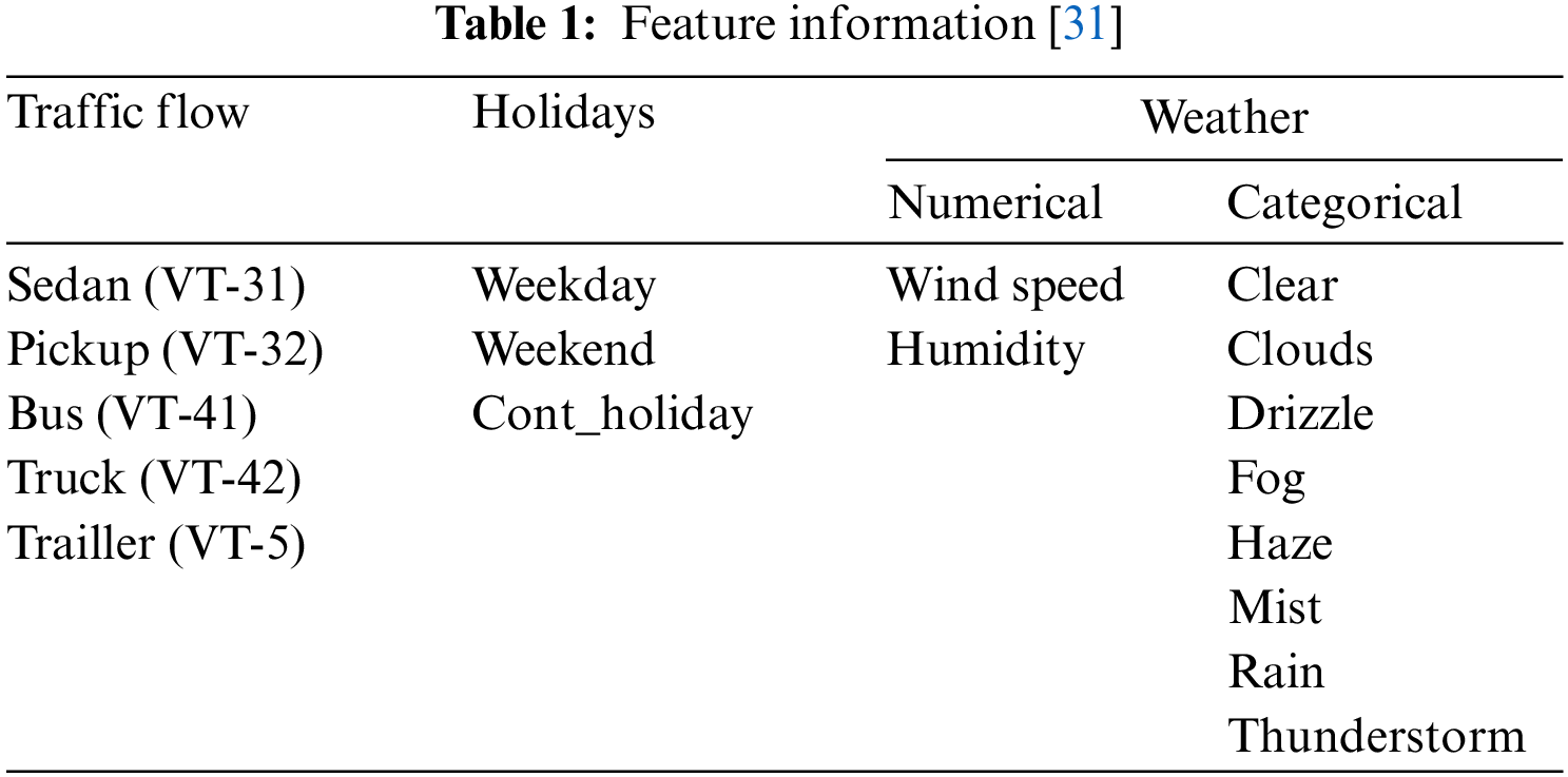
The weather feature is classified into two distinct categories: numerical and categorical. The wind speed measurements consist of decimal values spanning from 0 to 15.95, while the humidity readings are whole numbers ranging between 0 and 100. Conversely, various weather conditions are distinguished by boolean values. Holidays fall into three categories: weekday, weekend, and cont_holiday. The weekday category pertains to holidays occurring on any day from Monday to Friday. The weekend condition refers to holidays that occur on Saturdays or Sundays. The cont_holiday condition encompasses holidays that may occur either prior to or following weekdays or weekends. Meanwhile, for vehicle types, we divide traffic flow into five categories (sedan, pickup, bus, truck, trailer). Detailed data preprocessing can be seen in the previous research [31].

Successful traffic flow prediction models must accurately capture the random and nonlinear characteristics of transportation traffic conditions. Numerous traffic models based on statistics or machine learning techniques have been developed to enhance the accuracy of predictions. One of the crucial processes of machine learning is feature learning. The process entails extracting and selecting the most significant aspects from past traffic flow data.

The characteristics of traffic flow commonly display spatiotemporal correlation and periodic patterns. Specifically, the traffic flow at the observation area is influenced by the traffic conditions of nearby locations and affected by previous time intervals. Traffic flow also demonstrates periodic patterns on a current, daily, weekly, and monthly basis. For example, the traffic flow variation on the same day for two consecutive weeks exhibits remarkable similarity. What is rarely considered is the monthly periodicity, even though monthly periodicity is the most pronounced pattern compared to daily and weekly periodicity. For instance, it can be related to weather or holiday patterns. Generally, weather conditions and holidays within a country tend to remain relatively consistent, unlike daily and weekly periodicity, which are more random. This research paper introduces a deep learning model that utilizes spatiotemporal correlation and periodic characteristics to enhance short-term traffic flow prediction.

Predicting traffic flow aims to enhance transportation efficiency by delivering precise and timely information regarding upcoming traffic conditions. The issue of predicting traffic flow can be stated in the following manner. Consider that XTp represents the traffic flow throughout the T th time interval. The observed feature can refer to vehicle types, weather, or type of holiday. The observed prediction target in this research is vehicle-type sedan (VT-31) traffic flow. Given the historical traffic flow sequence of observed feature, the objective at the current time t is to forecast the traffic flow at the time interval (t + h Δ), where Δ represents the prediction horizon {XTp}(T) = t – nΔ, …, t – Δ, t, and p ∈ P, where P is the set of observation features. This study considers the following parameters: Δ = 1 h, n = 12, and h = 1. n indicates that we utilize a historical dataset spanning 12 h to forecast the traffic flow for the upcoming one hour. For simplicity in explanation, we represent t – n as t – nΔ by excluding the Δ symbol in this paper.

Before presenting our traffic flow prediction model, we explain the process of creating a historical dataset for this research. Here, we represent time series numerical data from the dataset as an image, adopting the approach carried out in previous research [31]. Let ftp represent the value of each observation feature p at time t. Each feature in Table 1 undergoes a normalization step to ensure that its data value falls within the range of [0,1]. The representation of the historical observation feature p can be expressed as XTp = [f0p,…,fTp].

Next, we combine all features (p features) to generate a matrix representing the spatiotemporal traffic flow. Where Ç´tp = [ft1,ft2,…,ftp] designates the observation feature of the prediction-based current periodic (c) at time t.

Ç´tp=[ft−n1ft−(n+1)1…ft1…ft+n1ft−n2ft−(n+1)2…ft2…ft+n2⋮⋮⋮⋮⋱⋮ft−npft−(n+1),p…ftp…ft+np](1)

Furthermore, we contemplate the periodic characteristics of the traffic flow and other features. We consider daily (d), weekly (W¨), and monthly (m˙) patterns to create historical data and incorporate all features with periodicity. The traffic data that shows a daily pattern can be obtained by considering the n time intervals before and after the precise moment t on the previous day. This can be stated as:

Dtp=[ft−d−n1ft−d−n+11…ft−d1ft1…ft+n1ft−d−n2ft−d−n+12…ft−d2ft2…ft+n2⋮⋮⋮⋮⋮⋱⋮ft−d−npft−d−n+1p…ft−dpftp…ft+np](2)

where d designates the exact instant as time t on the last day. Likewise, we obtain historical traffic flow data that exhibits a weekly pattern by analyzing the time intervals before and after the same instant in the previous week, denoted as time t. We employ the following method:

W¨tp=[ft−w¨−n1ft−w¨−n+11…ft−w¨1ft1…ft+n1ft−w¨−n2ft−w¨−n+12…ft−w¨2ft2…ft+n2⋮⋮⋮⋮⋮⋱⋮ft−w¨−npft−w¨−n+1p…ft−w¨pftp…ft+np](3)

where W¨ indicates the identical point as time t in the last week, month patterns are denoted as combined data from the current month and the previous month.

M˙tp=[ft−m˙−n1ft−m˙−n+11…ft−m˙1ft1…ft+n1ft−m˙−n2ft−m˙−n+12…ft−m˙2ft2…ft+n2⋮⋮⋮⋮⋮⋱⋮ft−m˙−npft−m˙−n+1p…ft−m˙pftp…ft+np](4)

The visual depiction of the merging process for each data by period can be seen in Fig. 1. The dataset marked as “blue” encompasses historical data over the preceding 12-h period. In contrast, the dataset marked as “orange” pertains to historical data, specifically from the corresponding time of the current day. The “purple” data represents the 12-h historical records of the preceding week, whereas the “brown” segment encompasses the identical dataset from the preceding month. The combination of each data is represented as current, daily, weekly, and monthly periodic data, as mentioned below.

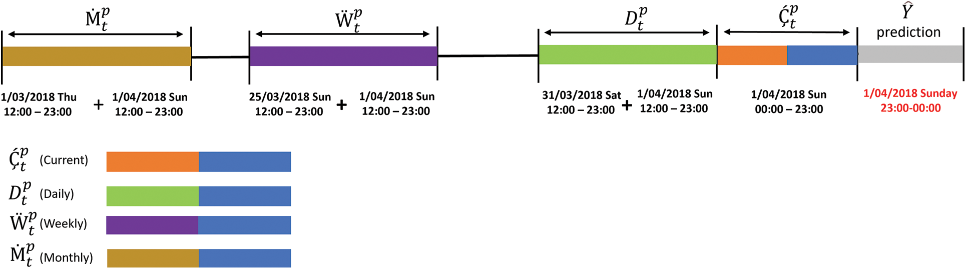
Figure 1: Data input representation

3  Proposed Method

This section explains the proposed hybrid model for predicting traffic flows. The proposed model consists of a Conv-BiLSTM module and three BiLSTM modules. This part of the proposed method can be seen in Fig. 2. In the first step, the primary objective of the convolutional network is to extract spatiotemporal information. The data set used in this research consists of heterogeneous data covering three aspects: traffic flow, holidays, and weather with different periodicity patterns. Convolutional models are most suitable for managing this type of data. In the second step, the primary purpose of BiLSTM is to extract information from the temporal characteristics of traffic flows. This model will extract crucial data based on periodic patterns for each feature. In prior studies, the authors [25] employed a comparable methodology. One notable distinction is how the input data is structured for the Conv-BiLSTM and BiLSTM layers.

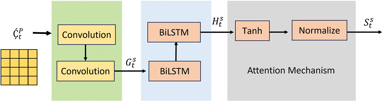
Figure 2: Conv-BiLSTM with attention mechanism

Previous studies have utilized homogenous inter-data traffic flow from two distinct geographical areas [25]. The data on homogeneous traffic flow does not provide distinctions among various types of vehicles. In this investigation, we employed heterogeneous intra-data [27], which refers to data collected from a specific area (eight gantries in Taiwan National Freeway No. 3). This research categorizes traffic flow data based on five different types of vehicles (sedan, pickup, bus, truck, trailer). Furthermore, we have incorporated an attention mechanism that operates in the Conv-BiLSTM layer and across all model layers. Running this strategy enables the model to dynamically assess the varying significance levels of flow sequences at different periodic instances. The subsequent subsections will provide a comprehensive explanation of each module.

3.1 Conv-BiLSTM

The Conv-BiLSTM module serves as the primary constituent of the model that has been suggested, seeking to derive spatiotemporal characteristics from the traffic flow. The Conv-BiLSTM module integrates a convolutional neural network with a Bidirectional Long Short-Term Memory (BiLSTM) network, as depicted in Fig. 2. The architecture in the first stage consists of two convolutional layers. In the next stage, it passes through two BiLSTM layers.

The Conv-BiLSTM model takes as input spatiotemporal data derived from three distinct features, which are denoted as the current periodic matrix Ç´tp. This matrix, as denoted in Eq. (1), represents the historical data that is to be forecasted. To acquire the spatiotemporal feature, a one-dimensional (1-D) convolution operation is conducted on the traffic flow data Ç´tp at each time step t. Pooling is not performed in the convolution layer. The output of the last convolution layer (layer 2) within this particular layer is represented as Gts. Furthermore, the output of the convolutional layer is subsequently utilized as the input for the BiLSTM layer. In this study, to improve the performance of traffic flow prediction, we leverage the BiLSTM models, which can capture temporal characteristics of traffic data by employing contextual information from two-directional. The bidirectional character of BiLSTM models enables them to capture long-term dependencies present in the data more efficiently. Individuals can retain and recall information from preceding and subsequent sequence segments. This cognitive function is important in activities necessitating comprehension of the whole context.

The initial BiLSTM layer is tasked with processing the sequential output derived from the final convolution layer, GTs=Gt−ns,…,Gt−1s,Gts, spanning from the beginning to the last. This section computes the hidden state value for each time step H1,Ts=H1,t−ns,…,H1,t−1s,H1,ts. Next, the concealed state sequence H1,Ts is fed into the second BiLSTM layer to compute the hidden state H2,Ts at time step t, which serves as the output of the complete BiLSTM network HTs. The output of this last BiLSTM layer subsequently serves as the input for the attention mechanism, which will be elaborated on in the following section.

3.2 Bi-Directional LSTM for Temporal Dependency

Acquiring temporal dependence is another crucial challenge in traffic flow prediction. Recurrent neural network (RNN) is frequently employed to process data that exhibits sequential properties. The Elman Network, introduced by Elman in 1990, is considered the most typical and fundamental version of the standard RNN frequently utilized [32]. Nevertheless, the conventional RNN often encounters gradient explosion and gradient disappearance issues while handling lengthy time series data. The LSTM cell incorporates three control gates: the input, forget, and output. These gates utilize three techniques to regulate the flow of information inside the network, enabling the implementation of long-term memory. Fig. 3 illustrates the conventional configuration of the LSTM cell.

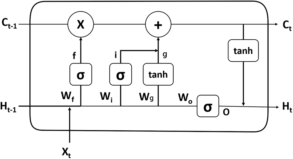
Figure 3: The LSTM network structure [31]

Fig. 3 depicts Xt as the parameter input value of the LSTM cell at a specific moment t, Ct as the state value of the memory cell and ht as the hidden value output at time t. Wf, Wi,Wg, Wo, and b represents the weights matrix and bias of each threshold layer. The term tanh refers to the tanh activation function, while σ denotes the sigmoid activation functions. The internal computation method of LSTM can be elucidated through Eqs. (5) to (10):

Step 1: Compute the activation value ft of the forget gate at time t using the following formula:

ft=σ(Wf[Xt;Ht−1]+bf)(5)

Step 2: The next step is to calculate the numerical value of the input gate it and the candidate’s state gt of the cell at time t. The precise calculating formulas are as follows:

it=σ(Wi[Xt;Ht−1]+bi)(6)

gt=tanh(Wg[Xt;Ht−1]+bg)(7)

Step 3: Compute the value Ct for updating the cell state at time t using the following formula:

Ct=ft×Ct−1+it×gt(8)

Step 4: Compute the value of the output variable ot of the output gate at time t using the following formula:

ot=σ(Wo[Xt;Ht−1]+bo)(9)

Ht=ottanh⁡(Ct)(10)

Fig. 4 depicts the bidirectional LSTM network, which includes forward and backward Long Short-Term Memory (LSTM) models. The forward LSTM processes information in one way, while the reverse LSTM processes information in the opposite direction. The input sequence undergoes processing by the forward LSTM layer, given the output HTforward(HTf), while the reverse form of the input sequence is inputted into the backward LSTM layer, given the output HTbackward(HTb).

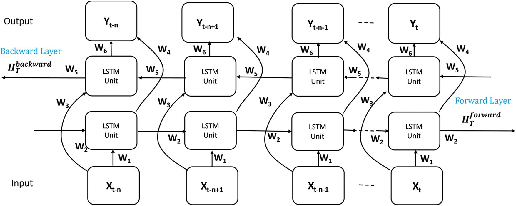
Figure 4: The structure of the BiLSTM network

Ultimately, the concealed states of the forward and backward layers are combined to form the output. The basic LSTM’s limitation of just utilizing prior information is resolved, and the prediction performance is enhanced by implementing two unidirectional LSTMs. We utilize the BiLSTM to capture the temporal correlation of traffic flow in our study. Fig. 5 depicts the general structure of the BiLSTM module utilized in the proposed model. In this module, Dtp, W¨tp, and M˙tp represent the input of the LSTM. Htd,f, Htw,f and Htm,f represent the output of the forward LSTM while Htd,b, Htw,b and Htm,b represent the backward LSTM output when the inputs are Dtp, W¨tp, and M˙tp, respectively. To account for the regularity of traffic data, we employ numerous BiLSTM layers to extract recurring characteristics from past traffic data.

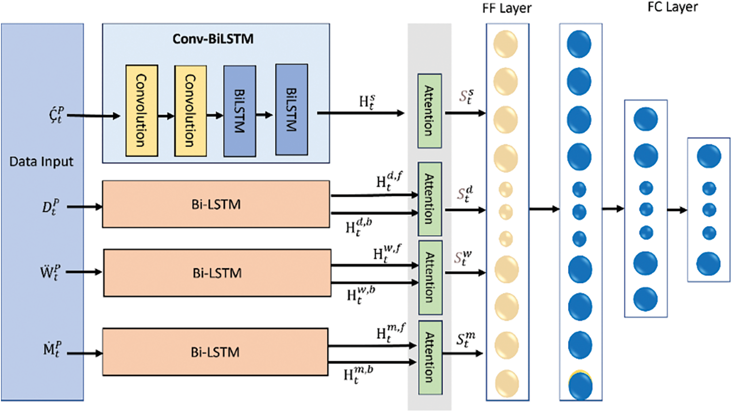
Figure 5: The proposed model

3.3 Attention Mechanism Based on Temporal Dependency

The attention mechanism approach has been extensively used across various domains, including natural language processing, image processing, and speech recognition. For example, the utilization of attention mechanisms to enhance translation accuracy initially emerged in the context of translation machines [1,33]. In short, the attention mechanism directs its emphasis on information that significantly influences the results and reduces the weight of unimportant information during the feature extraction process. The relative significance of traffic flow data at various time intervals may vary concerning the forecasting objective. In the domain of traffic flow prediction, a similar phenomenon is observed, where the influence of traffic flow varies at different periods, affecting the relevance of prediction performance [25]. The variability of traffic conditions at a given observation site can exhibit temporal fluctuations when forecasting traffic flow at the site of an observation area. In instances of congestion, the anticipated outcome may be more significantly impacted by the traffic conditions observed at a remote point instead of those observed at a closer point.

However, the conventional BiLSTM model cannot determine which segments of a traffic flow sequence are essential or significant. We have devised a dedicated attention mechanism tailored for the Conv-BiLSTM module to tackle this problem. This mechanism enables automatic identification and utilization of varying importance’s level within a traffic flow sequence at different time points. We divide the temporal dependency into four categories based on the characteristics of the traffic data: current, daily, weekly, and monthly period. The link between multiple recent time intervals and the desired one is referred to as the current pattern; for example, traffic conditions at 10:00 am will influence the situation at 11:00 am. The current, daily, weekly, and monthly patterns reference the recurring character of human behavior. For instance, weekday traffic patterns vary similarly, with distinct morning and evening rush hours. Additionally, the morning rush hour periods may be postponed due to later weekend wake-up times.

An attention method is employed to dynamically modify the weighting of the output from the BiLSTM module. The expression of the attention mechanism’s implementation can be formulated as follows:

µit=tanh⁡(Wωhit+bω)(11)

βit=exp(µitTµω)∑texp(µitTµω)(12)

Si=∑tβithit(13)

The learnable parameters in this context are denoted as Wω, bω, and μω. The attention score is represented by βit, and the output of the attention layer is denoted as Si.

3.4 Output Layer

Following the attention layer, the spatiotemporal and periodicity features derived from the three network components are consolidated into a feature vector via a feature fusion layer. Assuming that X ∈RN×C represents the input to the output layer, a two-layer fully connected neural network is employed to predict a single timestep. T two-layer fully connected neural networks are employed to predict T future timesteps. The final forecast is derived by aggregating the prediction results from each timestep. The specific process can be outlined as follows:

y^(i)=ReLU(XW1(i)+b1(i))×W2(i)+b2(i)∈RN×1(14)

Y^=[y^(1),y^(2),…y^(T)]∈RN×T(15)

where the variable y^(i) represents the timestep used for making predictions at time i, W1(i)∈RN×1,b1(i)∈RC ′,W2(i)∈RC ′×1, and b2(i)∈R represents the parameters that can be learned. The dimension of the output of the first fully linked layer is denoted as C ′. We use Y^ and y^ to designate the predicted and ground truth values. Table 2 shows a training algorithm for a Conv-BiLSTM model.

4  Experimental Result

4.1 Metaparameter Settings

The proposed model was constructed utilizing the TensorFlow framework, and the experiments were carried out on a Google Collaboration Pro Plus platform equipped with a T4 GPU. The experiment involved a model that consisted of two convolution processes with three filters and 256 hidden units of BiLSTM. Using our dataset as a case study, we varied the size of the kernel convolution layer from 2 to 11. We employed a two-layered BiLSTM architecture to capture the periodic patterns in the traffic data effectively. Assign the optimization technique used was Adam, with an initial learning rate of 0.001, a batch size of up to 128, and an epoch size of 500 for this model. This Adam optimization technique was chosen since it has the capability to modify the learning rate adaptively. We adopt the Conv-LSTM model as a benchmark model, following the specifications specified in the research [19]. To determine how to assess the efficacy of the suggested model, we employed the mean absolute error (MAE) metric [34]. These parameters include a filter of size 10, a kernel size of 3, and a batch size of 128. The evaluation results using this model produced an MAE value of 21.041.

4.2 Proposed Model Performance

We performed comparison experiments using the following short-term traffic flow prediction methodologies to assess the prediction performance of the proposed model: Conv-LSTM, CNN-LSTM, and CNN-BiLSTM. We employ two scenarios, with the first scenario including applying the attention mechanism solely to the first layer of Conv-BiLSTM. Furthermore, every layer employs an attention technique. Fig. 6 shows the best prediction model performance based on their feature and kernel size. The selection of kernel size is essential in determining the performance of convolutional neural networks. The kernel is a compact window that traverses the input data to extract distinctive characteristics. The choice of kernel size directly impacts the network’s capacity to capture spatial information in the input. Greater kernel sizes efficiently capture comprehensive patterns and advanced characteristics, although they can result in heightened computing intricacy and necessitate a larger number of parameters. Conversely, smaller kernel sizes excel in capturing intricate details and specific traits, improving parameter utilization. Ensuring the appropriate equilibrium of kernel sizes is crucial for attaining peak performance in a convolutional network, as it dictates the network’s ability to acquire hierarchical representations and effectively adapt to various inputs. Evaluating the kernel size and other architectural decisions is crucial for creating convolutional networks that perform exceptionally well in different computer vision tasks.

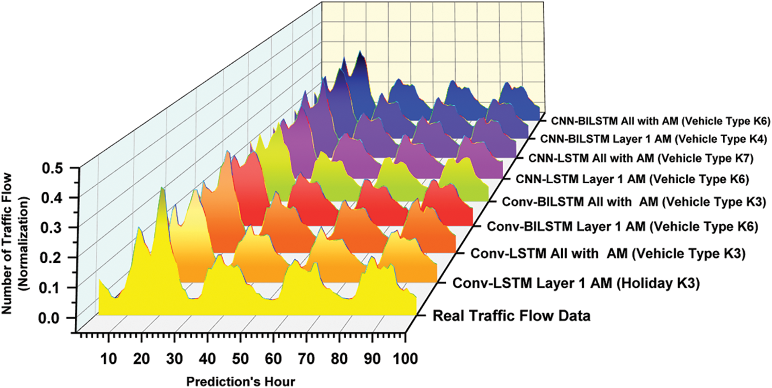
Figure 6: The best performance of all the prediction models with its features and kernel size

Fig. 7 indicates that the Conv-BiLSTM model, with vehicle type feature as input, generates the greatest performance among other models when employing a kernel size of 3 and applying an attention mechanism to each layer.

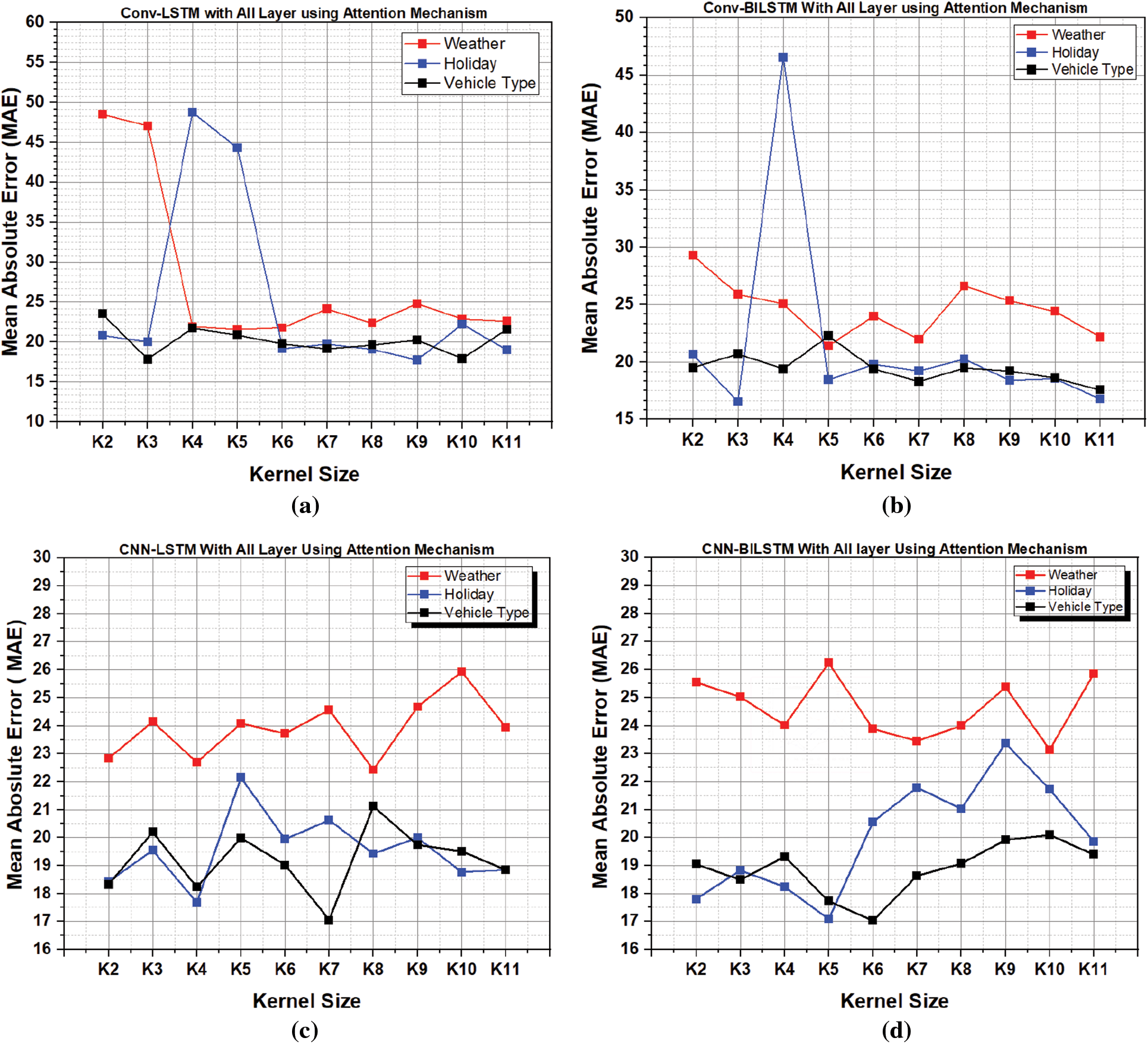
Figure 7: The effect of convolution kernel size on the traffic flow prediction model performance. (a) Conv-LSTM with all layer attention mechanism, (b) Conv-BiLSTM with all layer attention mechanism, (c) CNN-LSTM with all layer attention mechanism, (d) CNN-BiLSTM with all layer attention mechanism

Tables 3 and 4 display the performance of various methods in predicting traffic flow over the next hour. Based on the data presented in the table, it is evident that the proposed model (Conv-BiLSTM with all layers using attention mechanism) outperformed all other models regarding the evaluation metrics with a mean absolute error (MAE) value of 16.478. There was a performance increase of 21,68%. Across several prediction models, the vehicle type feature consistently exhibits the lowest loss value. These findings indicate that the vehicle type attribute has the greatest influence on the performance of the results for prediction.

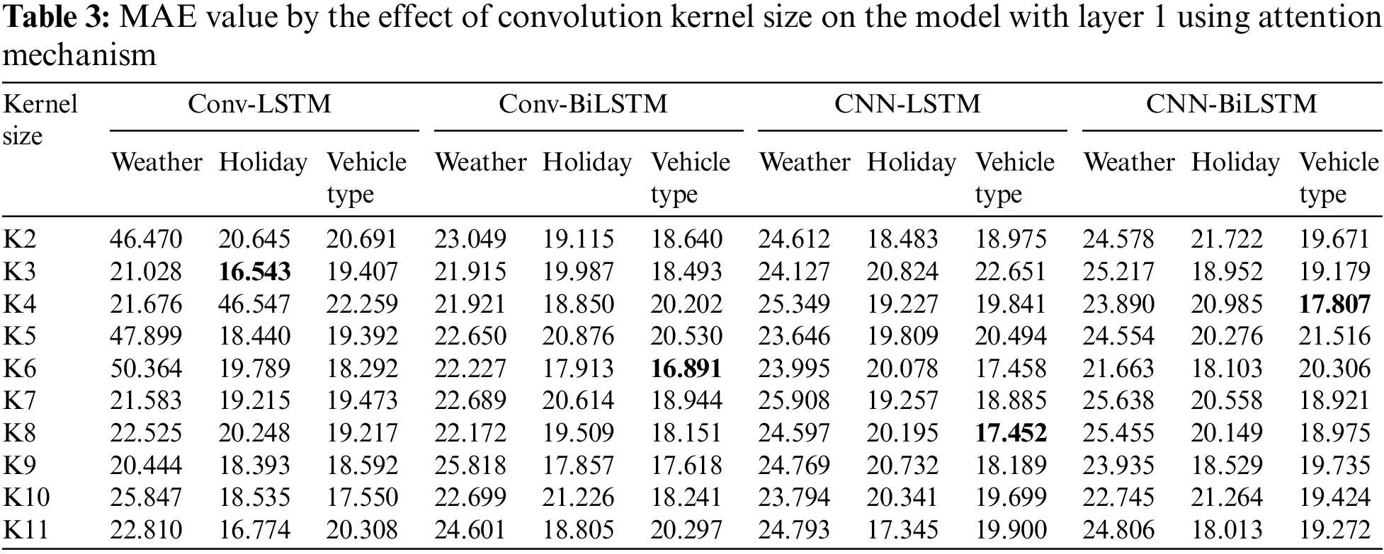
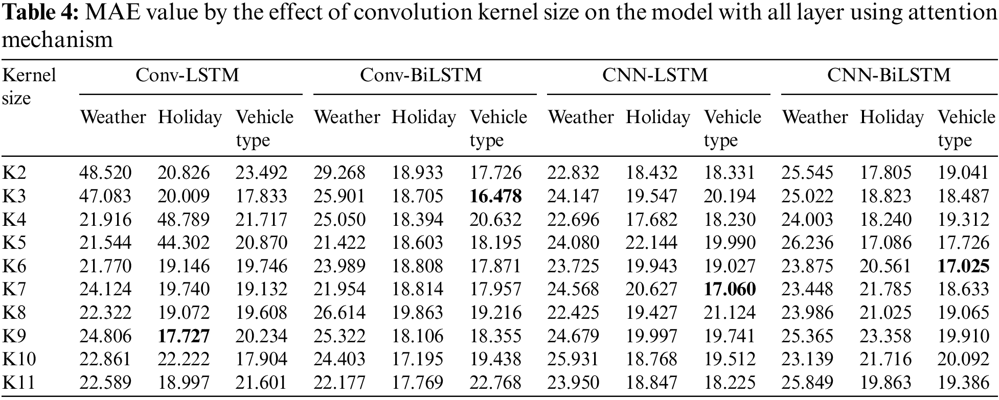
Fig. 8 illustrates the impact of features and kernel sizes on each model when all layers use an attention mechanism. Fig. 8a, by utilizing weather data as input, the Conv-LSTM model’s performance is subpar while employing kernel sizes of 2 and 3. Conv-LSTM’s performance improves when the kernel size exceeds 3, comparable to other models. The Conv-BiLSTM model achieves optimal performance with a kernel size of 5, as depicted in Fig. 8a. Fig. 8c demonstrates the input data related to the vehicle type of various periodicities significantly influences the model’s performance. Employing kernel sizes between 2 and 6 demonstrates a propensity for achieving favorable performance outcomes. Meanwhile, kernels with a value larger than 6 have negligible effect.

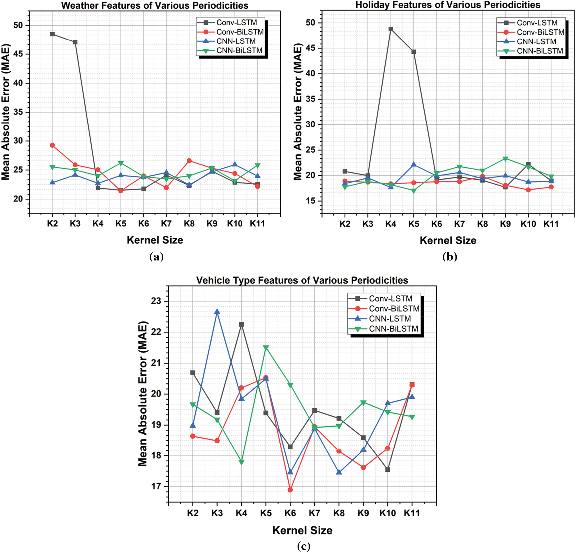
Figure 8: The effect of convolution kernel size on the traffic flow prediction model performance based on input data feature to proposed model using all layers with attention-mechanism. (a) Weather features of various periodicities, (b) holiday features of various periodicities, (c) vehicle type features of various periodicities

Based on the conducted studies, incorporating vehicle-type variables had the most significant effect on enhancing prediction performance, resulting in a 21.68% increase when utilizing the Conv-BiLSTM model. Table 4 demonstrates the fluctuation in error reduction when comparing various kernel sizes for each traffic flow prediction model using a model that incorporates attention techniques in all layers. The Conv-LSTM model has optimal performance when using a kernel size of 9 in combination with the holiday feature. Meanwhile, the Conv-BiLSTM model, which yields the most significant performance improvement when utilizing a kernel size of 3, incorporates the vehicle type feature. On the other hand, the CNN-LSTM and CNN-BiLSTM models, which have kernel sizes of 7 and 6, respectively, demonstrate the best performance when considering the vehicle type feature.

5  Conclusion and Future Research

This study examines the short-term traffic flow prediction by utilizing the dataset provided by the Taiwan Ministry of Transportation, specifically focusing on the number of cars on Taiwan National Freeway No. 3. The hybrid deep learning model that combines convolutional neural networks and BiLSTM networks was suggested as a way to deal with the complex and nonlinear features of traffic flow. The results of our study suggest that the Conv-BiLSTM model, which incorporates an attention mechanism, effectively captures spatiotemporal data. Furthermore, integrating the suggested attention mechanism throughout all layers amplifies the Conv-BiLSTM’s efficacy in enhancing prediction performance. The traffic flow prediction model effectively catches repeating trends on a current, daily, weekly, and monthly basis, hence improving the performance of predictions. Integrating diverse features such as holidays, weather conditions, and vehicle types has benefited prediction models. The Conv-BiLSTM model, when combined with the vehicle type feature, enhances prediction performance by 21.68%. Empirical evidence shows that this strategy surpasses earlier methodologies in traffic flow prediction.

Current research only emphasizes capturing spatiotemporal correlations based on the nature and dynamics of traffic flow features. However, it has not paid attention to the Euclidean nature of the road structure, such as paying attention to the linkage of traffic flow information between road nodes [35]. In order to enhance prediction performance, it is necessary to enhance the present model by transforming it into an Euclidean grid that will enable the model to effectively capture the spatiotemporal correlation without sacrificing significant amounts of crucial information. Another challenge in this research is the potential for data bias and scalability issues. The observation area of this study specifically collects historical data based on traffic flow from eight gantries located on one section of Taiwan National Freeway No. 3. Future research is important to compare the results of traffic flow predictions involving observation areas from various points to test the model’s robustness. However, many factors influence traffic flow, such as road conditions, events, and traffic flow in opposite directions. The experiment should consider more factors to improve prediction performance results in future work. The research would become more engaging if it possessed the capacity to predict traffic flow in real-time scenarios.

Acknowledgement: The authors would like to express their sincere gratitude to the anonymous referees for their insightful and constructive criticism. The author would also like to extend gratitude to Muhammadiyah University of Yogyakarta for providing ethical support and Asia University for supplying the practical laboratory where the research was conducted.

Funding Statement: The authors did not get any dedicated financial support for this study.

Author Contributions: The authors affirm their contribution to the paper in the following manner: Wang: drafting of the manuscript, analysis, data processing, and data collection. Susanto: description of the results, drafting of the manuscript, study conception, and analysis. Collaboratively, the writers analyzed the results and approved the final version of the manuscript.

Availability of Data and Materials: The raw material of the datasets can be obtained from https://tisvcloud.freeway.gov.tw/history/TDCS/M06A/. Data sharing was not carried out in this study.

Conflicts of Interest: The authors affirm that they do not have any conflicts of interest to disclose in relation to the current study.

References

1. Wang, L., Geng, X., Ma, X., Liu, F., Yang, Q. (2018). Cross-city transfer learning for deep spatio-temporal prediction. arXiv preprint arXiv:1802.00386. [Google Scholar]

2. Çetiner, B. G., Sari, M., Borat, O. (2010). A neural network based traffic-flow prediction model. Mathematical and Computational Applications, 15(2), 269–278. https://doi.org/10.3390/mca15020269 [Google Scholar] [CrossRef]

3. Kamarianakis, Y., Shen, W., Wynter, L. (2012). Real-time road traffic forecasting using regime-switching space-time models and adaptive LASSO. Applied Stochastic Models in Business and Industry, 28(4), 297–315. https://doi.org/10.1002/asmb.v28.4 [Google Scholar] [CrossRef]

4. Polson, N. G., Sokolov, V. O. (2017). Deep learning for short-term traffic flow prediction. Transportation Research Part C: Emerging Technologies, 79, 1–17. https://doi.org/10.1016/j.trc.2017.02.024 [Google Scholar] [CrossRef]

5. Kong, X., Song, X., Xia, F., Guo, H., Wang, J. et al. (2018). LoTAD: Long-term traffic anomaly detection based on crowdsourced bus trajectory data. World Wide Web, 21, 825–847. https://doi.org/10.1007/s11280-017-0487-4 [Google Scholar] [CrossRef]

6. Cook, A. A., Mısırlı, G., Fan, Z. (2019). Anomaly detection for IoT time-series data: A survey. IEEE Internet of Things Journal, 7(7), 6481–6494. [Google Scholar]

7. Dafermos, S., Sparrow, F. T. (1971). Optimal resource allocation and toll patterns in user-optimised transport networks. Journal of Transport Economics and Policy, 5(2), 184–200. [Google Scholar]

8. Bhattacharya, A., Kumar, S. A., Tiwari, M., Talluri, S. (2014). An intermodal freight transport system for optimal supply chain logistics. Transportation Research Part C: Emerging Technologies, 38, 73–84. https://doi.org/10.1016/j.trc.2013.10.012 [Google Scholar] [CrossRef]

9. Morioka, M., Kuramochi, K., Mishina, Y., Akiyama, T., Taniguchi, N. (2015). City management platform using big data from people and traffic flows. Hitachi Review, 64(1), 52–57. [Google Scholar]

10. Zanella, A., Bui, N., Castellani, A., Vangelista, L., Zorzi, M. (2014). Internet of things for smart cities. IEEE Internet of Things Journal, 1(1), 22–32. https://doi.org/10.1109/JIOT.2014.2306328 [Google Scholar] [CrossRef]

11. Wang, H., Liu, L., Dong, S., Qian, Z., Wei, H. (2016). A novel work zone short-term vehicle-type specific traffic speed prediction model through the hybrid EMD-ARIMA framework. Transportmetrica B: Transport Dynamics, 4(3), 159–186. [Google Scholar]

12. Hong, W. C., Dong, Y., Zheng, F., Wei, S. Y. (2011). Hybrid evolutionary algorithms in a SVR traffic flow forecasting model. Applied Mathematics and Computation, 217(15), 6733–6747. https://doi.org/10.1016/j.amc.2011.01.073 [Google Scholar] [CrossRef]

13. Li, X., Pan, G., Wu, Z., Qi, G., Li, S. et al. (2012). Prediction of urban human mobility using large-scale taxi traces and its applications. Frontiers of Computer Science, 6, 111–121. https://doi.org/10.1007/s11704-011-1192-6 [Google Scholar] [CrossRef]

14. Lippi, M., Bertini, M., Frasconi, P. (2013). Short-term traffic flow forecasting: An experimental comparison of time-series analysis and supervised learning. IEEE Transactions on Intelligent Transportation Systems, 14(2), 871–882. https://doi.org/10.1109/TITS.2013.2247040 [Google Scholar] [CrossRef]

15. Karlaftis, M. G., Vlahogianni, E. I. (2011). Statistical methods versus neural networks in transportation research: Differences, similarities and some insights. Transportation Research Part C: Emerging Technologies, 19(3), 387–399. https://doi.org/10.1016/j.trc.2010.10.004 [Google Scholar] [CrossRef]

16. Li, Y., Shahabi, C. (2018). A brief overview of machine learning methods for short-term traffic forecasting and future directions. Sigspatial Special, 10(1), 3–9. https://doi.org/10.1145/3231541.3231544 [Google Scholar] [CrossRef]

17. Hamid, OH. editor (2022). From model-centric to data-centric AI: A paradigm shift or rather a complementary approach? 2022 8th International Conference on Information Technology Trends (ITT), Dubai, UEA, IEEE. [Google Scholar]

18. Fitters, W., Cuzzocrea, A., Hassani, M. editors (2021). Enhancing LSTM prediction of vehicle traffic flow data via outlier correlations. 2021 IEEE 45th Annual Computers, Software, and Applications Conference (COMPSAC), Madrid, Spain, IEEE. [Google Scholar]

19. Awan, N., Ali, A., Khan, F., Zakarya, M., Alturki, R. et al. (2021). Modeling dynamic spatio-temporal correlations for urban traffic flows prediction. IEEE Access, 9, 26502–26511. https://doi.org/10.1109/Access.6287639 [Google Scholar] [CrossRef]

20. Yao, R., Zhang, W., Zhang, D. (2020). Period division-based Markov models for short-term traffic flow prediction. IEEE Access, 8, 178345–178359. https://doi.org/10.1109/ACCESS.2020.3027866 [Google Scholar] [CrossRef]

21. Jing, Y., Hu, H., Guo, S., Wang, X., Chen, F. (2020). Short-term prediction of urban rail transit passenger flow in external passenger transport hub based on LSTM-LGB-DRS. IEEE Transactions on Intelligent Transportation Systems, 22(7), 4611–4621. [Google Scholar]

22. Graves, A., Graves, A. (2012). Supervised sequence labelling. Heidelberg: Springer. [Google Scholar]

23. Ma, X., Dai, Z., He, Z., Ma, J., Wang, Y. et al. (2017). Learning traffic as images: A deep convolutional neural network for large-scale transportation network speed prediction. Sensors, 17(4), 818. https://doi.org/10.3390/s17040818 [Google Scholar] [PubMed] [CrossRef]

24. Subramanian, M., Lakshmi, S. S., Rajalakshmi, V. R. (2023). Deep learning approaches for melody generation: An evaluation using LSTM, BILSTM and GRU models. 2023 14th International Conference on Computing Communication and Networking Technologies (ICCCNT), New Delhi, India, IEEE. [Google Scholar]

25. Zheng, H., Lin, F., Feng, X., Chen, Y. (2020). A hybrid deep learning model with attention-based conv-LSTM networks for short-term traffic flow prediction. IEEE Transactions on Intelligent Transportation Systems, 22(11), 6910–6920. [Google Scholar]

26. Rejeb, IB., Ouni, S., Zagrouba, E. editors (2019). Intra and inter spatial color descriptor for content based image retrieval. 2019 IEEE/ACS 16th International Conference on Computer Systems and Applications (AICCSA), Abu Dhabi, UEA, IEEE. [Google Scholar]

27. Zhao, Y., Lin, Y., Zhang, Y., Wen, H., Liu, Y. et al. (2022). Traffic inflow and outflow forecasting by modeling intra-and inter-relationship between flows. IEEE Transactions on Intelligent Transportation Systems, 23(11), 20202–20216. https://doi.org/10.1109/TITS.2022.3187121 [Google Scholar] [CrossRef]

28. Wang, J. D. (2016). Extracting significant pattern histories from timestamped texts using MapReduce. The Journal of Supercomputing, 72, 3236–3260. https://doi.org/10.1007/s11227-016-1713-z [Google Scholar] [CrossRef]

29. Wang, C. T. (2019). Method for extracting maximal repeat patterns and computing frequency distribution tables. U.S. Patent. [Google Scholar]

30. Wang, J. D., Pan, S. H., Ho, C. Y., Lien, Y. N., Liao, S. C. et al. (2020). Online Web query system for various frequency distributions of bus passengers in Taichung city of Taiwan. IET Smart Cities, 2(3), 135–145. https://doi.org/10.1049/smc2.v2.3 [Google Scholar] [CrossRef]

31. Wang, J. D., Susanto, C. O. N. (2023). Traffic flow prediction with heterogenous data using a hybrid CNN-LSTM model. Computers, Materials & Continua, 76(3), 3097–3112. https://doi.org/10.32604/cmc.2023.040914 [Google Scholar] [CrossRef]

32. Rodriguez, P., Wiles, J., Elman, J. L. (1999). A recurrent neural network that learns to count. Connection Science, 11(1), 5–40. https://doi.org/10.1080/095400999116340 [Google Scholar] [CrossRef]

33. Vaswani, A., Shazeer, N., Parmar, N., Uszkoreit, J., Jones, L. et al. (2017). Attention is all you need. Advances in Neural Information Processing Systems, 30, 6000–6010. [Google Scholar]

34. Hussain, B., Afzal, M. K., Ahmad, S., Mostafa, A. M. (2021). Intelligent traffic flow prediction using optimized GRU model. IEEE Access, 9, 100736–100746. https://doi.org/10.1109/ACCESS.2021.3097141 [Google Scholar] [CrossRef]

35. Yan, H., Ma, X., Pu, Z. (2021). Learning dynamic and hierarchical traffic spatiotemporal features with transformer. IEEE Transactions on Intelligent Transportation Systems, 23(11), 22386–22399. [Google Scholar]