
 Submit a Paper
 Propose a Special lssue
 Open Access
ARTICLE

Topology Optimization of Two Fluid Heat Transfer Problems for Heat Exchanger Design
1 School of Chemical Engineering, Dalian University of Technology, Dalian, 116024, China
2 Jianghuai Advanced Technology Center, Hefei, 230000, China
3 State Key Laboratory of Structural Analysis for Industrial Equipment, Department of Engineering Mechanics, International Research Center for Computational Mechanics, Dalian University of Technology, Dalian, 116024, China
* Corresponding Author: Jun Yan. Email:
(This article belongs to the Special Issue: Structural Design and Optimization)
Computer Modeling in Engineering & Sciences 2024, 140(2), 1949-1974. https://doi.org/10.32604/cmes.2024.048877
Received 21 December 2023; Accepted 26 February 2024; Issue published 20 May 2024
 View Full Text
 Download PDF
Abstract
Topology optimization of thermal-fluid coupling problems has received widespread attention. This article proposes a novel topology optimization method for laminar two-fluid heat exchanger design. The proposed method utilizes an artificial density field to create two permeability interpolation functions that exhibit opposing trends, ensuring separation between the two fluid domains. Additionally, a Gaussian function is employed to construct an interpolation function for the thermal conductivity coefficient. Furthermore, a computational program has been developed on the OpenFOAM platform for the topology optimization of two-fluid heat exchangers. This program leverages parallel computing, significantly reducing the time required for the topology optimization process. To enhance computational speed and reduce the number of constraint conditions, we replaced the conventional pressure drop constraint condition in the optimization problem with a pressure inlet/outlet boundary condition. The 3D optimization results demonstrate the characteristic features of a surface structure, providing valuable guidance for designing heat exchangers that achieve high heat exchange efficiency while minimizing excessive pressure loss. At the same time, a new structure appears in large-scale topology optimization, which proves the effectiveness and stability of the topology optimization program written in this paper in large-scale calculation.Keywords
Nomenclature
| u | Fluid velocity vector |
| p | Fluid pressure |
| Re | Reynolds number |
| α | Flow resistance coefficient |
| αmax | Flow resistance coefficient of solid |
| Da | Darcy number |
| qu | Parameter of permeability function |
| γ | Design variable |
| γp | Helmholtz filter density |
| γh | Heaviside projected density |
| T | Temperature field |
| Pe | Peclet number |
| Pr | Prandtl number |
| ρ | Material density |
| cp | Specific heat capacity |
| U | Characteristic velocity |
| l | Characteristic length |
| k | Material thermal conductivity |
| kf | Thermal conductivity of fluid |
| ks | Thermal conductivity of solid |
| C | Objective function |
| r | Filter radius |
| β | Projection slope |
| η | Threshold value |
| A | Field integral function |
| B | Boundary integral function |
| s | Parameter of thermal conductivity function |
Heat exchangers are widely used in various industries, such as aerospace, petrochemicals, and integrated circuits. For instance, in aircraft engines, as the flight speed increases, the engine’s internal temperature gradually rises. However, designing a lightweight heat exchanger with a layout that fits within a limited space has become a challenge. A noteworthy solution is to utilize the topology optimization [1] method to obtain the optimal heat exchange structure during the conceptual design stage. Thanks to the rapid development of additive manufacturing technology [2], the optimized structure can also be manufactured and applied in engineering.
In the 1980s, Cheng et al. [3,4] introduced the concept of material microstructure into the optimization of structures and explored the problem of maximizing the stiffness of variable-thickness plates. In 1988, Bendsoe et al. [5] proposed a structural topology optimization method based on homogenization. This work is regarded as a fundamental achievement in continuous topology optimization. Since then, topology optimization has significantly progressed and been applied to almost all physical problems described by partial differential equations, such as acoustics, electromagnetics, heat and mass transfer, and fluids.
In 2003, Borrvall et al. [6] first applied topology optimization to the optimization problem of Stokes flow, studying the relevant issues of fluid topology optimization to minimize energy dissipation. Subsequently, Gersborg-Hansen et al. [7] extended this research to Navier-Stokes flow. They found that the obtained equations are similar to the Brinkman model in Darcy’s law when applied to porous media. This means that when dealing with two-dimensional problems of finite depth, solid materials can be represented by regions with very low permeability.
Thanks to the development of fluid topology optimization, topology optimization problems based on thermal-fluid coupling have also been widely researched. The earliest work in this area was carried out by Dede et al. [8], who used the commercial finite element software COMSOL to study topology optimization problems in heat conduction and conjugate heat transfer. Subsequently, Yoon [9] proposed a two-dimensional topology optimization formula for optimizing thermal sink designs. McConnell et al. [10] studied the topology optimization problem of a double-layer pseudo-three-dimensional cooling channel based on the lattice Boltzmann method. Matsumori et al. [11] proposed a topology optimization for a forced convection radiator with constant input power and ensured that the heat source is only effective in the solid by interpolation methods, studying both temperature-independent and temperature-dependent heat sources. Yaji et al. [12] used the level set method of replacement materials to study the topology optimization problem of a three-dimensional forced convective heat exchanger and, based on Tikhonov’s regularization scheme, can qualitatively control the geometric complexity of optimizing configurations. Wei et al. [13] used the level set method to study the topology optimization of steady-state Navier-Stokes flow. Baniewski-Wołłk et al. [14] proposed a discrete adjoint formula applicable to the lattice Boltzmann method based on the multi-GPU framework and carried out large-scale three-dimensional topology optimization research. Yu et al. [15] used the Moving Morphable Component (MMC) method to study the topology optimization of a two-dimensional thermal groove, while Yu et al. [16] also carried out a parallel computational study of topology optimization based on the density method for thermal flow-solid coupling. Gallorini et al. [17] researched the topology optimization of thermal-fluid coupling with dynamic adaptive mesh refinement on the OpenFOAM platform.
Meanwhile, significant progress has been made in topology optimization considering, the natural convection effect. This problem was first investigated by Alexandersen et al. [18]. Then, Coffin et al. [19] combined the explicit level set method with the extended finite element method for steady-state and transient natural convection cooling problems. Alexandersen et al. [20] extended the initial work to large-scale three-dimensional heat sink optimization problems with 330 million degrees of freedom under a parallel framework. Pollini et al. [21] proposed a simplified model for describing steady-state incompressible fluid flow, significantly reducing the computational time per core by 80%–95% by ignoring the inertia and viscous boundary layer. It is worth mentioning that Dilgen et al. [22] and Yeranee et al. [23] have carried out research on heat transfer topology optimization considering turbulence.
Currently, the most commonly used method for designing heat exchangers is considering the topological optimization of heat flow coupling. Based on the different driving forces of the flow field, it is divided into forced convection heat transfer and natural convection heat transfer. However, this optimization is mainly based on a single-flow field cooling structure with a relatively narrow scope of application. In engineering applications, heat exchangers involve the transfer of heat between two fluids. Therefore, in recent years, some scholars have conducted topological optimization studies on heat transfer between two fluid streams.
Tawk et al. [24] proposed a novel permeability interpolation format suitable for double-fluid heat transfer, which can ensure that each fluid occupies its flow channel and can maintain the required minimum wall thickness. Kobayashi et al. [25] used a design variable to describe three states, which can ensure that the two fluids are always separated and carry out three-dimensional topology optimization calculations. Høghøj et al. [26] used erosion expansion technology to identify solid wall surfaces. This method can effectively control the thickness of the solid domain and carry out three-dimensional shell-and-tube heat exchanger topology optimization calculations, resulting in higher heat transfer efficiency than traditional heat exchangers. Feppon et al. [27] proposed a topology optimization method based on display grid discretization. This method is based on the level-set grid evolution theory and can satisfy wall thickness constraints and prevent the two fluids from mixing. Galanos et al. [28] proposed a method that combines topology optimization with shape optimization. The method uses the Spalart-Allmaras model to consider the effect of turbulence. This method has been proven in the design of compact dual-fluid heat exchangers.
It should be noted that current research on the topology optimization of two-fluid heat transfer is mainly based on the finite element method (FEM) and commercial software. On the other hand, the finite volume method (FVM) is widely used in fluid-related calculations due to its natural conservation in the discrete process. At the same time, commercial software has significant limitations in large-scale calculations, making it difficult to carry out engineering actual computations due to its reliance on computational resources [29]. Therefore, we developed large-scale parallel topology optimization programs on the OpenFOAM [30] platform. OpenFOAM adopts FVM to discretize the partial differential equation (PDE), ensuring calculation accuracy. Additionally, with the help of a portable, extensible toolkit for scientific computation (PETSc) [31], large-scale parallel computation can be achieved, thus ensuring computational efficiency as a basis for practical engineering applications.
2 Topology Optimization of Two-Fluid Heat Exchanger
This article researches the topology optimization of heat exchangers using two-fluid heat transfer equations. Two different permeability interpolation functions are constructed using a density field to form two Navier-Stokes (NS) equations, which are solved separately. After calculating the flow field distribution over the entire model, the convective heat transfer equation is constructed by linearly superimposing the two flow fields to calculate the temperature distribution. The dimensionless steady-state incompressible flow equation used in this paper is shown below:
when i = 1 represents the hot fluid, and i = 2 represents the cold fluid; u is the fluid velocity, p is the ratio of fluid pressure to its density;
Among them, γ represents the artificial density field, which is the design variable; qu is the interpolation curvature factor, and the value of qu determines the convexity of the interpolation function. The smaller the qu, the stronger the convexity and the interpolation function tends to approach an 0–1 distribution (Fig. 1). However, when qu is petite, the differences in permeability corresponding to the intermediate density unit are also minor, reducing the distinguishability of this unit for the two fluid streams. Therefore, this paper chooses qu = 0.05 to ensure the convexity of the interpolation function while enhancing the distinguishability of the intermediate density unit for the two fluid streams. αmax = 1/(Re·Da) is the maximum permeability, and Da is the Darcy number. According to the study by Yu et al. [15], it is considered that Da should be less than 10−6 to effectively avoid the occurrence of water walls during the optimization process.
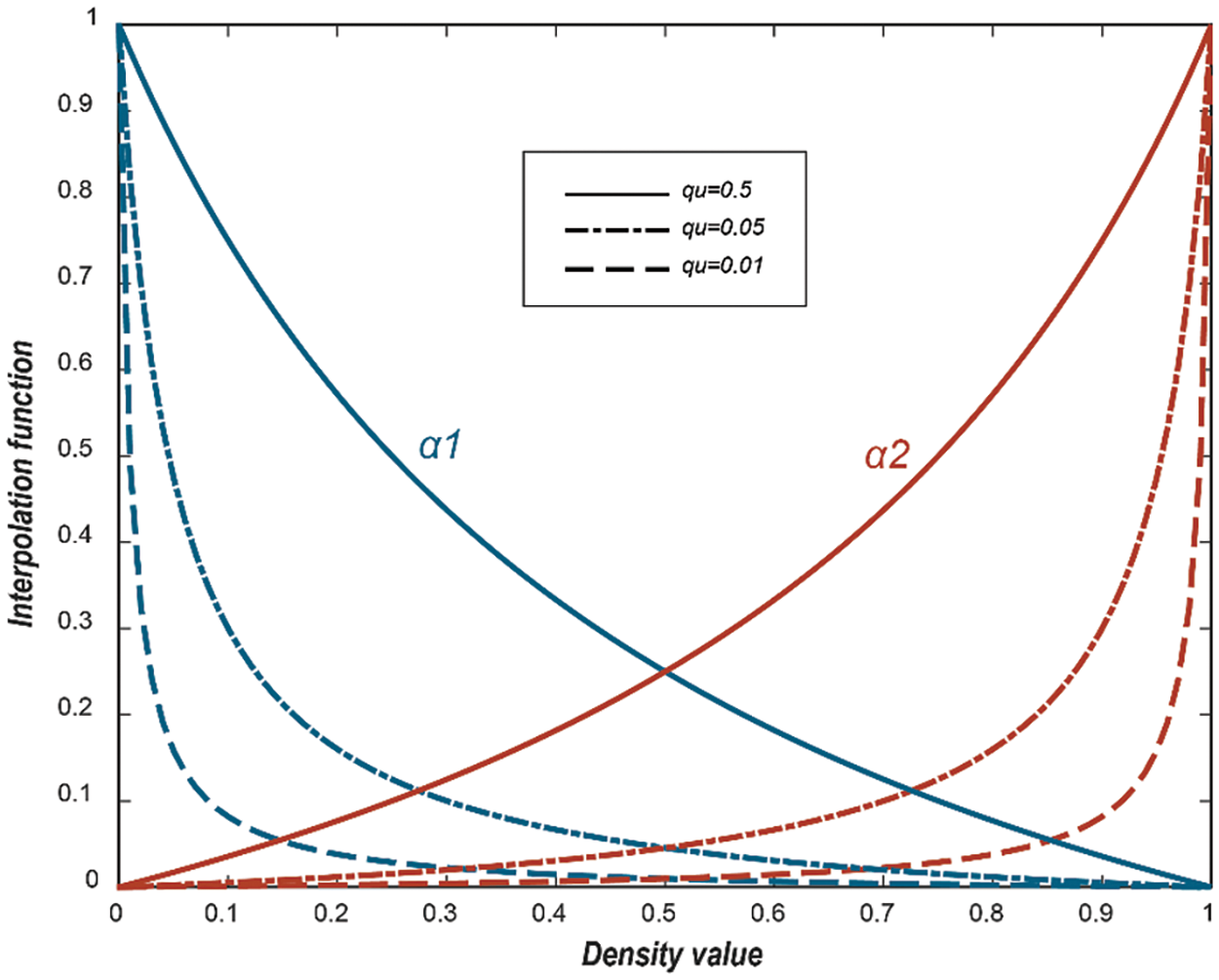
Figure 1: Interpolation curves of permeability under different qu values
After obtaining the distribution of the flow field, the two velocity fields are linearly superimposed to construct a global velocity field, leading to the formulation of the following convective heat transfer equation:
where T represents the temperature field and K is the reciprocal of the Peclet number (Pe), which is defined as follows:
where Pe is the Peclet number, Pr is the Prandtl number, ρ is the material density, cp is the material’s specific heat capacity at constant pressure, U is the characteristic velocity, l is the characteristic length, and k is the thermal conductivity of the material. The interpolation function is constructed using a Gaussian function:
where kf is the thermal conductivity of the fluid, ks is the thermal conductivity of the solid, and s is the curvature influence factor of the interpolation function, illustrated in Fig. 2.
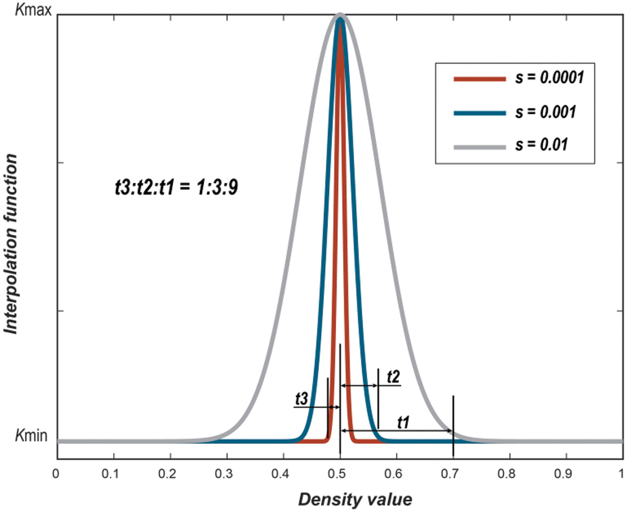
Figure 2: Interpolation curve of thermal conductivity under different s values
When s takes a more considerable value, the intermediate density units (0.3 < γ < 0.7) have higher thermal conductivity. However, in the initial optimization stages, there are many intermediate-density units. This means these units have strong heat conduction capabilities, which weakens the demand for convective heat transfer. As a result, the distribution of the flow channels becomes relatively straightforward, contradicting the original intention of the topology optimization design. Therefore, in the initial stage of the optimization design, it is necessary to consider setting the thermal conductivity of the intermediate density units to the same value as the thermal conductivity of the fluid. This can be achieved by setting a small value for s. When s is small, it can be assumed that only units within a minimal interval around a density of 0.5 are solid units. This provides greater freedom for convective heat transfer, resulting in more complex channel designs. Moreover, when s is small, the distribution of unit properties (i.e., fluid and solid differences) is more precise. In this paper, s is ultimately chosen to be 0.0001.
The physical background of the optimization is to maximize the heat transfer between the hot and cold fluids under a specific pressure drop. There are two ways to handle the pressure drop constraint. (1) The pressure drop function is a constraint in the optimization problem. (2) Setting the inlet boundary condition as a constant pressure condition. In the first method, the viscous dissipation of fluid flowing through the design domain is added to the constraint function to control the pressure drop, which not only brings more workload to the sensitivity calculation but also needs to solve more adjoint equations. The second approach constrains the pressure drop and does not require the sensitivity information of the constraint function, which can reduce computational complexity. This paper uses the second approach to constrain the pressure drop. Therefore, only the volume constraint needs to be considered. The optimization formulation in this paper is as follows:
where C is the objective function, and V is the model volume. For hot and cold fluids, the total heat exchange capacity is:
Since both density and specific heat capacity at constant pressure are constant, Eq. (7) can be simplified as the following:
In the topology optimization calculation presented in this paper, three density fields were considered, namely, the design variable density field γ (0 ≤ γ ≤ 1), Helmholtz filter [32] density field γp, and the Heaviside projected [33] density field γh, which satisfies the following relationship:
The Helmholtz equation employs a filter radius denoted as r. At the same time, the Heaviside function incorporates a projection slope denoted as β, with all projection slopes consistently set to 8 throughout this paper. Additionally, η represents the threshold value set at 0.5. Specifically, the projected density penalty tends towards 0 when the filter density is below this threshold and tends towards 1 when it exceeds this value. The utilization of the Helmholtz filter aims to mitigate the checkerboard phenomenon, while the projection of the Heaviside function serves to diminish gray units within the optimization results. The projection density, denoted as γh, is employed for computing the material thermal coefficient, objective function, sensitivity, and other relevant information.
2.4 OpenFOAM Implementation Process
This paper develops a parallel topology optimization computation program using the OpenFOAM platform and the PETSc library. Thanks to the efficiency of PETSc library functions, the program can fully leverage the parallel computing capabilities of the OpenFOAM platform for large-scale structural topology optimization calculations.
Fig. 3 illustrates the computational process of topology optimization for heat transfer between two fluid streams. The simpleFoam solver in OpenFOAM is used to solve the NS equations with certain modifications to the adjoint NS equations. The ScalarTransportFoam solver is used to solve the convective heat transfer equation and its adjoint equation with appropriate modifications.
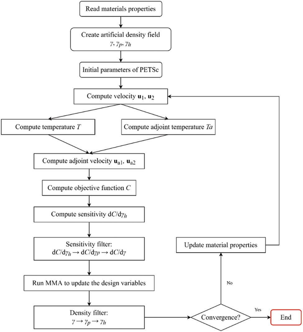
Figure 3: Two-fluid heat transfer topology optimization process
The process starts by reading the material properties, including viscosity μ, thermal conductivity k, etc. It then creates physical fields such as the artificial density field γ, velocity fields u1, u2, temperature field T, etc. The control and adjoint equations are discretized using the fvm namespace for implicit discretization of partial differential equations. The body force term in the NS equations is treated as a source term with explicit discretization.
The program first solves the NS equations. After obtaining the velocities of the two fluid streams, they are linearly combined to construct the overall velocity field for the convective heat transfer equation. Then, the convective heat transfer equation and its adjoint equation are solved. The adjoint NS equations are solved based on the obtained adjoint temperatures. Finally, sensitivity values are obtained and passed to the Moving Asymptotes Method (MMA) algorithm for updating the design variables, and the iteration process continues until convergence.
The sensitivity formulas are presented as explicit functions, allowing their direct incorporation into OpenFOAM to extract sensitivity information. It is essential to emphasize that the derived sensitivity formulas represent the derivatives of the objective function about the projected density, which is based on the Heaviside function. The reverse application of the chain rule is necessary to compute the objective function’s derivatives concerning the design variables. The obtained sensitivity information is then transformed into the MMA to update the design variables. The solver used in this study makes use of a parallel MMA algorithm that Yu et al. created within the PETSc framework [15,16]. The MPI library employed for PETSc compilation is openMPI. Following the update of the design variables, a PDE filtering process is executed.
Obtaining accurate sensitivity information is a core aspect of topology optimization because the simple algorithm is segregated, meaning the stiffness matrix is not fully assembled during the computation process. Therefore, this paper uses the continuous adjoint method to solve the sensitivity problem. The specific expressions for the adjoint equation and sensitivity formulas are provided directly, and the detailed derivation process can be found in the Appendix. This paper’s objective function is the total heat transfer, as described in Section 2.2. The symbols A and B in the objective function represent:
where
Substitute (12) into the general form of the adjoint equation and adjoint boundary conditions to obtain specific forms of sensitivity formulas, adjoint equations, and boundary conditions.
The sensitivity formula for specific forms is as follows:
The specific form of the equation is as follows:
The specific form of the accompanying boundary conditions is as follows:
1) Boundary conditions for the convection heat transfer equation
2) Boundary conditions associated with the NS equation
where hOutlet represents the hot fluid outlet, and cOutlet represents the cold fluid outlet.
OpenFOAM’s built-in classes can be used to achieve the first-type and homogeneous second-type boundary conditions. However, for special boundary conditions, custom boundary conditions need to be written by inheriting the built-in classes or using third-party libraries to implement the application of special boundary conditions. The second and third terms of Eq. (16) are applied through groovyBC in swak4Foam.
Compared with solving the adjoint control equations, which can make full use of the built-in simpleFoam solver, implementing adjoint boundary conditions at the inlet requires inheriting and deriving OpenFOAM’s fixedValueFvPatchScalarField boundary condition class. It should be noted that currently, there is no formula for adjoint pressure inlet boundary conditions in topology optimization research on fluids. This paper derives the corresponding adjoint condition for pressure inlet and provides the corresponding code in OpenFOAM to define this boundary condition. Due to space limitations, this section omits declaration definitions about derived classes. Code 1 only shows key calculation steps of the updateCoeffs() function in the adjoint pressure boundary condition class.
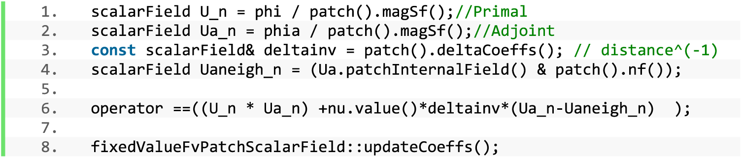
Code 1: The critical calculation steps in the boundary condition member function of the accompanying pressure inlet
4.1 A Two-Dimensional Benchmark Example
Firstly, a two-dimensional model, as shown in Fig. 4, is designed for the topology optimization study of two-fluid heat transfer. The inlet temperature of the hot fluid is set to 1, and that of the cold fluid is set to 0. It is assumed that the boundary conditions are adiabatic with no slip. The optimization objective is to maximize the heat transfer between the two fluids. The initial density value is set to 0.5. That is, the permeability of the design domain to both fluids is the same. 40,000 quadrilateral grids are used to discretize the design domain. The solution is carried out on four Intel i5-13500H CPU core computers. The optimization process takes 500 iterative steps, with an average optimization time of less than 1 s. This shows that the topology optimization program in this paper has a very high calculation speed.
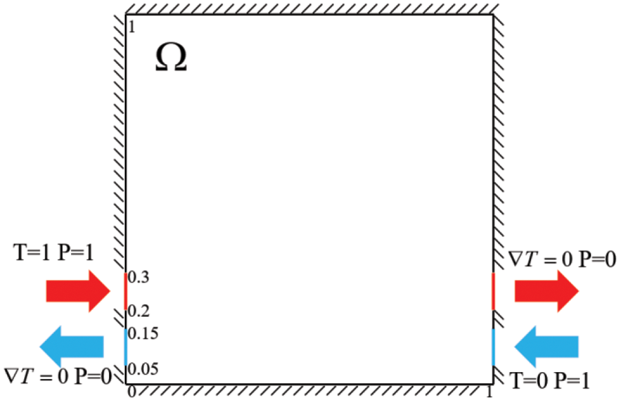
Figure 4: Two-dimensional topology optimization example
The optimized results are shown in Figs. 5 and 6. It can be observed that the optimized flow channel is Ω-like, and according to Fig. 7b, the two fluids are separated. The optimization results here preliminarily show the effectiveness of the optimization algorithm proposed in this paper, and the optimization iteration can be completed in a very short time, and each iteration takes less than one second. This provides a solid foundation for the subsequent 3D topology optimization calculation.
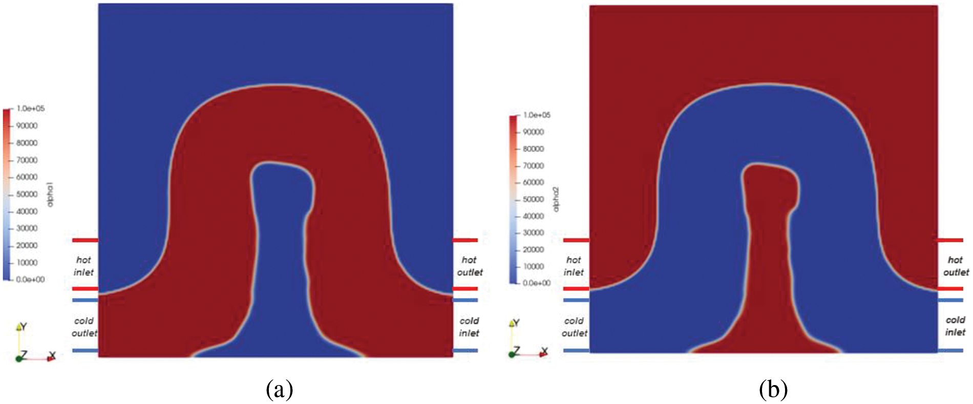
Figure 5: Two-dimensional topology optimization results and permeability distribution map under Re = 100 (a) α1 distribution map (b) α2 distribution map
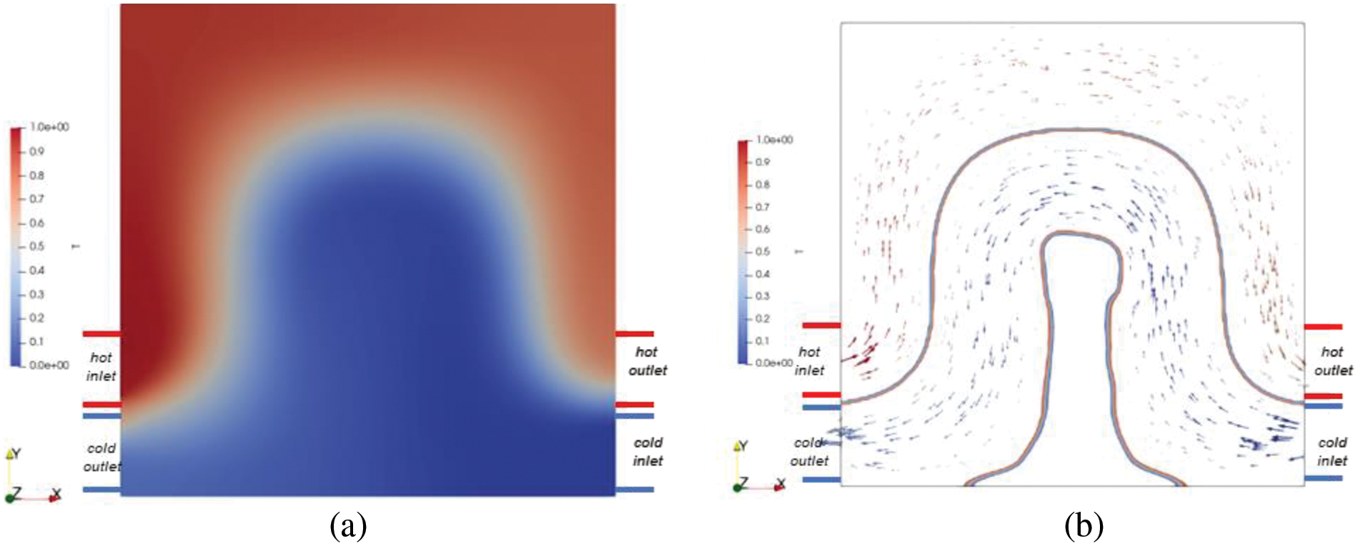
Figure 6: Two-dimensional topology optimization results: (a) temperature distribution map under Re = 100; (b) velocity distribution map
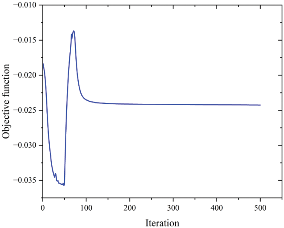
Figure 7: Graph of objective function and iteration steps under Re = 100
According to Fig. 7, the objective function initially experiences a decreasing phase, followed by a gradual increase, and then decreases until convergence. During the initial decreasing phase, the unclear flow channel structure and vigorous mixing of the two fluids gradually enhance heat transfer capability, decreasing the objective function. Subsequently, as the flow channel structure becomes clearer and separates the two fluids, heat transfer capability decreases compared to the initial stage, increasing the objective function value. Finally, with optimization progress, increasing the accessible surface area of the flow channel enhances its heat transfer capability, causing a decrease in objective function until convergence.
4.2 Three-Dimensional Benchmark Example
Subsequently, we conducted topological optimization research on three-dimensional heat exchangers under different Re. The model is shown in Fig. 8, and the characteristic dimension of Re is the length one, that is, the width of the heat exchanger. The calculation process uses dimensionless equations with corresponding boundary conditions, as shown in the figure. Based on the model’s symmetry, only half of it is calculated to reduce computational complexity. The entire model uses a regular hexahedral mesh with a total grid count of 4.86 × 10⁵, as shown in Fig. 9. Due to increased complexity, this paper used 30 HYGON 7185 physical cores for parallel computing, with an average iteration time of 30 s per step and a total of 400 steps.
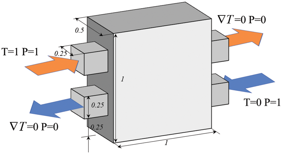
Figure 8: Three-dimensional topological optimization model of heat transfer between two fluids
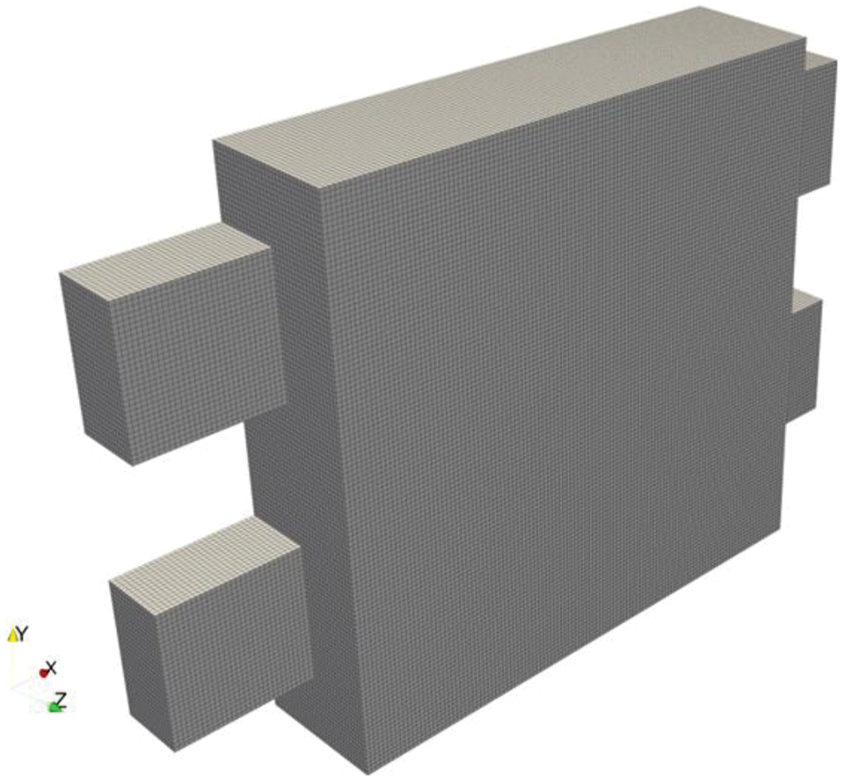
Figure 9: 486,000 standard hexahedral structured grids are used to discretize the design domain; only half of the model is discretized according to symmetry
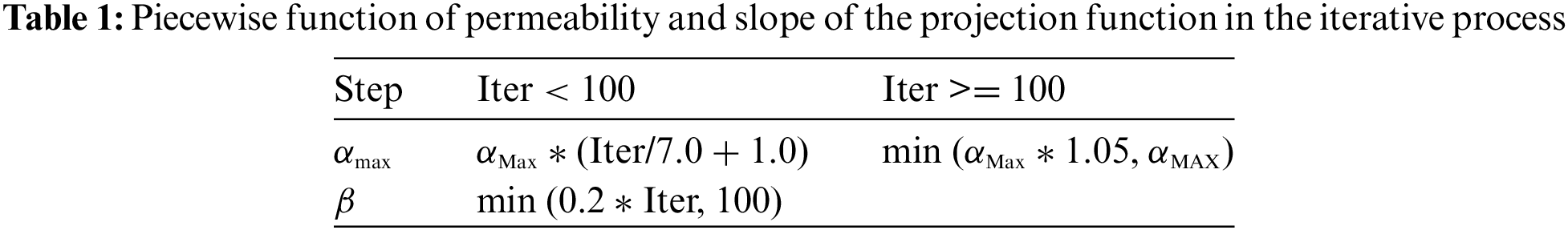
Taking Reynolds number 100 as an example, to ensure that Da is less than 10−7, it should be noted that during the initial computation stage, permeability values need to be relaxed so that flow has higher degrees of freedom and can obtain complex flow channel structures. In this paper, we set the initial inverse permeability rate at one percent of its maximum value. At the same time, in filtering operations, interpolation function slope control factors are gradually increased with the relevant parameters shown in Table 1.
Firstly, topology optimization studies were conducted for different Reynolds numbers (Re = 100, 200, 300). Fig. 10 shows the iteration history of different cross-sectional density values at Re = 300. The red part represents hot fluid, the blue part represents cold fluid, and the middle density represents solid elements. As shown in Fig. 11’s results, with the increase in Reynolds number, the flow channel structure becomes more complex, and the heat transfer area increases significantly. This enhances the convective heat transfer capability of the structure. According to control equations, when the Reynolds number increases, viscosity weakens. Thus, under a specific pressure inlet boundary condition, fluids have incredible energy to fill more complex spatial structures. At the same time, according to the results on the right side of Fig. 11, it can be seen that when Re is small, the fluid in regions far from the inlet has a smaller velocity. In contrast, as Re increases, the velocity in this region also increases. Therefore, with increasing Re, both heat transfer area and velocity increase, which improves the heat transfer capacity of the heat exchanger.
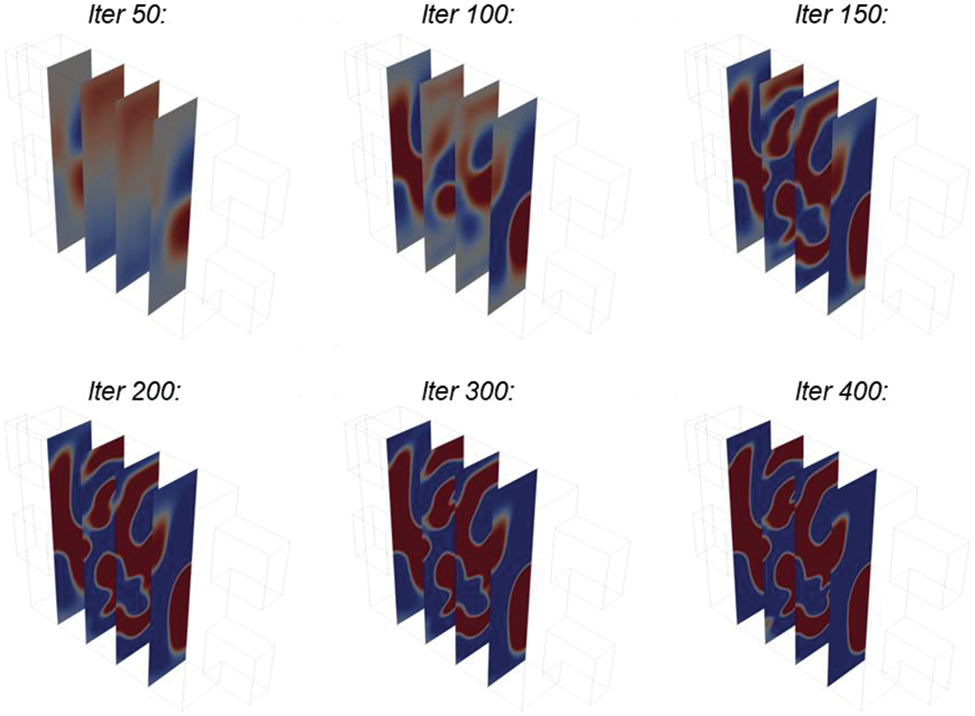
Figure 10: Iterative history of different section density values under Re = 300, where the red area represents hot fluid, and the blue area represents cold fluid
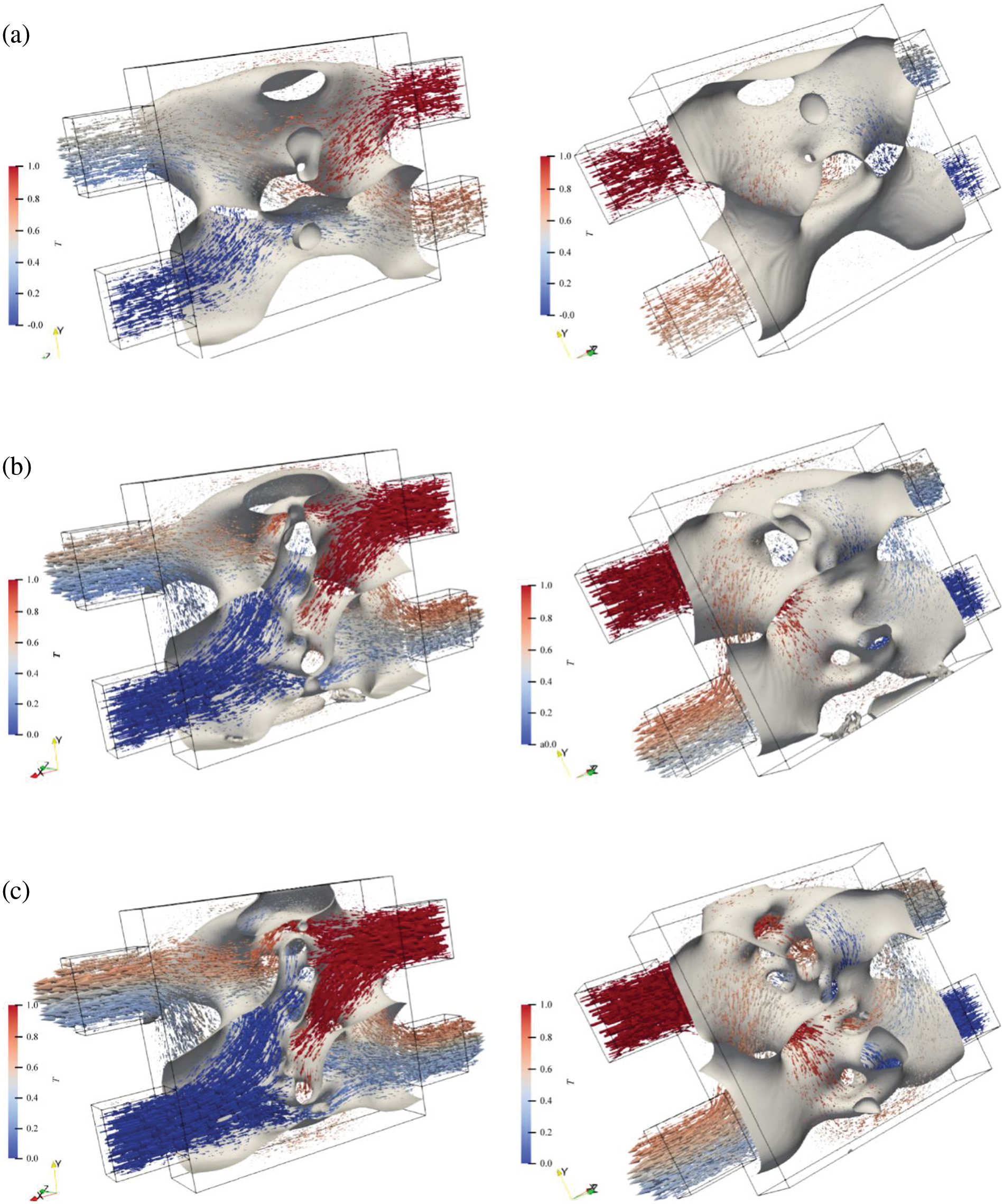
Figure 11: Optimization results under different Reynolds numbers (a) Re = 100, (b) Re = 200, (c) Re = 300
At present, structure observation reveals that there are some small diameter channels in the middle region of the structures shown in Figs. 11b and 11c. According to Bernoulli’s equation, the fluid velocity in this region is higher than that in more expansive areas. Thus, although the heat transfer area decreases here due to the increased flow rate, the overall convective heat transfer capability does not decrease.
Observing the above results, we found that the flow channel tends to narrow in the central part of the structure while presenting a broad flow channel form in areas closer to the inlet and outlet. This is because the size of the inlet and outlet of the flow channel will affect its distribution form. When the inlet and outlet sizes are significant, topology optimization results will promote adaptation between near-field flow channel sizes and inlet and outlet sizes to avoid abrupt changes in flow channel size. However, increasing dimensions will reduce fluid velocity and weaken convective heat transfer. Therefore, at the center of the structure, structural contraction increases the flow rate through narrowing channels, which enhances convective heat transfer capability.
Although such a heat exchange structure has strong heat exchange ability, its uneven distribution of structural channels could be more conducive for subsequent geometric reconstruction. Therefore, we reduced the inlet and outlet area to 1/4 of the original size and set the inlet and outlet in a diagonal position, as shown in Fig. 12. The topology optimization calculation was carried out at Re = 300, with the results illustrated below. When reducing entry/exit dimensions, the influence on the transition section from inlet/outlet to channel dimension weakens, allowing more uniform-sized channels to be distributed within the design domain.
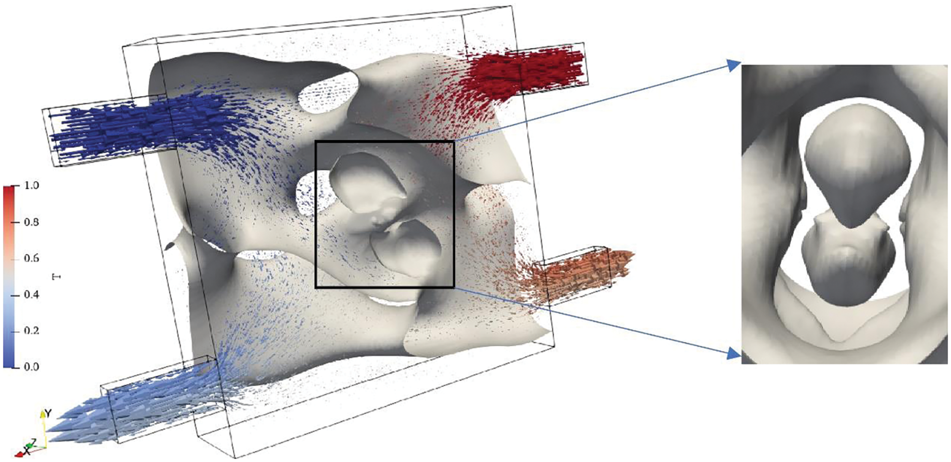
Figure 12: Three-dimensional topology optimization result after narrowing the size of the inlet and outlet
Fig. 12 illustrates that employing symmetric calculations results in a final optimized configuration featuring two isolated islands. The purpose of these islands is to facilitate the proximity of hot fluids to cold ones and augment their velocities. However, in practical scenarios, the viability of these isolated islands is compromised due to the absence of solid wall connections and separate supports. It is essential to emphasize that topology optimization outcomes are not directly implemented in actual design processes but rather undergo tailored adjustments. To exemplify, the isolated islands can be construed as floating entities. In the design phase, a streamlined component can be incorporated into the channel structure in this region to optimize convective heat transfer.
It is worth mentioning that in this example, the solid wall is often fragile. Therefore, to simplify the calculation, we assume that the thermal conductivity of the solid thin wall is equal to that of the fluid. The optimized result is shown in Fig. 13. In zones A and B of the result, although the velocity of cold fluid is small, it does not mean there is no fluid in this area. This area is filled with fluid flowing at a deficient speed. At the same time, since the overall Reynolds number is in a laminar state, there will be no vortexes in this area. Therefore, this area will not cause too much flow loss but will further promote heat exchange between two streams of fluids.
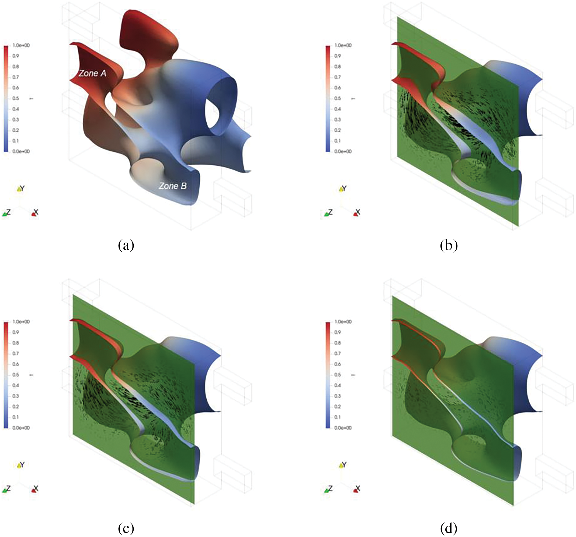
Figure 13: Topological optimization results when the thermal conductivity of fluid and solid is the same. (a) density isosurface colored by temperature; (b) velocity field distribution of z = 0.2 cross-section; (c) velocity field distribution of z = 0.22 cross-section; (d) velocity field distribution of z = 0.24 cross-section
Zone A’s fluid near the hot inflow section can be fully heated by a hot stream first; then, part of its flow mixes into the mainstream while another part transfers heat to the mainstream through conduction to provide enough heat for cold fluid. Zone B’s fluid, with a lower temperature and closer proximity to the hot outflow section, can ensure the hot stream transfers more heat to the cold one at the outlet segment. Therefore, zones A and B do not cause additional flow loss but strengthen heat exchange between the two streams.
4.3 Cross Flow Heat Exchanger Example
Next, we carry out a topology optimization design for the cubic heat exchanger with the cross-flow; according to the model’s symmetry, 416,000 hexahedral grids are used to divide the design domain. The optimized designs are shown in Fig. 14. By comparing the optimization results under different Pe, we can find that with a decrease in Pe, the number of bifurcations in the flow channel increases, and the distance between the two fluids decreases. This is because Pe represents the relative size of convection and diffusion, and the smaller the value, the weaker the convection and the stronger the diffusion. Therefore, the topology optimization results show more flow bifurcation to enhance the contribution of flow terms to heat transfer. At the same time, reducing the distance between the two fluids also reduces the heat transfer thermal resistance, which can further the heat transfer effect between the two fluids. At the same time, according to the optimization result in Fig. 15, the flow channel size is more significant in the peripheral part of the design domain than in the central area.
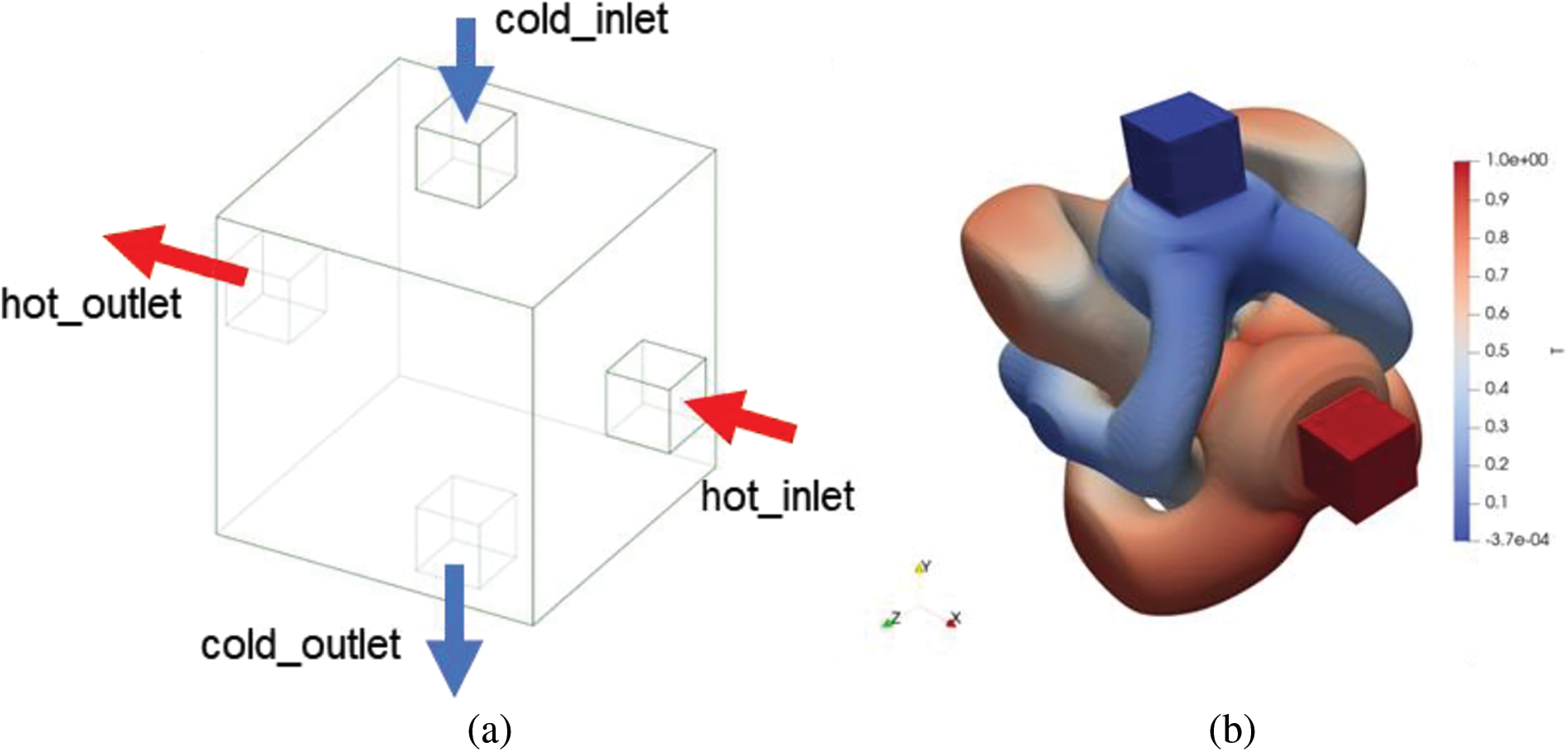
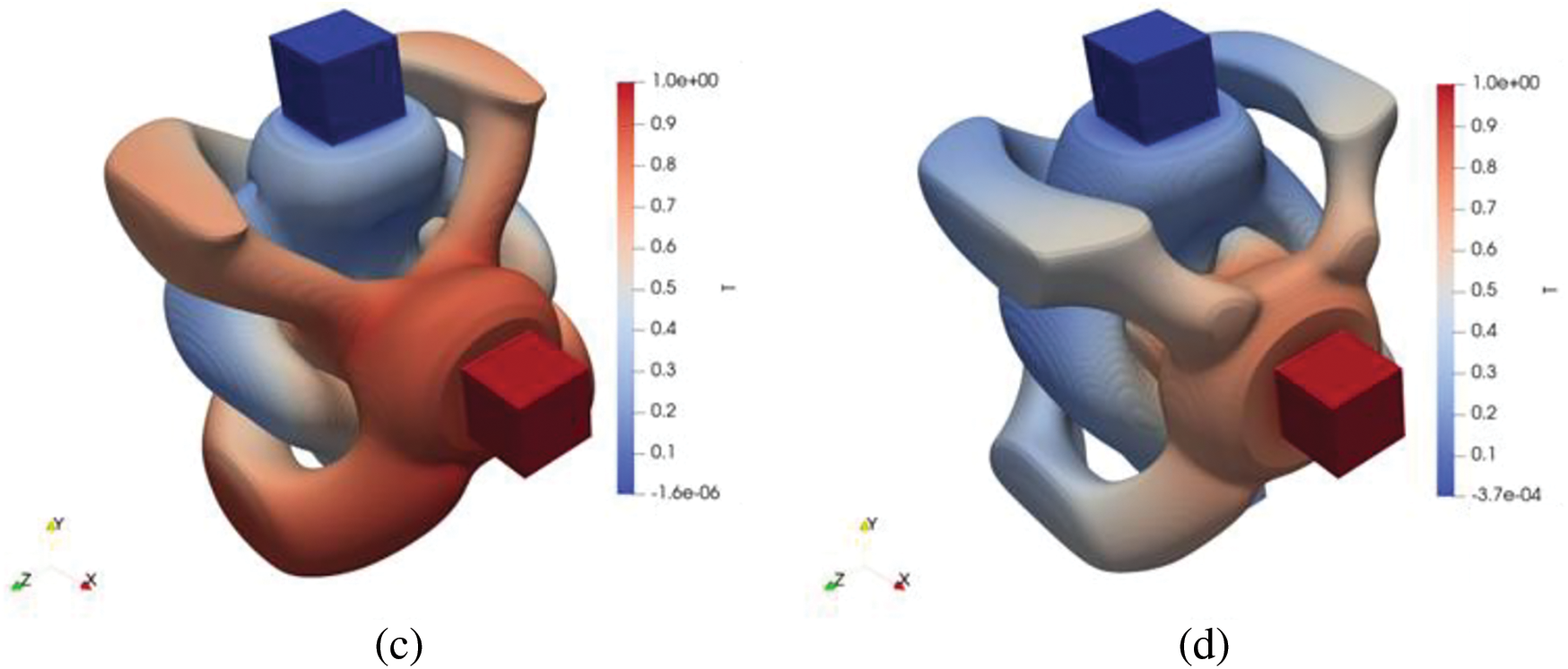
Figure 14: Topology optimization results with different Pe numbers colored by temperature (a) optimization model with cross flow (b) optimization results with Pe = 350 (c) optimization results with Pe = 700 (d) optimization results with Pe = 1400
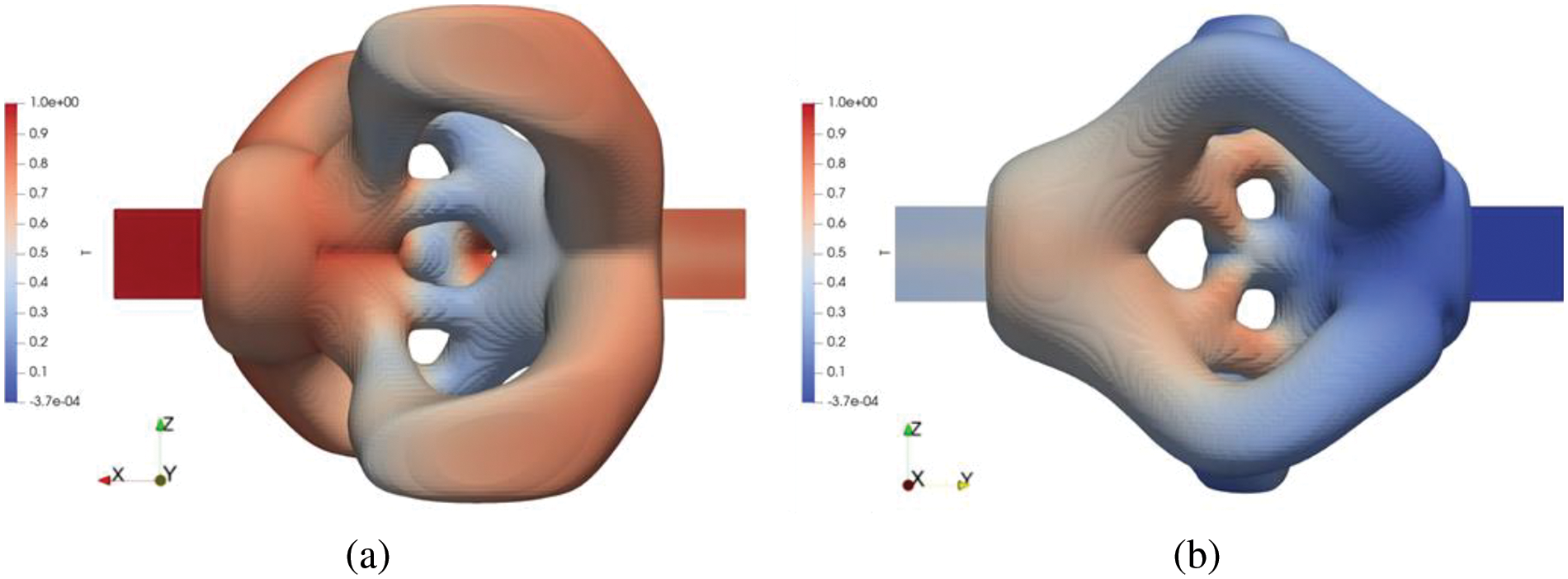
Figure 15: Distribution diagram of hot and cold fluids colored by temperature when Pe = 350 (a) +y view of hot fluid (b) +x view of cold fluid
Furthermore, 4,128,000 hexahedral grids are used to divide the design domain, and large-scale topology optimization calculations are carried out. The results are shown in Fig. 16. Observing the distribution characteristics of cold fluid is similar to the optimization results with hundreds of thousands of grids; the flow channels are distributed in the design domain in tabular form. However, under large-scale optimization, the distribution form of hot fluid channels has changed, and a new flat channel form has appeared based on tubular distribution. Under large-scale calculation, the flow channel’s characteristic size decreases, the fluid’s space in the design domain increases, and the heat exchange area between the two fluids also increases, improving the structure’s heat exchange performance. The appearance of the above new structure is also significant for carrying out large-scale topology optimization in this paper, and it also proves the effectiveness and stability of the topology optimization program written in this paper in large-scale calculation.
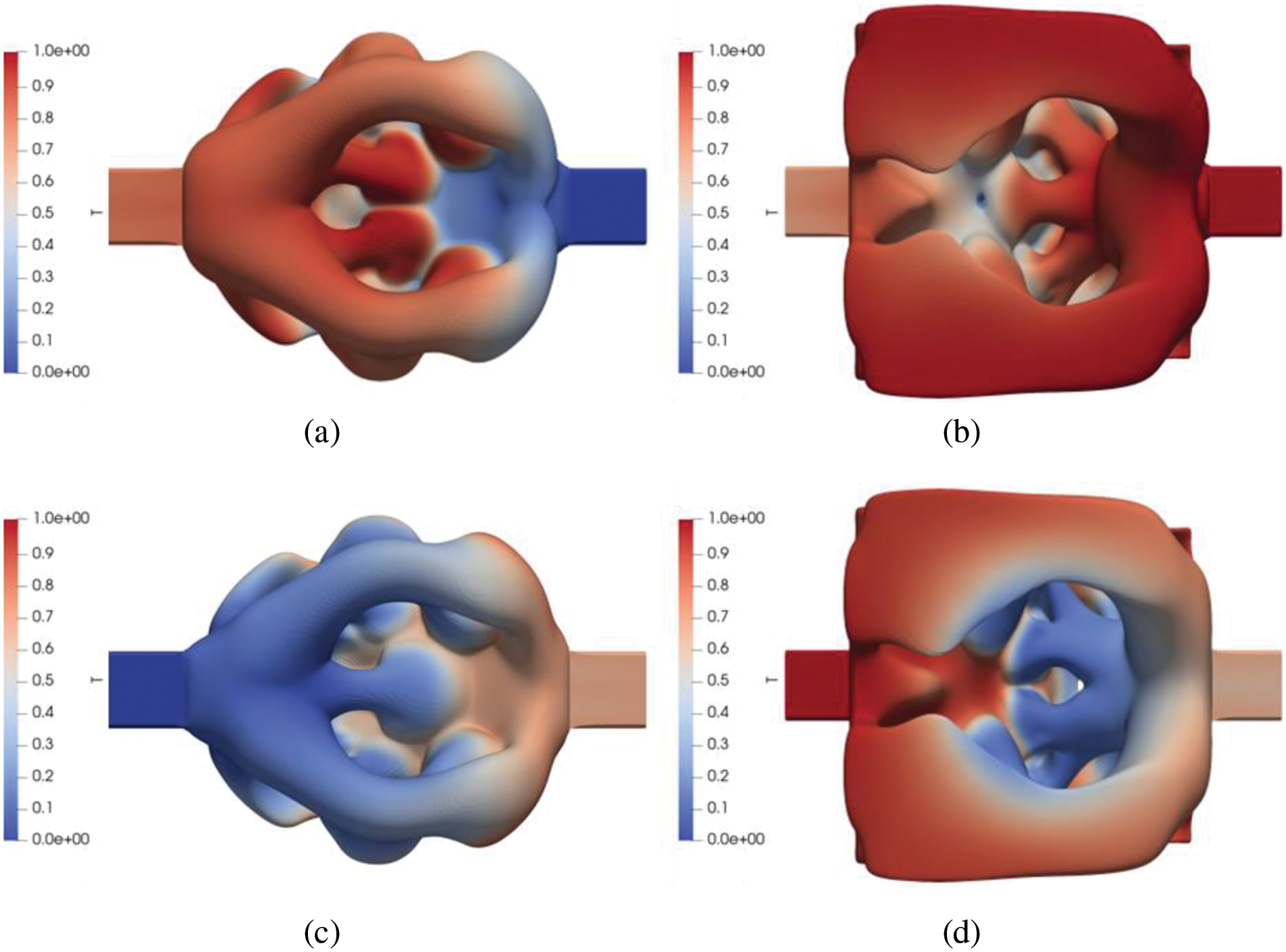
Figure 16: The results of large-scale topology optimization of 4,128,000 grids colored by temperature are (a) +x view of cold fluid, (b) +y view of hot fluid, (c) -x view of cold fluid, and (d) -y view of hot fluid, in the case of Pe = 700
This article studies two fluid heat transfer problems. Firstly, two permeability interpolation functions described by a single physical field are given, and two independent NS equations are constructed. The article discusses using the Gaussian function to construct an interpolation function for the thermal conductivity coefficient. It also analyzes the impact of different interpolation parameters on the optimization process. The study reveals that only small interpolation parameters yield reasonable optimization results.
The results of two-dimensional topology optimization preliminarily verify the effectiveness of the optimization method in this paper. At the same time, the optimization program written in this paper has a very high calculation speed. In the three-dimensional topology optimization problem, with an increase in Re, the surface area of the flow channel increases. A large-scale calculation is carried out in the topology optimization of cross-flow heat exchangers, and the optimization results in this paper also show the effectiveness and efficiency of the optimization method.
In summary, this chapter obtains topological optimization results that have guiding significance for designing new efficient heat exchangers and demonstrates their valuable contribution to our work.
Acknowledgement: None.
Funding Statement: This work was supported by the Aeronautical Science Foundation of China (Grant No. 2020Z009063001) and the Fundamental Research Funds for the Central Universities (Grant No. DUT22GF303).
Author Contributions: All authors contribute to the methodology, coding, analysis, writing and editing.
Availability of Data and Materials: All the details necessary to reproduce the results have been defined in the paper. The interested reader may contact the corresponding author for further implementation details.
Conflicts of Interest: The authors declare that they have no conflict of interest to report regarding the present study.
References
1. Bendsoe, M. P., Sigmund, O. (2003). Topology optimization: Theory, methods, and applications. Berlin: Springer Science & Business Media. [Google Scholar]
2. Bayat, M., Dong, W., Thorborg, J., Albert, C. T., Jesper, H. H. (2021). A review of multi-scale and multi-physics simulations of metal additive manufacturing processes with focus on modeling strategies. Additive Manufacturing, 47, 102278. https://doi.org/10.1016/j.addma.2021.102278 [Google Scholar] [CrossRef]
3. Cheng, K., Olhoff, N. (1982). Regularized formulation for optimal design of axisymmetric plates. International Journal of Solids and Structures, 18(2), 153–169. https://doi.org/10.1016/0020-7683(82)90023-3 [Google Scholar] [CrossRef]
4. Cheng, K., Olhoff, N. (1981). An investigation concerning optimal design of solid elastic plates. International Journal of Solids and Structures, 17(3), 305–323. https://doi.org/10.1016/0020-7683(81)90065-2 [Google Scholar] [CrossRef]
5. Bendsøe, M. P., Kikuchi, N. (1988). Generating optimal topologies in structural design using a homogenization method. Computer Methods in Applied Mechanics and Engineering, 71(2), 197–224. https://doi.org/10.1016/0045-7825(88)90086-2 [Google Scholar] [CrossRef]
6. Borrvall, T., Petersson, J. (2003). Topology optimization of fluids in Stokes flow. International Journal for Numerical Methods in Fluids, 41(1), 77–107. https://doi.org/10.1002/fld.v41:1 [Google Scholar] [CrossRef]
7. Gersborg-Hansen, A., Sigmund, O., Haber, R. B. (2005). Topology optimization of channel flow problems. Structural and Multidisciplinary Optimization, 30(3), 181–192. https://doi.org/10.1007/s00158-004-0508-7 [Google Scholar] [CrossRef]
8. Dede, E. M., Joshi, S. N., Zhou, F. (2015). Topology optimization, additive layer manufacturing, and experimental testing of an air-cooled heat sink. Journal of Mechanical Design, 137(11), 111702. [Google Scholar]
9. Yoon, G. H. (2010). Topological design of heat dissipating structure with forced convective heat transfer. Journal of Mechanical Science and Technology, 24(6), 1225–1233. https://doi.org/10.1007/s12206-010-0328-1 [Google Scholar] [CrossRef]
10. Mcconnell, C., Pingen, G. (2012). Multi-layer, pseudo 3D thermal topology optimization of heat sinks. ASME International Mechanical Engineering Congress and Exposition, pp. 2381–2392. Houston, Texas, USA. [Google Scholar]
11. Matsumori, T., Kondoh, T., Kawamoto, A., Nomura, T. (2013). Topology optimization for fluid-thermal interaction problems under constant input power. Structural and Multidisciplinary Optimization, 47(4), 571–581. https://doi.org/10.1007/s00158-013-0887-8 [Google Scholar] [CrossRef]
12. Yaji, K., Yamada, T., Kubo, S., Izui, K., Nishiwaki, S. (2015). A topology optimization method for a coupled thermal-fluid problem using level set boundary expressions. International Journal of Heat and Mass Transfer, 81, 878–888. https://doi.org/10.1016/j.ijheatmasstransfer.2014.11.005 [Google Scholar] [CrossRef]
13. Wei, P., Jiang, Z., Xu, W., Liu, Z., Deng, Y. et al. (2023). Topology optimization for steady-state Navier-Stokes flow based on parameterized level set based method. Computer Modeling in Engineering & Sciences, 136, 593–619. https://doi.org/10.32604/cmes.2023.023978 [Google Scholar] [CrossRef]
14. Baniewski-Wołłk, A., Rokicki, J. (2016). Adjoint Lattice Boltzmann for topology optimization on multi-GPU architecture. Computers & Mathematics with Applications, 71(3), 833–848. https://doi.org/10.1016/j.camwa.2015.12.043 [Google Scholar] [CrossRef]
15. Yu, M. H., Ruan, S. L., Wang, X. Y., Li, Z., Shen, C. Y. (2019). Topology optimization of thermal-fluid problem using the MMC-based approach. Structural and Multidisciplinary Optimization, 60(1), 151–165. https://doi.org/10.1007/s00158-019-02206-w [Google Scholar] [CrossRef]
16. Yu, M. H., Ruan, S. L., Gu, J. F., Ren, M. K., Li, Z. et al. (2020). Three-dimensional topology optimization of thermal-fluid-structural problems for cooling system design. Structural and Multidisciplinary Optimization, 62(6), 3347–3366. https://doi.org/10.1007/s00158-020-02731-z [Google Scholar] [CrossRef]
17. Gallorini, E., Hèlie, J., Piscaglia, F. (2023). An adjoint-based solver with adaptive mesh refinement for efficient design of coupled thermal-fluid systems. International Journal for Numerical Methods in Fluids, 95(7), 1090–1116. https://doi.org/10.1002/fld.v95.7 [Google Scholar] [CrossRef]
18. Alexandersen, J., Aage, N., Andreasen, C. S., Sigmund, O. (2014). Topology optimisation for natural convection problems. International Journal for Numerical Methods in Fluids, 76(10), 699–721. https://doi.org/10.1002/fld.v76.10 [Google Scholar] [CrossRef]
19. Coffin, P., Maute, K. (2016). A level-set method for steady-state and transient natural convection problems. Structural and Multidisciplinary Optimization, 53(5), 1047–1067. https://doi.org/10.1007/s00158-015-1377-y [Google Scholar] [CrossRef]
20. Alexandersen, J., Sigmund, O., Aage, N. (2016). Large scale three-dimensional topology optimisation of heat sinks cooled by natural convection. International Journal of Heat and Mass Transfer, 100, 876–891. https://doi.org/10.1016/j.ijheatmasstransfer.2016.05.013 [Google Scholar] [CrossRef]
21. Pollini, N., Sigmund, O., Andreasen, C. S., Alexandersen, J. (2020). A poor man’s approach for high-resolution three-dimensional topology design for natural convection problems. Advances in Engineering Software, 140, 102736. https://doi.org/10.1016/j.advengsoft.2019.102736 [Google Scholar] [CrossRef]
22. Dilgen, S. B., Dilgen, C. B., Fuhrman, D. R., Sigmund, O., Lazarov, B. S. (2018). Density based topology optimization of turbulent flow heat transfer systems. Structural and Multidisciplinary Optimization, 57, 1905–1918. https://doi.org/10.1007/s00158-018-1967-6 [Google Scholar] [CrossRef]
23. Yeranee, K., Rao, Y., Yang, L., Li, H. (2022). Enhanced thermal performance of a pin-fin cooling channel for gas turbine blade by density-based topology optimization. International Journal of Thermal Sciences, 181, 107783. https://doi.org/10.1016/j.ijthermalsci.2022.107783 [Google Scholar] [CrossRef]
24. Tawk, R., Ghannam, B., Nemer, M. (2019). Topology optimization of heat and mass transfer problems in two fluids—One solid domains. Numerical Heat Transfer, Part B: Fundamentals, 76(3), 130–151. https://doi.org/10.1080/10407790.2019.1644919 [Google Scholar] [CrossRef]
25. Kobayashi, H., Yaji, K., Yamasaki, S., Fujita, K. (2021). Topology design of two-fluid heat exchange. Structural and Multidisciplinary Optimization, 63(2), 821–834. https://doi.org/10.1007/s00158-020-02736-8 [Google Scholar] [CrossRef]
26. Høghøj, L. C., Nørhave, D. R., Alexandersen, J., Sigmund, O., Andreasen, C. (2020). Topology optimization of two fluid heat exchangers. International Journal of Heat and Mass Transfer, 163, 120543. https://doi.org/10.1016/j.ijheatmasstransfer.2020.120543 [Google Scholar] [CrossRef]
27. Feppon, F., Allaire, G., Dapogny, C., Jolivet, P. (2021). Body-fitted topology optimization of 2D and 3D fluid-to-fluid heat exchangers. Computer Methods in Applied Mechanics and Engineering, 376, 113638. https://doi.org/10.1016/j.cma.2020.113638 [Google Scholar] [CrossRef]
28. Galanos, N., Papoutsis-Kiachagias, E. M., Giannakoglou, K. C., Kondo, Y., Tanimoto, K. (2022). Synergistic use of adjoint-based topology and shape optimization for the design of Bi-fluid heat exchangers. Structural and Multidisciplinary Optimization, 65(9), 245. https://doi.org/10.1007/s00158-022-03330-w [Google Scholar] [CrossRef]
29. Wang, Y. G., Li, X. Q., Long, K., Wei, P. (2023). Open-source codes of topology optimization: A summary for beginners to start their research. Computer Modeling in Engineering & Sciences, 137(1), 1–34. https://doi.org/10.32604/cmes.2023.027603 [Google Scholar] [CrossRef]
30. Darwish, M., Moukalled, F. (2021). The finite volume method in computational fluid dynamics: An advanced introduction with OpenFOAM® and Matlab®. Cham: Springer. [Google Scholar]
31. Aage, N., Andreassen, E., Lazarov, B. S. (2015). Topology optimization using PETSc: An easy-to-use, fully parallel, open source topology optimization framework. Structural and Multidisciplinary Optimization, 51, 565–572. https://doi.org/10.1007/s00158-014-1157-0 [Google Scholar] [CrossRef]
32. Lazarov, B. S., Sigmund, O. (2011). Filters in topology optimization based on Helmholtz-type differential equations. International Journal for Numerical Methods in Engineering, 86(6), 765–781. https://doi.org/10.1002/nme.v86.6 [Google Scholar] [CrossRef]
33. Wang, F., Lazarov, B. S., Sigmund, O. (2011). On projection methods, convergence and robust formulations in topology optimization. Structural and Multidisciplinary Optimization, 43, 767–784. https://doi.org/10.1007/s00158-010-0602-y [Google Scholar] [CrossRef]
Appendix
This paper uses the continuous adjoint method to solve the sensitivity problem. Firstly, the augmented Lagrangian function is constructed:
where
The domain integral term in the augmented Lagrange function is integrated by parts:
According to the KKT condition of optimization under the constraint of partial differential equations, the Gato derivative needs to be equal to 0; the formula in brackets in (19) is 0 and has the following formula:
where
Eq. (22) is transformed into the following formula:
For a general objective function, its Gato derivative with respect to variables is as follows:
The adjoint equation is obtained as follows:
Adjoint boundary condition is:
Cite This Article
 Copyright © 2024 The Author(s). Published by Tech Science Press.
This work is licensed under a Creative Commons Attribution 4.0 International License , which permits unrestricted use, distribution, and reproduction in any medium, provided the original work is properly cited.
 Downloads
 Citation Tools