
 Submit a Paper
 Propose a Special lssue
 Open Access
ARTICLE

Direct Pointwise Comparison of FE Predictions to StereoDIC Measurements: Developments and Validation Using Double Edge-Notched Tensile Specimen
1 Department of Mechanical Engineering, University of South Carolina, Columbia, SC, 29208, USA
2 Correlated Solutions Incorporated, 121 Dutchman Blvd, Columbia, SC, 29063, USA
* Corresponding Author: Michael A. Sutton. Email:
Computer Modeling in Engineering & Sciences 2024, 140(2), 1263-1298. https://doi.org/10.32604/cmes.2024.048743
Received 17 December 2023; Accepted 12 March 2024; Issue published 20 May 2024
 View Full Text
 Download PDF
Abstract
To compare finite element analysis (FEA) predictions and stereovision digital image correlation (StereoDIC) strain measurements at the same spatial positions throughout a region of interest, a field comparison procedure is developed. The procedure includes (a) conversion of the finite element data into a triangular mesh, (b) selection of a common coordinate system, (c) determination of the rigid body transformation to place both measurements and FEA data in the same system and (d) interpolation of the FEA nodal information to the same spatial locations as the StereoDIC measurements using barycentric coordinates. For an aluminum Al-6061 double edge notched tensile specimen, FEA results are obtained using both the von Mises isotropic yield criterion and Hill’s quadratic anisotropic yield criterion, with the unknown Hill model parameters determined using full-field specimen strain measurements for the nominally plane stress specimen. Using Hill’s quadratic anisotropic yield criterion, the point-by-point comparison of experimentally based full-field strains and stresses to finite element predictions are shown to be in excellent agreement, confirming the effectiveness of the field comparison process.Keywords
Nomenclature
| DEN | Double edge notched tensile specimen |
| FEA | Finite element analysis |
| FE | Finite element |
| 3D | Three-dimensional |
| MTS | Material Test Systems Corporation |
| Equivalent stress (FL−2) | |
| Yield stress (FL−2) | |
| σij | Components of the stress tensor (FL−2) |
| VTK | Visualization ToolKit, an open-source, freely available software system for 3D computer graphics, modeling, image processing, volume rendering, scientific visualization, and 2D plotting |
| VTP | Visualization Toolkit Polygonal Data file format for storing VTK surface models (polydata) |
| Polydata | Surface mesh that consists of data arrays in points, cells, or in the dataset itself. The algorithm has special traversal and data manipulation methods to process data efficiently |
| XML | Extensible Markup Language used to define and store data in a shareable manner. |
| Open3D | Library of open access programs for coordinate transformation and modification of 3D data sets |
| Python | Interpreted, object-oriented, high-level programming language with dynamic semantics. Its high-level built in data structures, combined with dynamic typing and dynamic binding, make it very attractive for rapid application development. |
| MTS 810 | Electromechanical tension test frame manufactured by MTS Corporation |
| E | Young’s modulus or Modulus of Elasticity (FL−2) |
| ν | Poisson’s ratio |
| σaxial | Engineering stress obtained from uniaxial tensile experiment (FL−2) |
| εaxial | Engineering strain obtained from uniaxial tensile experiment |
| σ, σtrue | True stress obtained from uniaxial tensile experiment (FL−2) |
| ε, εtrue | True strain obtained from uniaxial tensile experiment |
| εT | Total equivalent strain at any point, as defined in Eq. (5) |
| Elastic strain components | |
| Plastic strain components | |
| ΔE12, ΔE23 | Percent difference in εT at several nodes when comparing FE predictions from mesh 2 to mesh 1 and mesh 3 to mesh 2, respectively, as defined in Eq. (4) |
| LED | Light Emitting DIode light used to illuminate specimen during imaging |
| Components of the incremental plastic strain tensor | |
| Plastic multiplier | |
| Plastic potential | |
| FPFH | Fast Point Feature Histogram |
| ICP | Iterative Closest Point |
| K-D Tree | Binary search tree that organizes points in a K-Dimensional space with each node in the tree representing a K-Dimensional point |
| Rij | Components of the orthonormal rigid body rotation tensor |
| 1, 2, 3 | Cartesian coordinate system |
| Directional yield stress ratios | |
| Δεij | εij exp – εij mod |
| εij exp | Experimentally measured strain components |
| εij mod | Model-predicted strain components |
| σij exp | Stress components obtained using measured strains and a yield criterion (FL−2) |
| σij mod | Model predicted stress components using the same yield criterion as employed for σij exp (FL−2) |
| Δσij | σij exp – σij mod (FL−2) |
| ∂ui/∂xj | Gradients of the displacement vector components |
| ti | Translation vector from model to experimental coordinate system (L) |
| DIC | Digital Image Correlation |
| 2D-DIC | Two-dimensional DIC |
| StereoDIC | Stereo DIC |
| VIC-3D | Correlated Solutions software for StereoDIC analysis of images |
| VIC-3D.OUT | Output file for VIC-3D software |
| VicPy | Correlated Solutions Python library and interpreter |
| ANSYS | Commercial FE software package |
| SOLID186 | ANSYS finite element type used in this study |
| ABAQUS | Commercial FE software package |
| Al6061-T6 | Aluminum with 6061 designating its constituents and T6 designating temper |
| Q | Arbitrary point on the specimen that is imaged by both stereo cameras |
| P1, P2 | Pinhole locations for camera 1 and camera 2 in a stereovision system that is modeled as a pinhole camera. |
| λ1, λ2 | Scale factors for cameras 1 and 2 converting pixels to metric units (L/pixel) |
| f 1, f 2 | Distances from camera 1 and 2 pinholes along the optical axis to the center of image sensor plane, respectively (pixels). |
| Cx1, Cy1 | Location of the center of camera 1 image sensor plane (pixels) |
| Cx2, Cy2 | Location of the center of camera 2 image sensor plane (pixels) |
| X, Y, Z | Global coordinate system |
| x, y, z | Pinhole camera system, with separate systems for each camera |
| Xs, Ys | Sensor plane coordinate system, with separate systems for each camera sensor plane |
| xs, ys | Sensor coordinates of Q in image, different sensor locations for each camera (pixels) |
| Tx, Ty, Tz | Components of baseline position vector between P1 and P2 in Fig. 6 (L) |
| α, β, γ | Three angles relating x,y,z for camera 1 to x,y,z for camera 2 in Fig. 6 (°) |
| κ1, κ2 | Radial lens distortion correction factors for r3 and r5 (L−2 and L−4 units, respectively) |
| µε | Strain x 10−6 |
| pixel | Picture element or an individual sensor in the camera sensor plane |
| SD | Standard Deviation |
| IRIS | Graphical interface within VIC-3D version 9 and higher software packages |
| VIC-Snap | Correlated Solutions image acquisition and synchronization software |
| U,V,W | Displacements of specimen in x, y, z system shown in Fig. 9. Same x, y, z directions are used in Figs. 8–10, 12, 13and 17(L) |
| Kt | Stress concentration factor |
| Kf | Fatigue factor |
| q | Notch sensitivity factor |
| HAY | Hill’s quadratic Anisotropic Yield criterion |
| F,G,H,L,M,N | Parameters for the HAY criterion defined in Eqs. (7) and (8) |
| RSij | Ratios of yield stresses due to σij with the uniaxial yield stress, σy |
| σyyfar field | Uniaxial tensile stress applied by mechanical test system (FL−2) |
| r | Vector between two spatial points that is used in Appendix A (L) |
| n | Normal vector for a surface as used in Appendix A |
For complex problems, finite element (FE) simulations are integral to predicting physical phenomena, with the accuracy of FE analysis directly dependent on various factors, including boundary conditions, loading, and material properties. Analyses are generally paired with experiments to validate model predictions. Kobayashi [1] wrote one of the earliest such articles in 1983. In his paper, the author designated the methodology as a hybrid experimental-computational approach. As he noted, the concept had been around since the mid-century but became more popular in the 1970 s with increasing computer speeds and improved numerical analysis software. This was particularly true in experimental mechanics. As noted by Kobayashi, growth of the full-field moire' method provided investigators with the ability to measure interior and boundary displacements on nominally planar specimens during mechanical loading. The boundary measurements could then be used as input in the hybrid approach to more accurately predict specimen response in real-world applications. McNeill et al. [2] followed this work by developing boundary element software, performing baseline studies applying boundary displacements with Gaussian noise. The least squares approach was used to quantify the effect of noise on boundary and interior stress predictions. Their results indicated that interior stresses at least five boundary element lengths from the boundary were predicted accurately. In the new millennium, investigators [3] used a hybrid experimental-numerical procedure with a twist. In their studies, the authors extracted a three-dimensional sub-region around a crack to perform sub-region FE analysis. Using a rigid normal assumption to determine deformations on the back surface while measuring data only on the front surface using stereo imaging and StereoDIC for image analysis, the authors smoothed the measured boundary displacements for input to the FE program. Results from the studies demonstrated excellent agreement between FE predictions and measurements on both the sub-region boundary and at interior points, provided that (a) measurement locations and FE nodes where data is input are at the same spatial positions and (b) material properties are accurately estimated prior to performing the simulations.
İplikçioğlu et al. [4] performed studies with dental implants, comparing non-linear FE predictions of vertical and transverse strains to strain gage measurements bonded to an implant-abutment complex that was loaded vertically and transversely. Noting that the predicted “averaged strains” under transverse loading did not agree with gage measurements, the authors indicated this was most likely due to factors such as geometric or material property differences. In a more recent study, the authors [5] used both strain gages and DIC to measure strains on a welded specimen undergoing 3-point bending. Though the gage and local DIC results agreed, FE predictions did not agree with the measurements, the authors noting several factors including (a) geometric differences in the actual weldment geometry vs. the model rendition and (b) the material properties used in the simulations which did not include variations expected in the weld. As part of his work with the Indian Space Center, Pany [6] performed FE and membrane theory analysis for a thin-wall pressure vessel and compared predictions to a single strain gage measurement. Noting that the predicted hoop strains deviated from the strain gauge measurement, the author measured the profile of the as-manufactured shape of the cylindrical shell in the region where the strain gauge was mounted. Using the updated shape, the FE prediction of the hoop strain using the modified geometry was shown to be closer to the hoop strain measurement, with the modified shape introducing bending stresses/strains that were not included in previous FE and membrane theory predictions. In a related study, Pany [7] again combined strain gage measurements with FE simulations for a tank containing a long seam joint.
An elegant theoretical development involving both DIC measurements and FE simulations was proposed [8]. In their work, the authors consider the measured displacement fields as inherently a function of the underlying constitutive formulation. Since DIC measures the total displacement, and thus includes rigid body motions, elastic components, and plastic components, the authors proposed the use of an anelastic (time dependent) component to define an auxiliary problem to be solved so that the constitutive properties could be determined in each region. Conceptually complex, the authors developed their own software and used it to demonstrate the procedure with simulated nodal data for several 2D problems, concluding that the overall approach for determining local properties, and hence local stresses, is effective.
In another related study, the authors [9] used 2D-DIC to measure surface displacement fields on uniaxial tension and simple shear specimens, performing FE simulations for comparison to the measurements. Through differentiation of the measured displacements, the authors estimated the in-plane strains and used an elasto-plastic material model with independently determined material properties to predict the applied forces. The authors then indicated their FE model estimates for the applied boundary forces deviated substantially from the measured forces, while the measured forces were in good agreement with values estimated using only the DIC measurements and material properties.
To determine whether high magnification imaging could be used with 2D-DIC to estimate residual stresses during hole drilling, investigators [10] developed a method to correct 2D-DIC measurements for the effects of rigid body camera motion that occurred during the hole drilling process. Using established theoretical relationships between the changes in measured displacement and the residual stresses that are released during hole drilling, the authors indicated that stress errors on the order of 7% were obtained from one experiment, though no pointwise comparisons of 2D-DIC measurements and full-field model predictions were shown. A previous study related to this was performed by Torabi et al. [11] using 2D-DIC to obtain in-plane surface displacements in the vicinity of a V-shaped notch. Showing global contours of measured full-field displacements and FE predictions of displacements, the authors used least squares to optimally determine parameters in an analytic solution in the vicinity of the notch, indicating that good agreement was obtained. However, no pointwise comparisons of the FE and experimental data were shown.
He et al. [12] manufactured a cube specimen that is 50% aggregate and 50% mortar, subjecting the specimen to compressive loading. Using a scanning electron microscope to acquire high magnification images and 2D-DIC to analyze the images, the authors obtained the compressive strain field. For their uniaxial compressive loading case, the authors combined the compressive strain measurements with uniaxial stress metrics to estimate the evolution of compressive modulus as one moves from the interface into the mortar.
To assess the accuracy of 2D-DIC measurements for planar specimens, investigators [13] performed both tensile experiments and FE simulations on planar specimens with a range of geometric cutouts. By globally comparing strain contours obtained by FE simulations and 2D-DIC measurements, the authors concluded that there was “fairly good” agreement between the predictions and FE simulations, though no pointwise comparisons were shown. In addition, the authors computed the local stress concentration factor, Kt, and fatigue factor, Kf, near the cutouts for their material system using 2D-DIC results and FE simulations, concluding that the theoretical models did not agree with the 2D-DIC based results for Kt. Careful inspection of the FE and 2D-DIC strain fields near the cutouts where Kt was estimated clearly show significant differences near the notches that are most likely the reason for the observed differences, though no pointwise comparisons were shown to quantify the differences.
Yasmeen et al. [14] performed a series of tension and torsion experiments on precision machined, thin-walled aluminum specimens extracted at different angles from a rolled plate, with surface strains obtained using StereoDIC. Employing both an isotropic yield criterion [15] and a six-parameter anisotropic yield criterion [16], the authors compared the measured and predicted average total surface shear strain vs. average surface shear stress, with experimental data in good agreement with Barlat model predictions (+/−5%) but with larger differences when using the von Mises model (up to 25% difference).
In the enclosed work, the authors present a complete field comparison procedure developed to co-register FEA predictions and experimental data at the same spatial positions throughout a region of interest, providing a direct way to assess the level of agreement at each spatial location. The authors demonstrate the methodology using a nominally planar, double edge notched (DEN) aluminum specimen that is subjected to far-field tensile loads, showing the importance of the pointwise comparison procedure for accurate assessment of model and experimental agreement. Sections 2.1–2.3 detail the field comparison and interpolation methodologies developed for field comparison of predictions and measurements at the same spatial locations. Sections 3.1–3.7 describe the experimental studies and the StereoDIC method used to obtain full-field displacements and strains, showing full-field strains at selected load levels in Section 3.8. Sections 4.1 and 4.2 describe the FE model. Section 4.3 details the von Mises isotropic yield criterion and Hill’s quadratic anisotropic yield criterion (HAY) [17] used in this study. Sections 5.1 and 5.2 present results from the computational studies along with comparisons of StereoDIC experimental measurements to full-field FE predictions using the von Mises and HAY criteria, respectively. To highlight the importance of point-by-point comparisons when assessing the level of agreement between measurements and predictions, line plots comparing FE predictions and StereoDIC measurements of the strains εxx and εyy are also shown in Section 5.1. When using the HAY criterion, Section 5.3 compares FE stress predictions to StereoDIC measurement-based stresses at all points on the specimen, and Section 5.4 compares notch tip parameters obtained using both FE stress predictions to StereoDIC measurement-based stresses. Section 6 provides a discussion of the findings. Section 7 briefly describes the potential long-term implications and Section 8 highlights conclusions for the work.
Conceptually, there are three ways in which the measurements and predictions can be compared at common spatial locations.
(a) Transform data at measurement locations into values at FE nodal locations.
(b) Transform both experimental data and model predictions into values at pre-specified locations using a specific coordinate system.
(c) Transform model predictions at nodal points into predictions at measurement locations.
The transformation in (a) is useful when importing measurements to an FE code and performing a form of hybrid analysis such as the ones noted in [1,2,5] that use experimental data in the solution process. The transformation in (b) is important in applications where data is needed (b-1) at specific locations that may not coincide with FE nodes or (b-2) in a specific coordinate system (e.g., uniform Cartesian mesh, cylindrical coordinate system) for comparison to a theoretical construct. The transformation in (c) is the one described in the enclosed study and discussed in detail in Sections 2.1–2.3.
2.1 Methodology for Point-by-Point Comparison of FE Predictions and Experimental Measurements at the Same Spatial Locations
A flowchart for the methodology developed by the authors to obtain point-by-point field comparisons of the measurements and FE predictions at the same spatial locations in the measurement coordinate system and quantitatively assess the level of agreement is shown schematically in Fig. 1. As shown in Fig. 1, there are several steps in the field comparison process. For interpolation purposes, the authors developed algorithms to identify the FE model surface corresponding to the StereoDIC measurement. Using the scripting interface within ANSYS and ABAQUS, which provides direct access to the solution environment, the element faces on the FE surface are converted into triangular elements, as some elements may contain quadrilateral faces. During this process, the authors retrieved mesh information (i.e., nodal locations, mesh connectivity and coordinate system) and computational results including displacements, strains, and stresses for future interpolation.
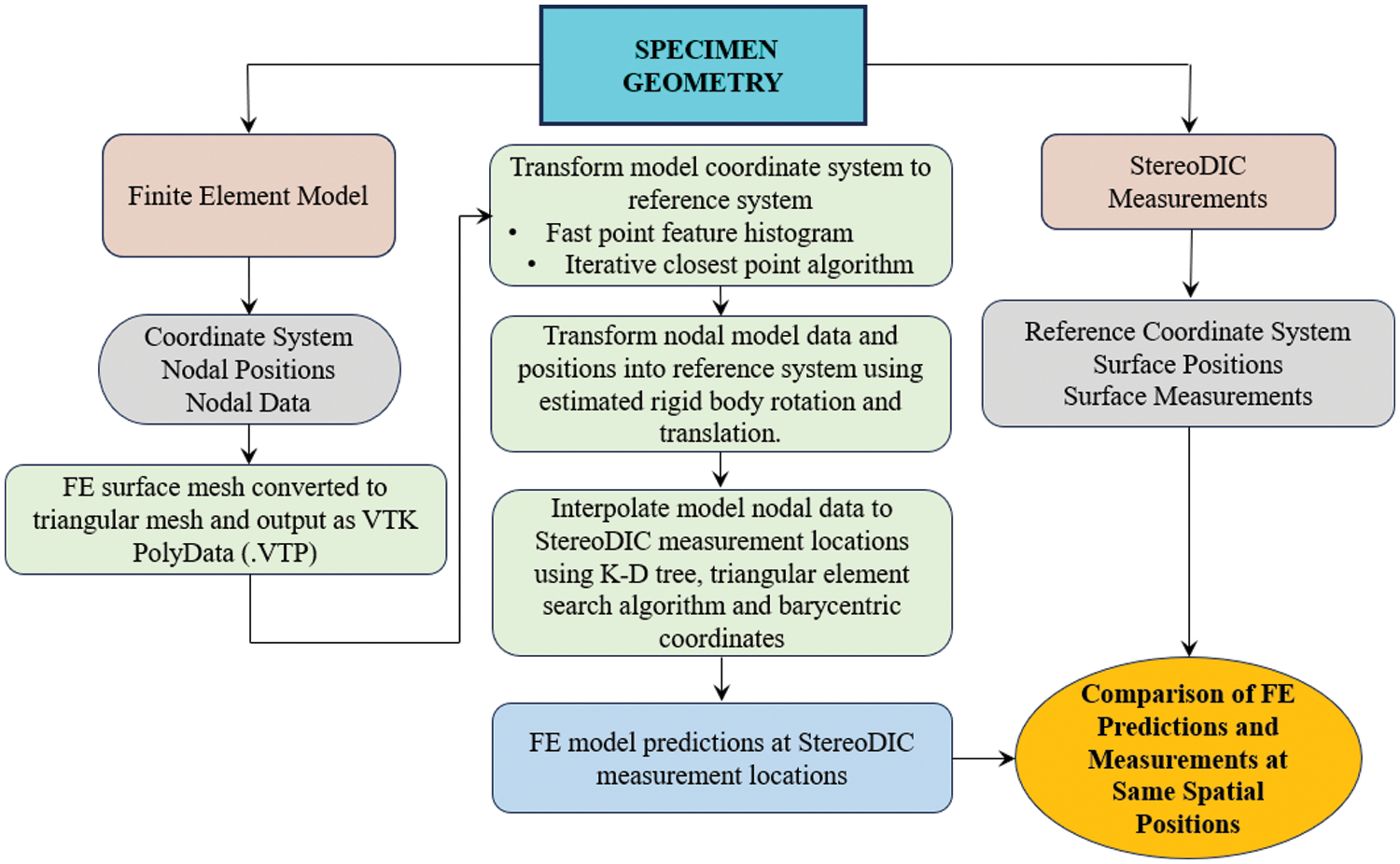
Figure 1: Flowchart for full-field transformation of model predictions at nodal points into model predictions at measurement locations for direct, point-by-point comparison
After triangularization of the mesh and extraction of the computational results, the information is then output as a VTK polydata object and stored as a .vtp file. Since external Python libraries are not accessible within either the ABAQUS or ANSYS scripting interfaces, the .vtp file is manually written in an appropriate XML syntax structure as specified within VTK documentation. After conversion to the .vtp format, VTK interpreters access details such as nodes, element connectivity, field variables, etc., for rendering and data processing purposes.
To convert the model coordinate system into the measurement coordinate system, feature identification algorithms are used to match selected model positions with corresponding measurement locations and obtain the required rigid body translation and rotations. Next, rigid body motions are used to convert all nodal locations and data (e.g., strains, displacements) into the measurement coordinate system. In the final steps, a combination of algorithms is used with the triangular mesh and barycentric coordinates to obtain FE data at all measurement locations for comparison at the same spatial positions. Details for the coordinate transformation process that underpins the field comparison process are given in Section 2.2.
As shown in Fig. 1, the coordinate transformation between the model system and the measurement system is an integral part of the comparison process. There are several approaches that can be used to transform the model coordinate system into the measurement coordinate system, or vice versa. A few of the common approaches are discussed in the following sections, with some of the approaches readily adapted to allow manual user determination and adjustment of transformation parameters.
2.2.1 Feature Extraction and Identification
To obtain the 3D position of a point/feature on the physical specimen that is in correspondence with a model location, a common approach is to identify the point/feature visually in both stereo images. For specimens with existing features (e.g., corners, notches, interfaces), identifying the pixel locations of the common feature in both cameras in a stereovision system is sufficient to obtain the three-dimensional position when using a calibrated stereovision system; additional details for a typical two-camera stereovision system are provided in Section 3.5. After determining the metric translation required to transform the corresponding feature location in the model into the measurement system, the process is repeated for several non-colinear points in both the measurement and model systems and used to define the components of rigid body rotation between the two systems. Since there are inevitable inaccuracies when determining the position of a feature in an image (typical estimates are +/−1 pixel in each image plane), using multiple features to define an optimal rigid body rotation matrix is recommended. Once the rigid body translation vector and rotation matrix are determined, all model locations are transformed into the measurement coordinate system, as discussed in Section 2.3.1.
For applications where natural surface features are not present, the application of surface markers is another option. Typically, circular markers are placed on the specimen surface to take advantage of their natural symmetry and optimally determine the pixel location of the marker center in both cameras. Once the marker locations are identified in both stereo cameras, the remainder of the process to define the Transformation between coordinate systems is the same as outlined in the previous section, with placement of multiple markers improving accuracy of the transformation parameters.
A more sophisticated approach utilizes concepts from the computer vision and computer graphics communities to co-register related, transformed, data sets. In this approach, the 3D nodal data from the FE model is output. For approximately the same spatial region as the FE model, the 3D StereoDIC data is output. Conceptually, the two sets of 3D data can be viewed as point clouds in different coordinate systems. To “align” or co-register the two data sets, both a rigid body translation vector and a rigid body rotation matrix must be determined.
A common approach to co-register two data sets utilizes the Open3D Python library of programs, as was used in this study. If the coordinate systems are not in rough alignment, which is oftentimes the case since model development may be performed independently, one of the data sets is selected as the reference (or destination) coordinate system and an initial alignment process is performed using a global registration algorithm. In this study, the authors used a Fast Point Feature Histogram (FPFH) algorithm. Once initial estimates for the rigid body parameters are obtained, a local refinement algorithm is used to optimally transform and improve the initial optimal estimates for both rigid body translation and rotation. In this work, an Iterative Closest Point (ICP) algorithm is employed.
Before proceeding, it is worthwhile to note that point cloud methods are not appropriate in all cases since, in some cases, there is no defined or visible correspondence between points in the two sets of data. Examples where the method is not recommended include planar and spherical data sets without known correspondence, as well as any data sets where symmetry may result in non-uniqueness in the rigid body motion parameters. In such cases, a hybrid target-point cloud methodology may be appropriate to ensure uniqueness.
2.3 Determining Field Data for Model and Measurement Systems at Common Spatial Locations
Once rigid body transformation from the model coordinate system to the measurement coordinate system is determined using any of the approaches described in Section 2.2, it is necessary to (a) use the rigid body transformation to convert model coordinates and output variables into the measurement coordinate system and (b) obtain model predictions at the same spatial locations as the measurements. As shown in Fig. 1 and discussed briefly in Section 2, this process requires several steps, with the implementation used in this study described in detail in this section.
First, the FE nodal locations and predicted variables (e.g., displacements, strains, stresses) are output from the model software in the model coordinate system; in this work, the model software is ANSYS. To convert the ANSYS model output into a format that is easily interpolated, Python script is written for ANSYS to convert the model’s front surface nodal locations, which correspond to locations on the surface where measurements are obtained, into a triangular mesh.
Since an FE mesh may have a variety of different element types, some of which have quadrilateral faces such as the ones present on the SOLID186 element used in this study, software is required to perform the conversion to a triangular mesh for all nodes on the surface where measurements are acquired. As shown in Fig. 2a, the quadrilateral front face of the element is crosshatched, highlighted in green, and bounded by nodes 1, 2, 5, 6, 9, 13, 17, 18. Using the corner and side mid-nodes as vertices, the face is subdivided into six triangular elements as shown in Fig. 2b. The mesh conversion procedure is automated through Python extensions that were specifically written for ANSYS: similar conversions were also written for ABAQUS.
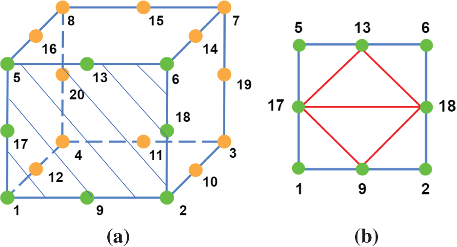
Figure 2: (a) Schematic of 20-node hexahedral element, (b) Schematic of the front quadrilateral face subdivided into six triangular faces. Front surface of 3D element corresponding to measurement surface is cross-hatched and shown in (b)
The converted triangular mesh is subsequently written as a VTK PolyData surface and stored in VTP file format. Since external Python libraries, such as the VTK library, are not accessible within the scripting interface of ANSYS or ABAQUS, the VTP files are manually written in the appropriate XML syntax. To process the measurement data, the *. OUT file from VIC-3D [18] is interpreted using VicPy.
2.3.1 Transformation of Model Positions and Output into Measurement System
Once the rigid body transformation from model system to measurement system is determined through common feature identification in both the model and physical specimen, and both measurement and field data are available, model nodal coordinates and model output variables are transformed into the reference measurement coordinate system. Consistent with continuum concepts [19], the transformation of model variables into the measurement coordinate system using the optimally determined rotation matrix, [R], and translation vector, {t}, can be written in index notation as follows:
where Rij denotes components of the orthonormal rotation matrix transforming the model system into the measurement system, ti are components of the translation of model system origin to the measurement system origin, ‘exp’ denotes the transformed model data in the reference experimental measurement system, ‘mod’ denotes values in the model coordinate system, ui denotes three components of the displacement vector, and εij denotes components of the strain tensor. In Eqs. (1b)–(3), the summation convention on repeated indices is used. Since Eq. (2) is applicable to any vector output variable (e.g., velocity and acceleration) and Eq. (3) is applicable to similar 2nd order tensor quantities (e.g., gradients of displacement, ∂ui/∂xj), the same algorithms can be used for any vector or 2nd order tensor quantity defined in the model coordinate system.
2.3.2 Interpolation of Model Data to Measurement Locations
Once the two coordinate systems have been aligned and the model data (nodal positions, all model output variables) are transformed into the measurement coordinate system, an additional Python script is executed to (a) assemble each node of the triangulated finite element mesh into a K-D tree, (b) loop over each point in the DIC dataset and query the K-D tree to identify at least six nodes within the finite element mesh that are closest to the current DIC point, (c) identify each triangular element connected to those nodes, (d) project the measurement location into each connected element, (e) determine which triangle the point falls within and (f) interpolate the model’s triangular mesh with barycentric coordinates using the procedure given in Appendix A to obtain field data at the same location as the DIC measurements. Using this process for interpolation, finite element data is accessible at every spatial location in the DIC dataset where the two data sets overlap.
To validate the concepts described above, experiments were performed multiple times with essentially identical results; the average results at each point are reported in this study. The material, specimen geometries, loading process, details for the non-contacting stereovision system, StereoDIC parameters, along with a flowchart for the process employed to convert stereovision images into full field displacements and strains, are given in this section.
All specimens were extracted from a 4.76 mm thick, hot rolled Al6061-T6 aluminum sheet, with the rolling direction aligned with the tensile loading direction. The geometry for both the dog-bone tension specimens and the double edge-notched (DEN) specimens are shown in Figs. 3a and 3b, respectively. Each edge notch is machined as a semi-circular cutout with 20 mm diameter and a center-to-center distance between cutouts of 40 mm. Machining of the specimens was performed with a tolerance of 0.0254 mm. The mean dimensions are used in all simulations.
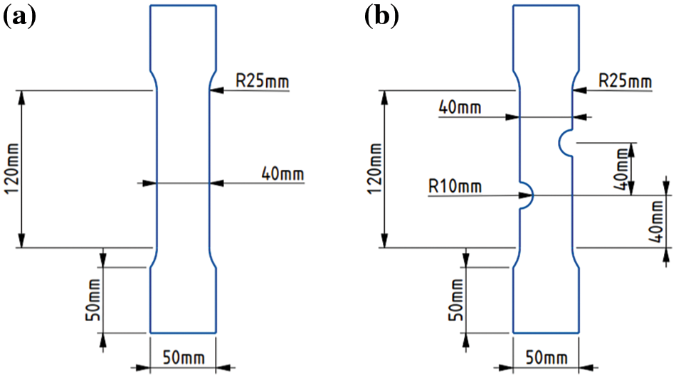
Figure 3: (a) Geometry of tensile specimen; (b) Geometry of double edge-notched specimen. All specimen thicknesses are 4.76 mm
To obtain uniaxial stress-strain data, two Al6061-T6 tensile specimens with geometries shown in Fig. 3a are subjected to tensile loading in an electromechanical MTS 810 test frame that has a maximum loading capacity of 250 kN. Clamp grips are used at the top and bottom to distribute the load more evenly across the specimen width. Average strain data is obtained using (a) a center-mounted strain gage rosette and (b) an MTS extensometer with a gage length of 25.4 mm attached to the gage section. Fig. 4 shows the average true stress-average true strain data for the material, with engineering axial strain, εaxial, converted to true strain, εtrue, using εtrue = ln (1 + εaxial) and engineering stress, σengr converted to true stress, σtrue, using the following formula σtrue = σengr (1 + εaxial). As shown in Fig. 4, Al6061-T6 is approximately bi-linear with a Young’s modulus, E = 71 GPa and a 0.2% offset yield stress of 290 MPa. Poisson’s ratio obtained from the strain gage rosette is ν = 0.34.

Figure 4: Average uniaxial true stress-true strain data for Al6061-T6
3.3 Mechanical Loading of Specimens
Like the loading process described for tensile specimens, each DEN specimen is loaded in tension via displacement control in the electromechanical MTS 810 load frame using clamp grips. A photograph of the test configuration, including a vertically oriented stereovision system to maximize image resolution along the specimen length, is shown in Fig. 5. All full-field displacement and strain data were obtained using stereovision with StereoDIC analysis of the images using VIC-3D software [18]. Details regarding specimen preparation for imaging, stereovision imaging, and StereoDIC analysis of the images are given in the following sub-sections.

Figure 5: Experimental test setup including (a) low heat LED light, (b) stereovision system with cameras on rigid bar rotated 90° to optimize spatial resolution along length, (c) DEN specimen with speckle pattern, (d) hydraulic clamp grips, (e) MTS 810 electromechanical test frame and (f) tripod with attachment or rigid bar with camera mounts. Large Inset: DEN specimen with speckle pattern. Small Inset: Close-up of speckle pattern on specimen
To place a high contrast speckle pattern on the specimen surface, the specimen surface is slightly roughened, cleaned with alcohol, and lightly coated with flat white paint. The speckle pattern is applied using black ink and a patterned rubber roller [20] with an average speckle size of 0.33 mm. Fig. 5 shows the specimen after speckle pattern application, along with a close-up image of the speckle pattern.
3.5 StereoDIC Principles for Full-Field Deformation Measurements
Since all full-field deformation measurements were obtained using stereo images and the non-contacting StereoDIC analysis method [21], the measurement method and how it is used to obtain measurements are described. Fig. 6 shows a schematic of two pinhole cameras that are used to model the imaging process for a stereovision system used with StereoDIC to measure the three-dimensional shape and deformation of a component. As shown in Fig. 6, a small region surrounding each spatial location, Q, is imaged by two cameras with pinhole locations P1 and P2, respectively. By applying a random pattern to the specimen, matching of the local patterns recorded by camera 1 and camera 2 requires an optimal search process in the sensor plane to obtain the pixel coordinates of Q in the camera 1 and camera 2 sensor planes. To convert the optimally matched sensor locations in camera 1 and camera 2 into the three-dimensional coordinates of Q, the pinhole model parameters for each camera must be determined as accurately as possible. Typical parameters for a pinhole camera model are (a) the focal length, f, (b) the location in pixels of the sensor plane center, (Cx, Cy), (c) the scale factor, λ, converting sensor coordinates into metric units (not shown in Fig. 6), (d) translation vector between global system and each pinhole, (e) orientation of each camera coordinate system relative to the global system which has three independent angles (not shown in Fig. 6) and (f) correction factors to account for deviations of the actual camera imaging process from the assumed pinhole model. A common image correction is for radial distortion due to deviation of the lens geometry from an ideal spherical lens shape. In this work, the correction terms are κ1 r3 and κ2 r5, where r is measured from the sensor plane center located at (Cx, Cy).

Figure 6: Schematic of a two-camera stereovision system individually modeled as pinhole cameras with pinholes P1 and P2
Finally, once each camera’s position and orientation relative to the global system are known, the position of the camera 2 system relative to the camera 1 system (e.g., baseline vector shown in Fig. 6) with components (Tx, Ty, Tz), and the relative orientation of camera 2 with respect to the camera 1 system are calculated, which again has three independent angles (α, β, γ). To obtain the required camera parameters, a calibration process is performed as discussed in the following section.
3.6 Camera Calibration Procedure and Parameter Estimates
To perform camera calibration, the authors acquired synchronized stereo images of a 14 × 10 array of 10 mm white dots on a rigid black calibration target for a range of three-dimensional rotations and translations. In this study, 35 image pairs of rotated and translated target images are acquired and a bundle adjustment procedure using VIC-3D Versions 9 and 10 (with Iris) software [18] is used to perform the optimal camera parameter estimation process. The resulting calibration parameters for both cameras are given in Table 1, including parameters for the transformation from camera 1 to camera 2 pinhole coordinate system.
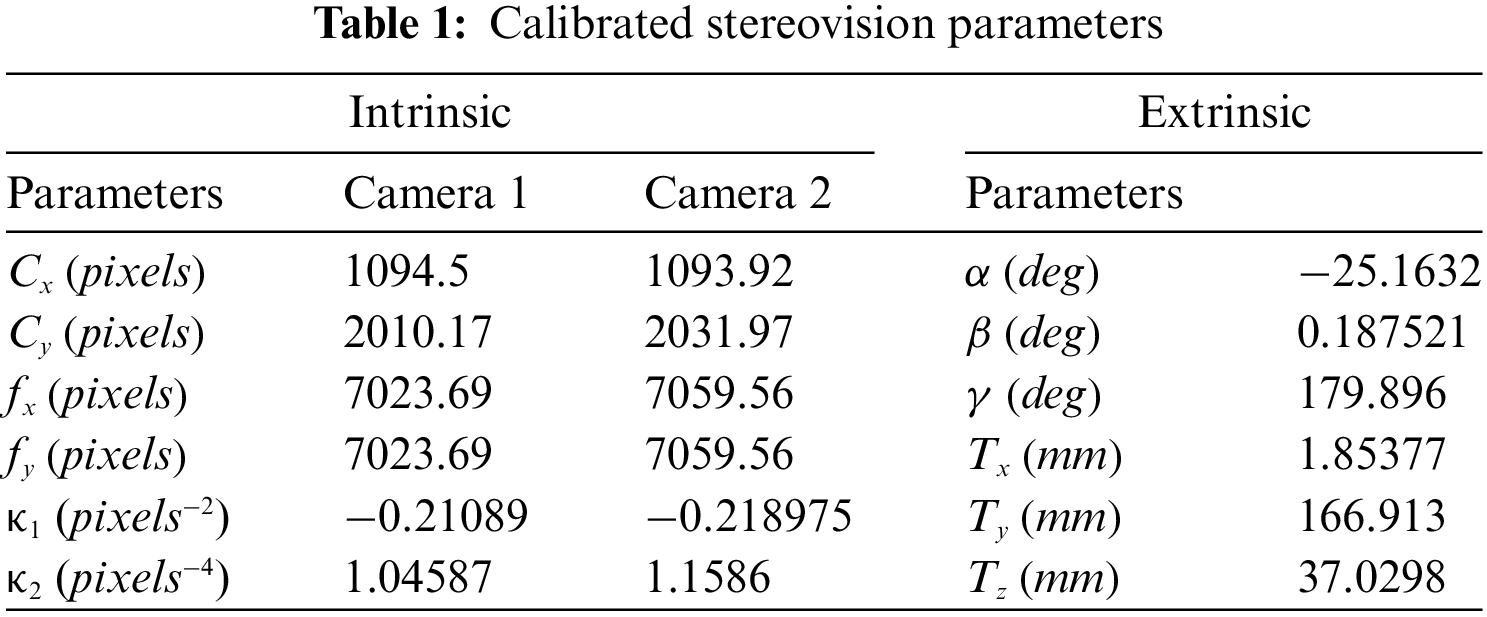
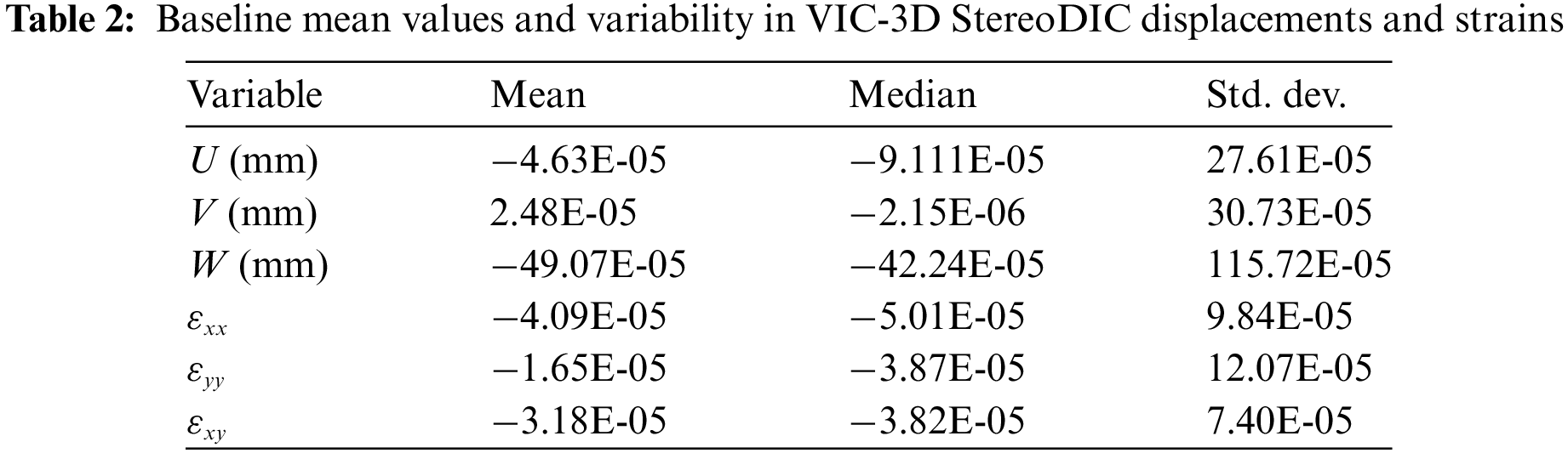
Fig. 7 presents an overview of the process used to convert synchronized stereovision images into full-field surface positions, displacements, and strains. To obtain baseline estimates for variability in strain and displacement measurements, the procedure outlined in Fig. 7 is used to compare four pairs of synchronized stereo images that were obtained prior to mechanical loading. Table 2 shows the measured variability and mean values for the displacements and strains when using a 45 × 45 subset and a 5-pixel subset spacing. As shown in Table 2, the mean strains are near zero with all standard deviations less than 125 µε throughout the entire specimen.1

Figure 7: Overview of the main steps to obtain 3D surface position, displacement and strain field measurements using stereo images and StereoDIC with VIC-3D for image analysis
3.7 Stereovision System and Image Acquisition for Experimental Measurements
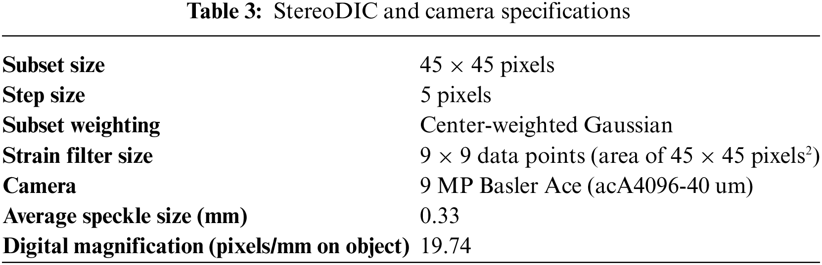
StereoDIC image analysis parameters and details for the Basler Ace cameras used in the experiments to obtain measurements from the speckle pattern images shown in Fig. 6 are given in Table 3. As shown in Table 3, each speckle is imaged by a 6 × 6 pixel2 area, which is more than the minimum required for accurate StereoDIC displacement and strain measurements [21]. During the loading process, synchronized stereo image pairs are acquired every 0.5 s using VIC-Snap software [22] as the specimen is subjected to a displacement rate of 0.06 mm/s. Testing continued until the initial cracking of the tensile specimen was observed. In this study, a total of 40 image pairs obtained during the first 20 s of testing were used to obtain full-field displacements and strains.
3.8 Measured Surface Strain Fields
For the 170 mm by 40 mm surface area on the DEN specimen shown in Fig. 5, over 100,000 deformation measurements are obtained using StereoDIC software VIC-3D, with a spacing of 0.25 mm between each data point. Due to the density of the measurements, most of the results are shown as full-field plots. Fig. 8 presents the measured full-field total strains εxx, εyy and εxy on the DEN specimen surface for tensile loading P = 8.3 kN, 18.3 kN, 30.5 kN and 35.1 kN. As shown in Fig. 8, all strains are relatively small when P ≤ 18.3 kN, with indistinct strain variations around the notches. For P > 18.3 kN, variations in strain around the notch tips and between the two notches are clearly visible, with εyy reaching its maximum at the notch tips for P = 35.1 kN.

Figure 8: StereoDIC strain measurements for four tensile loads
For comparison to experimental measurements, all calculations are obtained using commercial software, ANSYS [23], with theoretical details for the isotropic von Mises yield criterion and Hill’s anisotropic quadratic yield (HAY) criterion given in the following sub-sections. In order to define the linear elastic material response range, input material properties include the modulus of elasticity, Poisson’s ratio, and yield stress obtained from the uniaxial experiments performed by the authors, as described in Section 3.2. For stress states beyond the yield stress, the effective stress (i.e., the applied stress for the uniaxial specimen) and the uniaxial plastic strain are input into ANSYS at several points along the measured stress-strain curve, with linear interpolation used within the software to define stress-strain states between data points.
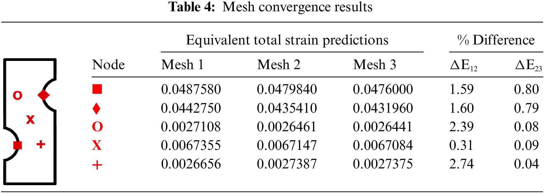
Fig. 9 shows the FE model for the DEN specimen. To ensure accuracy of model predictions, a mesh convergence study was conducted for three different structured hexahedral meshes labeled Mesh 1, Mesh 2 and Mesh 3 in Table 4 by applying the largest load, P = 35.1 kN. The meshes contained 102,503, 179,572 and 305,319 nodes and 19,980, 35,200 and 63,200 20-node quadratic (ANSYS SOLID186) elements, respectively. As shown in the graphic attached to Table 4, results are obtained at five nodes, including nodes at both notch tips. Defining the percent change in total strain, εT, as a function of mesh density by ΔE12 and ΔE23 for meshes 1, 2 and 3, we can write:

Figure 9: (a) FEA mesh with the imposed boundary conditions of U, V (green area) and U, V, W (yellow line) displacements on the top and bottom of the specimen, (b) specimen geometry and DIC area of interest (red) within the FEA model
with εT defined as the sum of the effective elastic strain and effective plastic strain as follows:
Results for ΔE12 and ΔE23 at five nodal locations are shown in Table 4. Since there is less than a 1% change in εT at all nodes for Meshes 2 and 3, in this study, Mesh 2 was used in all simulations.
4.2 FE Model and Boundary Conditions
Regarding boundary conditions at the top and bottom of the FE model shown in Fig. 9, personal experiences of the authors with clamping grips suggest that specimen boundary conditions in the grips are difficult to quantify; clamping pressure variations across the width, the potential for specimen slippage and slight in-plane rotation of the specimen during gripping is high and has been observed in previous experiments [24], none of which can be represented by idealized gripping conditions. As shown schematically in Fig. 9, to account for such effects the authors selected a slightly reduced specimen length so that StereoDIC measurements could be obtained at the top and bottom of the specimen and applied as FE boundary conditions. Specifically, the following are the displacements that were applied for all simulations:
• Measured (U, V, W) displacements along two horizontal yellow lines spanning the specimen width at the top and bottom of the specimen are applied in the (x, y, z) directions, respectively, for each applied load level.
• Measured (U, V) displacements on the front surface are applied to all nodes through the thickness on the top and bottom of the specimen for each applied load.
• Integration of σyy on the top and bottom surfaces was performed to confirm the axial load corresponded to the load cell measurement.
• W displacements are not applied to nodes on the back surface.
Since loads are recorded every 0.5 s in correspondence to the experimental image acquisition rate, the measured displacements along the yellow lines are used as boundary conditions for each load step. Large-deformation effects are enabled in the analysis, though this option is not required since loading was terminated when the first crack was observed, and the strains are not large.
In addition to the displacement boundary conditions at the top and bottom of the specimen, additional boundary conditions for the model include traction-free conditions on the front, back, sides and notch surfaces in regions away from grips.
4.3 Material Properties and Plastic Flow
Since hot rolling may affect the response of the aluminum specimen during mechanical loading, the authors used both isotropic and anisotropic yield criteria in the FE simulations. For applications where the material responds isotropically during mechanical loading, the von Mises yield criterion [15] is one of the most used yield criteria. The von Mises yield criterion is independent of the first stress invariant or the hydrostatic component of stress at a point. As such, it is applicable for the analysis of plastic deformation in ductile materials (e.g., metals) since the onset of yield for these materials does not depend on the hydrostatic component of the stress tensor.
For applications where anisotropy in material response is present (e.g., sheet metal forming), four of the commonly used anisotropic yield criteria are the original Hill’s quadratic yield criterion [17], a modified Hill criterion developed decades later [25], the criterion of Barlat et al. [26] and a criterion developed by Banabic et al. [27,28]. The original Hill criterion stands out due to its simplicity, user-friendliness and the fact that only four parameters are required to predict yielding behavior. Though the other criteria have advantages when predicting response under a variety of loading conditions, they require a larger number of experimentally determined parameters, which is both expensive and time-consuming for a wide range of loading conditions. An additional concern is the availability of computational platforms capable of using various criteria in simulations. Typically, the original quadratic Hill criterion is available for simulations in FE codes such as Abaqus and Ansys, while implementation of others may require substantial time and expense to independently develop, validate and then incorporate as user subroutines within an FE code. In this work, the von Mises yield criterion and original HAY criterion are used to model the response of the Al6061-T6 specimen.
4.3.1 Von Mises Isotropic Yield Criterion
The von Mises yield criterion is a rate-independent, multilinear plasticity model. In this study, the authors used an associated flow rule and an isotropic hardening rule [21]. The von Mises yield criterion in terms of the effective stress is defined as follows [14,15]:
where
where
4.3.2 Hill’s Quadratic Anisotropic Yield Criterion (HAY)
The HAY criterion [17,23] is a quadratic function of normal stress differences and shear stresses but is not a function of pressure. The form used in these simulations can be written as follows in a coordinate system aligned with the anisotropy coordinate system.
where the coefficients F, G, H, L, M, N in Eq. (8) are six parameters that each the ratio of the yield stress for each of the six stress components to the uniaxial yield stress obtained from the tension experiment, as shown in Eq. (9).
The stress ratios or directional yield stress ratios,
where σy is the uniaxial yield stress along the length of the specimen (corresponds to σyy stress component, with the response shown in Fig. 4). When the directional yield stress ratios are equal to 1, the HAY criterion reduces to the von Mises yield criterion in Eq. (6).
5 Comparison of Co-Registered FE Predictions and Experimental Measurements at Same Spatial Locations
Comparison of the FE predictions and experimental measurements using both the von Mises and anisotropic Hill’s yield criteria are presented in the following sub-sections, with results showing the importance of comparing measurements and predictions at the same spatial locations.
5.1 FE Strain Field Predictions Using Von Mises Yield Criterion and Comparison to Measurements
Fig. 10 presents the FE strain field predictions for axial loads of 8.3, 18.3, 30.5 and 35.1 kN. A visual comparison of the full-field experimental results in Fig. 8 to the predictions in Fig. 10 suggests there is very good agreement of measurements and predictions, especially in the high strain regions near the cutouts. Though visually consistent, and a form commonly used by investigators to indicate model agreement with experimental measurements, in fact, this type of visual comparison is not a pointwise quantitative indicator. To provide quantitative comparisons, one must analyze point-by-point comparisons of the measured and predicted quantities at the same spatial positions. In this regard, closer visual inspection of Figs. 8 and 10 indicates that there are strain differences as large as 0.006 in regions near the notch tips where the highest stresses and strains occur. These localized regions of higher differences suggest there is an underlying reason for higher strain differences as the tensile load increases.

Figure 10: FE results using von Mises yield criterion for four tensile loads
To clearly show the differences between FE and StereoDIC measurements at the same spatial positions everywhere in the specimen, the FE and StereoDIC measurements are co-registered using the procedures outlined in Section 2. Fig. 11 shows line plots of the difference between FE predictions and StereoDIC measurements for (a) εxx and (b) εyy at various load levels along a horizontal line at the centerline of the bottom notch that starts at node ■ shown in Table 4. As shown in Fig. 11, the strain differences between the FE predictions and StereoDIC measurements increase when the applied load exceeds 18 kN and plastic deformations increase in the high stress notch region. Since (a) the strains are relatively small throughout the experiment, (b) the speckle pattern has high contrast, (c) the cameras sufficiently oversample the pattern to ensure accurate matching and (d) camera calibration was performed successfully and with low variability throughout the DEN specimen with standard deviation for all in-plane strain components less than 125 με, the differences shown in Fig. 11 are not due to experimental measurement factors.

Figure 11: Strain differences, Δεij = εij exp – εij mod, at four load levels for (a) εxx and (b) εyy at common spatial locations along a horizontal line at the center line of the bottom notch using the von Mises yield criterion
Since the results in Fig. 11 indicate the FE predictions are higher than the StereoDIC measurements, one possibility is the convergent FE mesh with quadratic shape functions near the notch is capable of more effectively resolving the local strain gradients near the notch than the StereoDIC measurement system which uses subsets and a strain window that are both 5.76 mm2 and a linear shape function, resulting in a higher local average value for the predictions. However, this seems at odds with the fact that the model predictions and measurements are in excellent agreement until the material undergoes local plastic deformation. To assess the level of agreement between FE and measurements for all strains throughout the entire specimen, Fig. 12 shows the point-by-point differences between FE predictions and StereoDIC measurements throughout the specimen. Inspection of Figs. 11 and 12 confirms that the notch region has the largest strain differences at higher loads for both normal strains εxx and εyy.
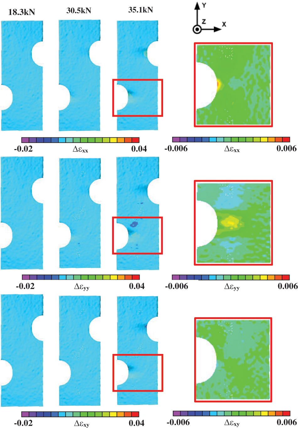
Figure 12: Full-field strain differences, Δεij = εij exp – εij mod, at common spatial locations throughout the region of interest using isotropic plasticity and hardening for three load levels. Here i, j = 1 is the x-direction and i, j = 2 corresponds to the y-direction
Though the strain differences shown in Figs. 11 and 12 are much smaller than the applied strain for each load level, it is equally clear that the largest differences occur in the high strain region near the notch tips where elastic-plastic material behavior is present. Since the Al6061-T6 material used in the experiments incurred manufacturing deformations during production that could result in anisotropic response (e.g., yield stresses in length, width and thickness directions may not be equal), the authors performed FE simulations of the DEN specimen using Hill’s anisotropic quadratic yield (HAY) criterion which requires estimates for the material parameters in the HAY criterion.
5.2 Parameter Determination and FE Strain Field Predictions Using HAY Criterion and Comparison to Measurements
As shown in Eqs. (8)–(10), the HAY criterion has six material parameters. Since measurements are obtained on the relatively thin, nominally planar, traction-free front surface of the DEN specimen that is being subjected to axial loading, the effects of σzz, σxz and σyz on the surface measurements are minimal and hence parameters L and M cannot be determined using only the surface measurements for the DEN specimen. However, for the nominally plane stress state on the front surface, there is sufficient variation in the x-y stresses and strains throughout the specimen (see Fig. 7) to optimally determine F, G, H and N parameters in Eqs. (8), (9), as detailed in the following subsections.
5.2.1 HAY Criterion Parameter Estimation
Since dense sets of full field strain measurements for εxx, εyy and εxy are obtained on the traction-free front surface of the DEN specimen at several load levels, the author used the measurements and known loads in an optimization process to quantify four HAY criterion parameters. To initiate the optimization process, the authors selected an initial set of HAY parameters based on the existing literature [29–31]. The authors then performed a gradient search process varying F, G, H and N in Eq. (8) in Hill’s anisotropic yield criterion, performing simulations to extract εxx, εyy and εxy predictions for point-by-point comparisons of FE predictions and experimental measurements.
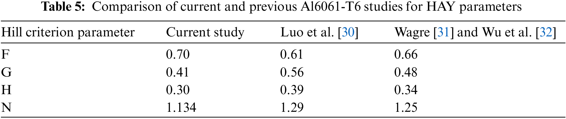
By varying one parameter at a time in the FE model and minimizing the difference between the FE strain predictions and the StereoDIC measurements throughout the specimen for 36 load levels2, the appropriate direction for future parameter increments is determined and the process continued until the % change in each parameter is less than 3%. The optimized computational predictions in terms of stress ratios are RS11 = 1.20, RS22 = 1.00, RS33 = 0.95 and RS12 = 1.15. Using these values in Eq. (9), the HAY parameters are F = 0.70, G = 0.41, H = 0.30 and N = 1.134.3
As to how well the HAY criterion parameters in this study compare to previous plane stress studies using Al6061-T6, Table 5 provides a comparison of our optimally estimated parameters to those obtained in previous studies [30–32].
5.2.2 FE Strain Field Predictions Using HAY Criterion and Comparison to Measurements
Fig. 13 shows the full-field strain predictions obtained using FE analysis with the HAY criterion and parameters shown in Table 1.4 Fig. 14 shows the difference between the predictions and experimental measurements in a small area just ahead of the lower notch tip. As shown in the higher magnification insets in Fig. 14, for all components of strain the maximum differences occur near the notch tips.

Figure 13: ANSYS full field finite results using the HAY criterion and isotropic work hardening

Figure 14: Full-field strain differences, Δεij = εij exp – εij mod, at common spatial locations throughout the region of interest using optimized anisotropy yield parameters and isotropic hardening for three load levels. Here i, j = 1 is the x-direction and i, j = 2 corresponds to the y-direction
To provide a direct comparison of FE predictions and StereoDIC measurements at a specific point, the authors selected a small region located just ahead of the notch tip (see the red region in Fig. 15), the StereoDIC measurements and FE predictions for the transverse strain, εxx, are averaged over the same area as the DIC subset size (2.28 mm × 2.28 mm). The difference between the spatially averaged experimental measurements and FE predictions, defined as Δεxx = εxx exp – εxx mod, is shown in Fig. 15 for all load levels. As was noted earlier, for low loads when the notch region remains elastic, there is virtually no difference between the FE predictions and StereoDIC measurements. However, for higher loads, as plasticity increases the strain differences are on the order of 300 µε, which is a twenty-fold reduction relative to comparisons using the von Mises yield criterion, clearly demonstrating the presence of anisotropy in material response.

Figure 15: Differences between computational prediction and experimental measurement of εxx at the same spatial position in region shown in red near notch tip as function of tension load for von Mises and Hill’s yield criteria
5.3 Comparison of Measurement-Based Stresses to Model Predictions
The point-by-point difference between model predictions and experimental measurements for strains shown in Fig. 14 was extended to stresses. To obtain full-field stresses from experimental StereoDIC strain measurements without employing FE modeling, the authors used the HAY criterion with the experimentally measured strains. To ensure that stresses obtained at the applied loads are accurate, the authors used (a) 36 full-field measurements of strain that corresponded to load increments of ~900 N or smaller and (b) a modified version of the incremental procedure for isotropic materials described previously [30] to obtain stresses after each load step using the HAY criterion. For applied loads of 18.5, 30.5 and 35.1 kN, Fig. 16 shows the point-by-point differences between StereoDIC measurements-based stresses and FE model predictions.

Figure 16: Full-field stress difference, given by Δσij = σij exp – σij mod, at same spatial locations throughout the region of interest using optimized anisotropic yield parameters and isotropic hardening for three load levels. Here i, j = 1 is the x-direction and i, j = 2 corresponds to the y-direction
As shown in Fig. 16, the FE stress predictions and the measurement-based stresses when using the HAY criterion are in excellent agreement throughout the domain, including the higher stress regions around the notches. Results show the maximum stress difference is ≤34 MPa throughout the domain, with these differences occurring in small, isolated regions away from the notch tips.
In the linear elastic regime, the StereoDIC strain measurements can be converted to stresses using the measured Young’s modulus, E, and Poisson’s ratio, ν. Using the measured strains and the elastic parameters, stresses at a notch tip can be determined and used to determine parameters such as the stress concentration factor, Kt, for the axial stress, σyy, and the associated notch sensitivity factor, q. Though Kt values for single edge notch specimens exist in the literature [33] and q values for similarly notched specimens [34], these estimates do not include the interaction of the notches in our DEN specimen. In this work, a direct comparison of notch tip Kt values obtained using FE simulations and StereoDIC measurement-based stresses is shown. Since σyyfar field = P/A and our far-field cross-sectional area is A = 190.4 × 10⁻⁶ m2, using the definition of Kt = σyynotch/σyyfar field, Fig. 17 shows both the FE and StereoDIC values for Kt at the bottom notch tip vs. σyyfar field. As shown in Fig. 17, there is very good agreement between the measurement-based Kt predictions which range from 4.3 to 5.0 with an average of ~4.6, and the FE predictions which range from 4.3 to 4.5 with an average of ~4.4.
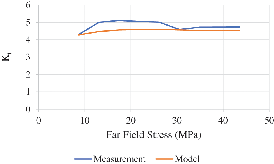
Figure 17: Kt vs. σyyfar field at the bottom notch tip using εyy measurements for stresses within the linear elastic range
Once Kt is determined, the notch sensitivity factor, q, can be estimated. Owolabi et al. [35] determined the fatigue factor for Al6061, with Kf ≈ 1.76. Using the definition for Kf = 1 + q (Kt – 1). Fig. 18 shows a direct comparison of q values obtained from FE predictions and StereoDIC measurements-based values for a range of σyyfar field stresses. Inspection of Fig. 18 again shows very good agreement between the FE and StereoDIC measurement-based values for q.

Figure 18: q vs. σyyfar field at the bottom notch tip using εyy measurements to obtain stresses within the linear elastic range
As noted in [21] and shown in detail by investigators [36], a distinct advantage of the stereovision method used in this work relative to single camera imaging (such as was used in [2,4,5,8–13]) is the direct measurement of both surface shape and all three displacement components. This is in contrast with single camera measurements, where the strains are affected by out-of-plane motions. The use of stereovision with StereoDIC allows investigators to image complex, non-planar components and obtain accurate deformation measurements, regardless of the geometry or specimen motions, as long as the specimen surface remains in focus. To further clarify this issue, inspection of Fig. 15 shows that StereoDIC strain components in front of the bottom notch are in excellent agreement with FE predictions using the HAY criterion. To provide a quantitative metric for the strain errors that occur if single camera imaging with 2D-DIC is used to obtain the deformations, based on formulae given in [36], if the camera is placed ½ m in front of the specimen and there is a 1/2 mm out of plane displacement of the object at a point, the normal strains errors are 1 × 10⁻³ at this point, which is nearly 50% of a typical yield strain in aluminum and much larger than the strain differences shown in Fig. 13. Since slight motions are inevitable experimentally, either due to Poisson effects, grip issues, or slight changes in loading resulting in bending or torsion of the specimen, single camera imaging should be used with caution.
Inspection of the strain differences in Fig. 14 when using the HAY criterion with an optimally selected set of model parameters shows that a set of 4 parameters5 can be determined that nearly eliminates Δεxx, substantially reduces Δεyy and continues to maintain a small Δεxy. These results are consistent with previous studies [8], though in this work all the HAY criterion parameters are obtained using subset-based image analysis with StereoDIC for measurements and ANSYS simulations with gradient-based optimization to minimize the difference between measurements and model predictions. Furthermore, as shown in the higher magnification inset in Fig. 14, the maximum differences occur near the notch tips and are on the order of 300 µε or smaller for all three strain components. In this regard, though Table 1 indicates reasonably good agreement with our parameter estimates and previous studies for nominally plane stress applications, the range of stress states in the DEN specimen is limited to tension dominated conditions. Further investigations, including additional experiments for a range of specimen orientations and loading conditions, would be needed to improve confidence in the predicted HAY criterion parameters while also providing data to determine parameters L and M associated with through-thickness shear stresses that are minimal in the DEN specimen.
Regarding the determination of stresses using full-field measurements, for those cases where nominally plane stress conditions are present, the results in Fig. 16 clearly show that surface StereoDIC measurements can be used with appropriate material characterization models to obtain full-field stresses without the necessity for FE modeling and validation. The only requirement when using StereoDIC measurements with non-linear constitutive property models is to ensure that load steps where data is obtained are sufficiently small so that stress increments are obtained accurately.
As shown in Figs. 17 and 18, the methodology developed in this study to obtain stresses using StereoDIC measurements allowed the investigators to obtain estimates for both Kt and q at the notch tip that are in very good agreement with FE predictions. These findings are somewhat different from those obtained in previous studies [13] that employed 2D-DIC, most likely because the DIC data did not agree with the FE predictions at the notch tip.
Finally, in contrast to previous studies that used single-point strain measurement methods, such as [4,6,7], the enclosed study provides a dense set of measurements to make it easier to identify regions with higher strains. Identifying such locations is particularly important when comparing measurements to FE model predictions.
7 Longer-Term Implications and Applicability for Non-Planar and Composite Applications
The demonstrated ability to obtain accurate, full-field deformation measurements and combine these measurements with existing constitutive models to estimate constitutive model parameters and obtain full-field stresses without requiring independent computational modeling has the potential to significantly impact future mechanics of materials studies. The capability can be readily combined with measured mechanical loads and prescribed boundary conditions (e.g., traction-free boundaries) to ensure that measurement-based calculation of stresses is consistent with known conditions. In addition, the approach can be extended to dynamic applications where displacements, strains, velocities, and accelerations can be obtained experimentally at discrete time increments.
Conversely, the capability can also be inverted by defining a new FE type structure that can be combined with prescribed boundary conditions and known mechanical loads to extract a full field of material properties for a pre-specified constitutive model. Combining the calculated material properties with measured strains, the entire stress field can be determined, as shown above. A form of this inverted process has recently been proposed and conclusively demonstrated for one-dimensional applications by Rajan-Kattil et al. [37].
Regarding broader applicability of the approach to more complex geometries, the method using stereovision and StereoDIC to acquire dense sets of experimental data can be used with FE simulations for many structural shapes, including non-planar shapes, provided there is a surface on the structure where stereo images can be obtained. If the material system is nominally isotropic and the material properties are known (e.g., many metallic components, polymeric specimens and ceramic systems), then for surfaces where the pressure is known (e.g., a free surface), the experimental strain measurements can be used to obtain the entire local surface stress field and then used to compare with FE model predictions on the same surface. Examples would be (a) curved or flat surfaces of an aluminum aerostructure, as originally demonstrated by Sutton et al. [38], (b) web and/or flange regions of an I-beam [39], (c) region around a bolt as the bolted joint is assembled and then again during mechanical loading of the as-bolted joint [40], (d) mortar joints during mechanical loading or environmental changes [41], (e) underwater structures with sufficient visibility to observe deformations [42,43].
Use of the method to obtain pointwise stresses from the StereoDIC measurements can be used for some anisotropic materials, specifically those where there is minimal coupling between the stresses on the surface and the through-thickness shear stresses/strains that cannot be readily measured. For example, if x and y are local tangent vectors at a point on a composite surface, then the strains εxx, εyy and εxy can be measured. These can be used with FE simulation predictions for the same strains to assess the level of agreement between FE strain predictions and measurements. However, if the measured surface strains are to be used to predict surface stress, then the surface stresses must not be coupled to strains such as εxz which cannot be measured on the x-y surface and would require additional measurements or independent experiments to quantify.
Finally, given the current interest in machine learning and artificial intelligence for a range of problems, the ability to obtain dense sets of material property measurements for a broad range of mechanical loading conditions and specimen geometries seems to be an ideal situation where data sets can be used for training. As an example, it has been shown on numerous occasions that a first-order effect of damage in a material is to reduce the local “stiffness” of the material, which would correspond to reductions in the elastic modulus. By subjecting a specific material to a range of mechanical loading conditions while measuring the local modulus at discrete load levels, the measured changes in modulus can be combined with independent measurements of local damage (e.g., visual observations for thin structures, CT scans for three-dimensional components), using the dense data sets to train an ML model to identify local damage through correlation with property changes.
Registration and field comparison procedures have been developed, implemented, and successfully validated to compare full-field measurements and FE predictions at the same spatial locations. To compare FE predictions to measurements at the same locations, the procedures include (a) conversion of FE surface discretization into a structured triangular mesh using Python extensions for ease in interpolation of field quantities at common spatial positions, (b) output of triangular mesh descriptors (nodes, connectivity, field data at nodes) in a VTP format, (c) conversion of the model coordinate system into the measurement coordinate system, and (d) development of Python script with FE predictions and measurement-based results for use with a K-D Tree search process to project measurement points onto model triangular mesh and identify the appropriate element location to perform interpolation using barycentric coordinates of all ANSYS field quantities at each common measurement-model spatial location.6
To demonstrate the approach, a DEN tensile specimen, designed and manufactured using Al 6061-T6, is subjected to far-field tensile loading at a displacement rate of 0.06 mm/s, with full-field deformation obtained by performing StereoDIC with VIC-3D using stereo images captured at 2 Hz using VIC-Snap image acquisition and synchronization software. For comparison to StereoDIC measurements, the specimen is modeled using ANSYS software. Using the field comparison processes developed by the authors, StereoDIC measurements and ANSYS model predictions are compared at the same spatial positions throughout the entire specimen. Strain predictions using an isotropic yield criterion indicate excellent agreement between FE and StereoDIC measurements in the early-to-mid stages of loading, with larger strain differences near the notches occurring as the specimen undergoes increasing plastic deformation in these areas during loading. Finite element predictions of strain and stress using Hill’s anisotropic yield criterion with optimally selected material parameters are in very good agreement with observations for all applied loads, though future studies should include an independent set of experiments to improve estimates for the anisotropic material parameters.
Acknowledgement: The support of Correlated Solutions Incorporated and the Department of Mechanical Engineering at the University of South Carolina is gratefully acknowledged.
Funding Statement: Financial support provided by Correlated Solutions Incorporated to perform StereoDIC experiments and the Department of Mechanical Engineering at the University of South Carolina for simulation studies is deeply appreciated.
Author Contributions: The authors confirm contribution to the paper as follows: concept development, writing, editing and overall management, Michael Sutton; experiments, data analysis, initial writing, extensive editing, simulations, Troy Myers; code development for StereoDIC and editing, Hubert Schreier; StereoDIC experiments and image acquisition, Alistair Tofts; data analysis, editing, experiment oversight and modification, Sreehari Rajan-Kattil. All authors reviewed the results and approved the final version of the manuscript.
Availability of Data and Materials: Images, which are the basis for all experimental measurements, are available upon request for re-analysis by interested individuals. In addition, as noted in Appendix B, the software to perform field comparisons of Ansys and VIC-3D data at the same spatial positions is available by request from Correlated Solutions Incorporated.
Conflicts of Interest: Investigators are either employees of Correlated Solutions Incorporated or the University of South Carolina. Since the work performed focused on developing and disseminating a methodology for comparison at the same spatial positions of both simulation predictions and full-field measurements, with the software for doing this available by request, the authors do not believe there is a conflict of interest.
1When a specimen surface is modified to include a random, high contrast pattern, optimal matching of the common specimen region imaged by both cameras is sufficient to ensure that surface shape can be measured without incurring “ill-posedness” in the process. The main requirements are (a) sufficient contrast in the random pattern to accurately match the patterns in the stereo image pair and (b) sufficient density of the random pattern to ensure that there are sufficient StereoDIC measurements in a region to elucidate important local shape changes.
2The parameters were varied iteratively to obtain the optimal set of parameters based on minimization of Δεij in the entire region of interest. During the optimization process, the data obtained for the four load levels shown in Figs. 10–12 and none of the data comparing FE and StereoDIC measurements are used in the optimization process.
3For our nominally plane stress cases, it is common practice to set RS13 and RS23 to either 0 or 1 since these stresses are zero on the front surface and cannot be determined using free surface strain data. In this study, the authors set RS13 = RS23 = 1.
4The 36 loads used to optimally determine parameters for the HAY criterion did not include the four in Fig. 13.
5The two parameters associated with σxz and σyz cannot be determined in this case since these stresses are zero on the free surface where data is being obtained. Typically, these two parameters are either set to zero or to unity, an indication that the loading is nominally a planar state in the x-y plane.
6Conversion and comparison software used in this study to compare FE output to measurements and measurement-based stresses are listed in Appendix B. The listed software is available from www.correlatedsolutions.com for general use.
References
1. Kobayashi AS. Hybrid experimental-numerical stress analysis. Exp Mech. 1983;23:338–47. doi:10.1007/BF02319261. [Google Scholar] [CrossRef]
2. McNeill SR, Sutton MA. A development for the use of measured displacements in boundary element modelling. Eng Anal. 1985;2(3):124–7. doi:10.1016/0264-682X(85)90015-2. [Google Scholar] [CrossRef]
3. Wei Z, Deng X, Sutton MA, Yan J, Cheng CS, Zavattieri P. Modeling of mixed-mode crack growth in ductile thin sheets under combined in-plane and out-of-plane loading. Eng Fract Mech. 2011;78(17):3082–101. doi:10.1016/j.engfracmech.2011.09.004. [Google Scholar] [CrossRef]
4. İplikçioğlu H, Akca K, Çehreli MC, Şahin S. Comparison of non-linear finite element stress analysis with in vitro strain gauge measurements on a Morse taper implant. Int J Oral Max Impl. 2003;18(2):258–65. [Google Scholar]
5. Ramos T, Braga DF, Eslami S, Tavares PJ, Moreira PM. Comparison between finite element method simulation, digital image correlation and strain gauges measurements in a 3-point bending flexural test. Procedia Eng. 2015;114:232–9. [Google Scholar]
6. Pany C. Cylindrical shell pressure vessel profile variation footprint in strain comparison of test data with numerical analysis. Liq Gas Energy Res. 2021;1(2):91–101. doi:10.21595/lger.2021.22163. [Google Scholar] [CrossRef]
7. Pany C. Estimation of correct long-seam mismatch using FEA to compare the measured strain in a non-destructive testing of a pressurant tank: a reverse problem. Int J Smart Veh Smart Transp (IJSVST). 2021;4(1):16–28. doi:10.4018/IJSVST.2021010102. [Google Scholar] [CrossRef]
8. Réthoré J, Leygue A, Coret M, Stainier L, Verron E. Computational measurements of stress fields from digital images. Int J Numer Meth Eng. 2018;113(12):1810–26. doi:10.1002/nme.5721. [Google Scholar] [CrossRef]
9. Musial S, Nowak M, Maj M. Stress field determination based on digital image correlation results. Arch Civ Mech Eng. 2019;19:1183–93. doi:10.1016/j.acme.2019.06.007. [Google Scholar] [CrossRef]
10. Lee J, Jeong S, Lee YJ, Sim SH. Stress estimation using digital image correlation with compensation of camera motion-induced error. Sens. 2019;19(24):5503. doi:10.3390/s19245503 [Google Scholar] [PubMed] [CrossRef]
11. Torabi AR, Bahrami B, Ayatollahi MR. On the use of digital image correlation method for determining the stress field at blunt V-notch neighborhood. Eng Fract Mech. 2020;223:106768. doi:10.1016/j.engfracmech.2019.106768. [Google Scholar] [CrossRef]
12. He J, Lei D, Cui X, Bai P, Zhu F. Characterization method of ITZ in concrete and measurement of nominal compressive elastic modulus based on SEM and DIC. Int Conf Comput Exp Eng Sci. 2019;21(4):78. doi:10.32604/icces.2019.05228. [Google Scholar] [CrossRef]
13. Romanowicz PJ, Szybiński B, Wygoda M. Application of DIC method in the analysis of stress concentration and plastic zone development problems. Materials. 2020;13(16):3460. doi:10.3390/ma13163460 [Google Scholar] [PubMed] [CrossRef]
14. Yasmeen F, Sutton MA, Deng X, Ryan M, Reynolds AP. Parameter estimation and application of anisotropic yield criteria for cylindrical aluminum extrusions: theoretical developments and StereoDIC measurements. Appl Sci. 2021;11(20):9701. doi:10.3390/app11209701. [Google Scholar] [CrossRef]
15. Von Mises R. Mechanics of solid bodies in the plastically-deformable state. Nachrichten von der Gesellschaft der Wissenschaften zu Göttingen, Mathematisch-Physikalische Klasse. Göttin Nachr Math Phys. 1913;1:582–92 (In German). [Google Scholar]
16. Barlat F, Lege DJ, Brem JC. A six-component yield function for anisotropic materials. Int J Plast. 1991;7(7):693–712. doi:10.1016/0749-6419(91)90052-Z. [Google Scholar] [CrossRef]
17. Hill R. A theory of the yielding and plastic flow of anisotropic metals. Proc R Soc London. Series A. Math Phys Sci. 1948;193(1033):281–97. doi:10.1098/rspa.1948.0045. [Google Scholar] [CrossRef]
18. VIC-3D software. Place Unknown: Correlated Solutions Incorporated. Available from: https://www.correlatedsolutions.com/VIC-3D. [Accessed 2023]. [Google Scholar]
19. Malvern LE. Introduction to the mechanics of a continuous medium. Englewood Cliffs, New Jersey: Prentice-Hall, Inc.; 1969. [Google Scholar]
20. Speckle kit. Columbia, SC: Correlated Solutions Incorporated. Available from: https://www.correlatedsolutions.com/accessories-ref/speckle-kits. [Accessed 2023]. [Google Scholar]
21. Sutton MA, Orteu JJ, Schreier H. Image correlation for shape, motion, and deformation measurements: basic concepts, theory and applications. 1st ed. New York: Springer Science and Business Media; 2009. doi:10.1007/978-0-387-78747-3. [Google Scholar] [CrossRef]
22. VICsnap software. Columbia, SC: Correlated Solutions Incorporated. Available from: https://www.correlatedsolutions.com/vicsnap. [Accessed 2023]. [Google Scholar]
23. ANSYS Inc. Theory reference. Release 2021 R2. Canonsburg, PA, USA: ANSYS Inc.; 2021. [Google Scholar]
24. Helm JD, Sutton MA, McNeill SR. Deformations in wide, center-notched, thin panels, part I: three-dimensional shape and deformation measurements by computer vision and part II: finite element analysis and comparison to experimental measurements. Opt Eng. 2003;42(5):1293–320. doi:10.1117/1.1566001. [Google Scholar] [CrossRef]
25. Hill R. Constitutive modelling of orthotropic plasticity in sheet metals. J Mech Phys Solids. 1990;38(3):405–17. doi:10.1016/0022-5096(90)90006-P. [Google Scholar] [CrossRef]
26. Barlat F, Lian K. Plastic behavior and stretchability of sheet metals. Part I: a yield function for orthotropic sheets under plane stress conditions. Int J Plast. 1989;5(1):51–66. doi:10.1016/0749-6419(89)90019-3. [Google Scholar] [CrossRef]
27. Banabic D. Yield criterion for orthotropic sheet metals. In: Proceedings of 8th International Conference on Metal Working-Metal Working 2000, 2000; p. 755–61. doi:10.1016/S0020-7403(03)00139-5. [Google Scholar] [CrossRef]
28. Banabic D, Kuwabara T, Balan T, Comsa DS. An anisotropic yield criterion for sheet metals. J Mater Process Tech. 2004;157:462–5. doi:10.1016/j.jmatprotec.2004.07.106. [Google Scholar] [CrossRef]
29. Sutton MA, Deng X, Liu J, Yang L. Determination of elastic-plastic stresses and strains from measured surface strain data. Exp Mech. 1996;36:99–112. doi:10.1007/BF02328705. [Google Scholar] [CrossRef]
30. Luo M, Wierzbicki T. Ductile fracture calibration and validation of anisotropic aluminum sheets. In: Proceedings of 2009 SEMAnnual Conference and Exposition on Experimental and Applied Mechanics, 2009; Albuquerque, NM, USA. p. 402–13. [Google Scholar]
31. Wagre D. Numerical analysis of forming of anisotropic sheet metals (Ph.D. Thesis). Universidade do Porto: Portugal; 2020. [Google Scholar]
32. Wu B, Ito K, Mori N, Oya T, Taylor T, Yanagimoto J. Constitutive equations based on non-associated flow rule for the analysis of forming of anisotropic sheet metals. Int J Precis Eng Manuf-Green Technol. 2020;7:465–80. doi:10.1007/s40684-019-00032-5. [Google Scholar] [CrossRef]
33. Baratta FI, Neal DM. Stress-concentration factors in u-shaped and semi-elliptical edge notches. J Strain Anal. 1970;5(2):121–7. [Google Scholar]
34. Zehsaz M, Hassanifard S, Esmaeili F. Fatigue life estimation for different notched specimens based on the volumetric approach. In: Proceedings of ICEM 14 14th International Conference on Experimental Mechanics for the EPJ Web of Conferences, 2010 Jul 4–9; Poitier, France. doi:10.1051/epjconf/20100642001. [Google Scholar] [CrossRef]
35. Owolabi G, Okeyoyin O, Bamiduro O, Olasumboye A, Whitworth H. The effects of notch size and material microstructure on the notch sensitivity factor for notched components. Eng Fract Mech. 2015;145:181–96. doi:10.1016/j.engfracmech.2015.03.026. [Google Scholar] [CrossRef]
36. Sutton MA, Yan JH, Tiwari V, Schreier HW, Orteu JJ. The effect of out-of-plane motion on 2D and 3D digital image correlation measurements. Opt Laser Eng. 2008;46(10):746–57. doi:10.1016/j.optlaseng.2008.05.005. [Google Scholar] [CrossRef]
37. Rajan-Kattil S, Sutton MA, Sockalingam S, Thomas F, Weerasooriya T, Alexander S. Direct material property determination: one-dimensional formulation utilising full-field deformation measurements. Strain. 2022;58(6):e12427. doi:10.1111/str.12427. [Google Scholar] [CrossRef]
38. Sutton MA, Matta F, Rizos D, Ghorbani R, Rajan S, Mollenhauer DH, et al. Recent progress in digital image correlation: background and developments since the 2013 WM Murray lecture. Exp Mech. 2017;57:1–30. doi:10.1007/s11340-016-0233-3. [Google Scholar] [CrossRef]
39. Xie X, Grace N, Kasabasic M, Patel K, Fong-Ramirez C, Ababio E. An application of digital image correlation (DIC) method in large-scale I-beams bending test. In: Proceedings of WCX World Congress Experience, 2018 Apr 16–18; Detroit, Michigan. p. 1–8. doi:10.4271/2018-01-1218. [Google Scholar] [CrossRef]
40. Mehrabian M, Boukhili R. 3D-DIC strain field measurements in bolted and hybrid bolted-bonded joints of woven carbon-epoxy composites. Compos Part B: Eng. 2021;218:108875. doi:10.1016/j.compositesb.2021.108875. [Google Scholar] [CrossRef]
41. Dzaye ED, Tsangouri E, Spiessens K, de Schutter G, Aggelis DG. Digital image correlation (DIC) on fresh cement mortar to quantify settlement and shrinkage. Arch Civ Mech Eng. 2019;19:205–14. doi:10.1016/j.acme.2018.10.003. [Google Scholar] [CrossRef]
42. Senol K, Shukla A. Underwater mechanical behavior of closed cell PVC foams under hydrostatic loading through 3D DIC technique. Polym Test. 2019;73:72–81. doi:10.1016/j.polymertesting.2018.11.003. [Google Scholar] [CrossRef]
43. Shukla A, Gupta S, Matos H, LeBlanc JM. Dynamic collapse of underwater metallic structures-recent investigations: contributions after the 2011 Murray Lecture. Exp Mech. 2018;58:387–405. doi:10.1007/s11340-017-0364-1. [Google Scholar] [CrossRef]
44. Vince J. Barycentric Coordinates. In: Mathematics for computer graphics. London: Springer-Verlag; 2006. p. 193–221. doi:10.1007/1-84628-283-7_11. [Google Scholar] [CrossRef]
45. Floater MS. Generalized barycentric coordinates and applications. Acta Numer. 2015;24:161–214. doi:10.1017/S0962492914000129. [Google Scholar] [CrossRef]
Interpolation Process Using Model Triangular Mesh
Using the procedure described in Section 2.3, Fig. A-1 shows schematically the triangle ∆ABC that contains the measurement point, P.
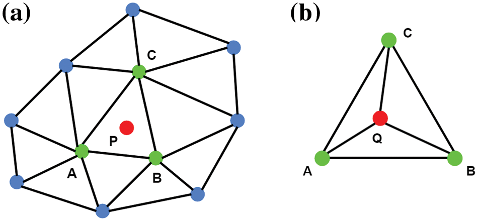
Figure A-1: (a) DIC point P (red) and the three closest finite element mesh nodes (green), along with the eight nodes in the connecting triangles; (b) Location, Q, of the perpendicular intersection (projection) of point P in ∆ABC
To obtain model field data at this point for comparison to the measurements, the measurement location, P, is projected onto ∆ABC using Eq. (A-1), where the interpolation process uses “barycentric” coordinates of the projected point, Q. To obtain the barycentric coordinates [44,45], the perpendicular projection of point P onto ∆ABC is required. The projection process is shown schematically in Fig. A-2, where d is the perpendicular distance from P to the intersection, Q. One set of equations that can be used to obtain the vector Q,knowing rA, rB, rC and rP in a common coordinate system, is given below.

Figure A-2: Graphical representation of process to obtain the intersection of the perpendicular projection of point P onto ∆ABC
First the normal to ∆ABC is given by the cross-product of two vectors in the plane.
where x denotes a cross-product. Since rA and rP have a common origin, the distance, d, to the plane from P is the normal component of the difference between the two vectors.
So that the three-dimensional location of the intersection, Q, can be written;
Once Qis determined, then the barycentric coordinates for interpolation can be obtained.
To obtain the barycentric coordinates, we define scalar parameters
with AABC = area of ΔABC, AQBC = area of ΔQBC and AQCA = area of ΔQCA. If the point is located inside the triangle, field variables such as strain are interpolated. For strain component εij, the value of strain at Q is interpolated using the values of strains at the corner nodes A, B, C as follows:
where:
Similar forms are used for vector components such as displacement and velocity.
Software for Conversion of Model Data to Measurement Coordinate System
Conversion and comparison software described in Sections 2.1–2.3.2 and used in this study to compare FE output to measurements and measurement-based stresses are available from www.correlatedsolutions.com for general use.
Available software includes:
• Python script to output ANSYS or ABAQUS data into a VTK PolyData surface and saved in a VTP file format.
• Software to transform all model information into the reference measurement system.
• Python script to assemble each node of the triangulated finite element mesh into a K-D tree and iteratively identify locations of measurement data within elements for interpolation of model data to common spatial location.
• Python script to compare measurements and model predictions at common spatial locations.
Cite This Article
 Copyright © 2024 The Author(s). Published by Tech Science Press.
This work is licensed under a Creative Commons Attribution 4.0 International License , which permits unrestricted use, distribution, and reproduction in any medium, provided the original work is properly cited.
 Downloads
 Citation Tools