Sensitivity Analysis of Electromagnetic Scattering from Dielectric Targets with Polynomial Chaos Expansion and Method of Moments

1  Introduction

Electromagnetic scattering simulation of dielectric conductors has become an essential tool in remote sensing, radar detection, and target stealth design. Currently, the primary numerical methods for electromagnetic scattering include the finite-difference time-domain (FDTD) method, finite element method (FEM), and the method of moments (MoM). The FDTD analysis method [1] replaces the curl equation in Maxwell’s equations in the time domain with finite differences, enabling the computation of field components. It is commonly employed in electromagnetics (EM) packaging, waveguide problems, and the study of wave propagation in complex (typically composite) materials. While it offers a straightforward mesh structure, it requires significant system memory and suffers from dispersion issues. Additionally, it encounters difficulties when handling irregular boundaries such as curved boundaries and thin media. On the other hand, the FEM is a variational technique used to solve boundary value electromagnetic problems in the frequency domain [2–4]. It is well-suited for solving problems with complex boundary shapes or conditions and involving complex media. FEM is commonly employed in the frequency domain to compute field distributions in closed regions like cavities and waveguides [5,6]. However, similar to FDTD, FEM needs the discretization and truncation of the solution domain, making it generally unsuitable for radiation or scattering problems unless integrated with boundary integral equation methods such as the MoM [7].

The MoM distinguishes itself from FDTD and FEM in that it specifically focuses on discretizing the surface or volume of the antenna or scatterer, as the electromagnetic source, whether it be surface or volume current, is the primary quantity of interest. As a result, MoM has gained wide usage in solving radiation and scattering problems, spanning across various fields such as dynamics [8], acoustics [9,10], magnetohydrodynamics [11], shape optimization [12,13], topology optimization [14–17], noise pollution treatment [18], and electromagnetic scattering analysis [19]. MoM is a technique that operates in the frequency domain, enabling the solution of electromagnetic surface or volume integral equations. This includes the utilization of coupled volume-surface integral equation (VSIE) solvers [20] and various surface integral equation (SIE) solvers. When dealing with uniform or piecewise uniform permittivity of the dielectric, SIE solvers are generally preferred due to their requirement of only surface discretization [21]. The present study focuses on employing the method of moments to solve electric field integral equations (EFIE) for radiation and scattering phenomena.

It is worth noting that although the MoM can achieve the desired accuracy, it entails solving a large matrix equation consisting of full elements [22]. This process demands significant storage and computational resources, even with high-speed and large-capacity computers. Consequently, the computational burden is substantial. To alleviate this challenge, several techniques have been employed to accelerate matrix computations, such as the SOAR method [23–27], generalized n-order perturbation method [28], fast multilevel method (FMM) [29,30], and surrogate model method [31,32]. However, the SOAR method usually discards some details and features in the original system which makes the reduced-order model unable to describe the behavior of the original system completely accurately and unable to effectively deal with systems with strong nonlinear properties; For the same problem, different parameter selection may lead to completely different results by the generalized n-order perturbation method. The FMM based on the MoM is an efficient algorithm and suitable for solving large-scale problems. However, the treatment of near-field effects and parameter selection require attention, and the complexity of the algorithm itself requires a certain amount of expertise and experience. The surrogate model approach can reduce the complexity of the problem by abstracting the original complex system into a simple model. Using a surrogate model can result in a dramatic increase in computation speed compared to the original system, especially if multiple iterations or optimizations are required. In addition, it is a non-embedded method and has stronger applicability, which makes the analysis and solution of problems easier and more efficient. So we adopt the surrogate model method in this work to establish a universal framework for reducing the calculation time of electromagnetic scattering problems.

In recent years, extensive research has been conducted by both domestic and international scholars to address the challenges of using surrogate models to reduce computational costs, improve optimization efficiency, and improve approximation accuracy. Commonly employed surrogate models encompass Polynomial Regression, Artificial Neural Networks (ANN) [33], Multivariate Adaptive Regression Splines [34], Radial Basis Functions (RBF) [35,36], Support Vector Machine (SVM) [37], Polynomial Chaos Expansion (PCE), and Kriging/Gaussian Process (GP) [38]. Among these, the PCE method offers significant advantages, including high accuracy in constructing surrogate models, and the efficient computation of system responses. In addition, the method can get an explicit expression, which is easy to understand and operate.

The PCE was initially introduced by Wiener [39], who employed Hermite polynomials to characterize stochastic processes involving Gaussian random variables. Cameron et al. [40] subsequently established the L2 convergence of PCE for any random process with finite second moments. Ghanem et al. [41] further combined this method with the finite element method to develop the Spectral Method for dynamic systems driven by random processes, yielding promising outcomes. Sensitivity is a crucial indicator for data analysis. It is important for a surrogate model to not only represent the information of the original model but also exhibit sensitivity information as much as possible. However, within the field of electromagnetic fields, there have been limited reports regarding the construction of surrogate models that utilize the PCE method for sensitivity calculations of electromagnetic scattering from dielectric targets.

It is worth noting that in the process of determining coefficients, selecting an improper order can lead to overfitting or underfitting phenomena, which significantly impact the accuracy of the PCE method. Consequently, this paper aims to bridge the gap between the surrogate model and sensitivity analysis and explicitly express the sensitivity of the EM scattering problem by employing an adaptive PCE algorithm to construct a surrogate model of EM scattering with appropriate orders. In summary, the key novelties of this paper are as follows:

1.   The adaptive PCE method based on the method of moments is proposed for electromagnetic scattering analysis of homogeneous dielectric (DIE) targets.

2.   This work presents the first sensitivity analysis method for electromagnetics with multivariate surrogate model.

The remainder of this paper is structured as follows. Section 2 presents the MoM for solving 2D electromagnetic scattering problems. Section 3 introduces the PCE method including the adaptive computing process and the evaluation criterion of the surrogate model. Section 4 provides various numerical examples to validate the proposed sensitivity analysis method. Conclusions are given in Section 5.

2  Electromagnetic Scattering Analysis by MoM

In this section, the MoM is applied to discretize the dielectric EFIE and obtain the surface current. The electric field radiation equations are subsequently coming into service for the scattering field, and the two-dimensional bistatic radar cross section (RCS) is eventually presented.

2.1 Electric Field Integral Equation (EFIE)

Considering a homogeneous dielectric body in the infinite domain, the simplified 2D schematic of electromagnetic scattering analysis is depicted in Fig. 1. ες denotes the permittivity of Ως.

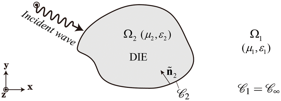
Figure 1: A homogeneous dielectric target residing within an infinite domain impinged by an electromagnetic plane wave: Ω1 is an unbounded domain in which the free space parameters are assigned (μ1,ε1), while the parameters are assigned (μ2,ε2) in the bounded-connected DIE region Ω2. The normal vector n~2 points into Ω2 from its interface. 𝒞2 denotes the boundary of Ω2

This bounded-connected DIE region Ω2 lies within the unbounded region Ω1. The permittivity and permeability are given by the scalars ες and μς, respectively, where the ς=1,2 represents the region. We further assume that a polarized time-harmonic electromagnetic plane wave with angular frequency ω and wave number k=ωεμ is implemented on the DIE. The EFIE on Ως can be expressed as

[jωμς(ℱJς)(ρ∗)+(𝒢Mς)(ρ∗)]tan+12n→ς×Mς(ρ∗)=[Eςinc(ρ∗)]tan(1)

where Eςinc(ρ) is the electric field generated by the incident wave and E2inc(ρ)=0. The operators ℱ and 𝒢 are

(ℱJς)(ρ∗)=[1+1k2∇∇⋅]∫G(ρ∗,ρ)Jς(ρ)d𝒞ς(ρ)(𝒢Mς)(ρ∗)=∇×∫G(ρ∗,ρ)Mς(ρ)d𝒞ς(ρ)(2)

where the G(ρ∗,ρ) denotes the Green’s function. For 2D problems, it is expressed as

G(ρ∗,ρ)=−j4H0(2)(kρ),withρ=|ρ∗−ρ|=(x−x∗)2+(y−y∗)2(3)

where H0(2)(kρ) denotes the Hankel functions of the second kind of order zero. ρ∗−ρ represents the vector from the source point to the field point, as shown in Fig. 2A.

Figure 2: Simple schematic of electromagnetic scattering problem: (A) The near field; (B) The bistatic angle θ; (C) The incident plane wave of TE and TM polarization

The above model can be simplified for computational convenience. Assuming the source point is the origin and the direction towards the field point is the positive x-axis, as shown in Fig. 2B, the angle through which the vector ρ∗−ρ rotates counterclockwise around the source point from the positive x-axis to the extension of the incident direction is called the bistatic angle, denoted by θ. The plane Sλ formed by the incident plane wave and the normal vector is defined as the incident plane. Based on the perpendicular or parallel orientation of the electric field component of the plane wave to the incident plane Sλ, it can be classified into transverse electric (TE) polarization and transverse magnetic (TM) polarization as shown in Fig. 2C.

It is obvious that the above integral equation is a variable coefficient, which is not easy to solve directly. To ensure the accuracy of the solution and the stability of the calculation process, the discretization method is used to transform it into a system of equations.

2.2 Discretisation of MoM

The MoM is used to convert Eq. (1) into a matrix system using Galerkin-type testing in each region. Expanding the electric and magnetic currents in Ως using a sum of weighted basis functions yields

Jς(ρ)=∑aςuς(ρ),Mς(ρ)=∑bςvς(ρ)(4)

where the triangle functions u1=−u2 and v1=−v2. The triangle functions w are applied to test the EFIE after discretization, which yields the matrix system in Ως as Eq. (5).

[AςBς][aςbς]T=Qς(5)

Aς(m,n) =jωμς[1+1k2∇∇⋅]∫wm(ρ∗)∫G(ρ∗,ρ)un(ρ)d𝒞ς(ρ)d𝒞ς(ρ∗)Bς(m,n) =∫wm(ρ∗)∫∇G(ρ∗,ρ)×vn(ρ)d𝒞ς(ρ)d𝒞ς(ρ∗) +12∫wm(ρ∗)⋅[n→ς(ρ∗)×vn(ρ∗)]d𝒞ς(ρ∗)Qς(m) =∫wm(ρ∗)⋅Eςinc(ρ∗)d𝒞ς(ρ∗)m,n=1,2,⋯Nς(6)

The matrices A and B respectively contain the quantities related to the virtual electric and magnetic current on the surface, and its dimensions are both Nς×Nς. The dimension of Qς is Nς×1. The sequences of a and b, both with dimensions of 1×Nς, can be expressed as aς=[a1a2⋯aNς],bς=[b1b2⋯bNς], respectively. The electric field integral equations over regions Ω1 and Ω2 are as follows:

[A1B1][a1b1]=Q1,[A2B2][a2b2]=Q2(7)

There are two unknowns in each EFIE in the two regions, which cannot be solved independently. Additionally, the tangential components of the electric and magnetic fields across the dielectric interface are by an amount equal to the magnetic and electric surface currents on that interface, respectively. The surface currents on dielectric interfaces are fictitious in Eq. (1). This implies that at the interface between Ω1 and Ω2, J1=−J2, M1=−M2. Therefore, the equations for the electromagnetic scattering system contain linearly dependent unknowns. This can be addressed by assigning an opposing orientation to the basis functions on opposite sides of an interface u1=−u2, v1=−v2, so that they will have the same coefficient, a1=a2,b1=b2, which is the unknowns that we want to solve [42].

Combining the equations above of the two regions Ω1 and Ω2, the system matrix over the entire domain is given by

[A 1B 1A 2B 2][ab]=[Q1Q2](8)

The coefficient a and b can be figured out by Eq. (8) and the electric and magnetic current can be further successfully obtained with Eq. (4).

2.3 Scattering Field

Here is the 2-D near-field radiation equations. The magnetic field radiated by an electric current is expressed as Eq. (9).

H(ρ)=jk4∫ 𝒞ς(ρ∗)(ρ∗−ρ)×J(ρ∗)H1(2)(kρ)ρd𝒞ςρ∗(9)

It can be rewritten by expanding into Cartesian components as Eq. (10).

Hscax(ρ) =jk4∫𝒞ς(ρ∗)([δyJz]H1(2)(kρ)ρ)d𝒞ς(ρ∗)Hscay(ρ) =jk4∫𝒞ς(ρ∗)([−δxJz]H1(2)(kρ)ρ)d𝒞ς(ρ∗)Hscaz(ρ) =k4∫𝒞ς(ρ∗)([δxJy−δyJx]H1(2)(kρ)ρ)d𝒞ς(ρ∗)(10)

where δx=x−x∗,δy=y−y∗. The corresponding electric field could be obtained by combining with Maxwell equation ∇×H=J+jωεE.

Escax(ρ) =k28ωε∫𝒞ς(ρ∗)(([δy2−δx2]Jx−2δxδyJy)H2(2)(kρ)ρ2−JxH0(2)(kρ))d𝒞ς(ρ∗)Escay(ρ) =k28ωε∫𝒞ς(ρ∗)(([δx2−δy2]Jy−2δxδyJx)H2(2)(kρ)ρ2−JyH0(2)(kρ))d𝒞ς(ρ∗)Escaz(ρ) =−k24ωε∫𝒞ς(ρ∗)(JzH0(2)(kρ))d𝒞ς(ρ∗)(11)

where H2(2)(kρ) denotes the Hankel functions of the second kind of order two. The Escax(ρ), Escay(ρ) and Escaz(ρ) above represent the 2-D scattering electric field in x, y and z directions, respectively. This is the penultimate step in solving the common response in electromagnetic scattering analysis.

2.4 Calculation of the Bistatic RCS for Electromagnetic Scattering

Sometimes people are interested in RCS, for which electromagnetics plays a critical important role. It is generally regarded as the equivalent scattering area of the object under a specific incident wave. It can be expressed as Eq. (12).

F2D=2πρ|Esca|2|Einc|2[m](12)

where ρ is the distance between the source point and the field point. The unit of RCS in Eq. (12) is m. Einc is already known by the incident electric waves, while Esca should be calculated with Eq. (11). The RCS is often expressed as Eq. (13) which is adopted in this work.

F2D=10×lg⁡F2D=10×lg⁡(2πρ|Esca|2|Einc|2)[dBm](13)

Generally speaking, the computational procedure for RCS is intricate, particularly when it involves computing a substantial full-element matrix. This complexity is further compounded by the extensive data computations required for uncertainty analysis, sensitivity analysis, and optimization. In light of these challenges, we propose the development of a surrogate model that can swiftly generate large-scale sample data.

3  Polynomial Chaos Expansion

PCE is a technique utilized to characterize the uncertainty inherent in random variables by formulating random spaces underpinned by polynomial bases. This method transforms the original nonlinear issue into a weighted sum of polynomials, essentially embodying a process of fitting coefficients. For any discrete data (u,y), it represents a function F∈𝒮 in a space spanned by multivariate polynomials Ai(u), with the infinite expansion

y=F(β,u)=β0A0(u)+β1A1(u)+⋯=∑i=0∞βiAi(u),i∈N(14)

where y is square-integrable and refers to the bistatic RCS in the electromagnetic scattering problem of this paper. βi denotes the unknown coefficients. The matrix Ai(u), composed by the multidimensional orthogonal polynomials, is related to the independent variable u, and u=(u[1],u[2],⋯,u[m]), where m refers to the dimension of the independent variable. For any single variable ui=(u1[i],u2[i],⋯,un[i]), the n represents the number of samples.

In practice, the above expansion should be truncated to contain a subset of polynomials, whose total degree does not exceed order o. Define the approximation space 𝒮o⊂𝒮 spanned by a set of finite-order orthonormal polynomials, the approximation Fo∈𝒮o is taken by Eq. (15).

y~=Fo(β,u)=β0A0(u)+β1A1(u)+⋯+βCAC(u)=∑i=0C−1Ai(u)βi,i∈NC⊂N(15)

where NC={0, 1, 2, …, C−1}, and C=(om+o)∈N. Ai(u)=[Ai(u1),Ai(u2),⋯,Ai(un)]. Subsequently, Eq. (15) can be simply rewritten as the following matrix form.

y~=Fo(β,u)=Aβ(16)

where

A=[A0(u1)A1(u1)⋯AC−1(u1)A0(u2)A1(u2)⋯AC−1(u2)⋮⋮⋱⋮A0(un)A1(un)⋯AC−1(un)]n×C(17)

and

β=[β0,β1,⋯,βC−1]TC×1(18)

where A is a matrix consisting of n rows and C columns, β is a matrix with C rows and one column, and (∼)T represents the transpose of the matrix ∼.

It is obvious that two primary factors must be taken into account in constructing the surrogate model with Eq. (16). The initial factor pertains to the construction of the orthogonal polynomial matrix A, while the second involves determining the coefficients represented by β. Subsequent sections will delve into these two critical aspects in detail.

3.1 The Construction of Orthogonal Polynomial Matrix

The dimensions of the independent variables differ greatly in the electromagnetic scattering system. For example, the bistatic angle θ can vary from a range of hundreds when measured in degrees, and the range of frequency f can be hundreds, thousands, or even millions. In order to reduce the influence of the magnitude of the independent variable on the fitting effect and improve the efficiency of the PCE method, the extreme value normalization method was applied firstly to obtain dimensionless independent variable u′, as shown in Fig. 3. In addition, the independent variables should be de-normalized to obtain the final surrogate model.

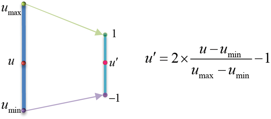
Figure 3: Normalization of independent variables u with the extreme value

The choice of one-dimensional orthogonal polynomials is often influenced by the distribution of the independent variables. For instance, Legendre polynomials are typically employed when the inputs exhibit a uniform distribution, whereas Hermite polynomials are favored for inputs that follow a Gaussian distribution. The standard recurrence relation for the Legendre polynomial system denoted as {Lk(u)}k=0o can be articulated as Eq. (19) within the interval [−1,1].

L0(u)=1,L1(u)=u,Lk+1(u)=2k+1k+1uLk(u)−kk+1Lk−1(u)1≤k≤o(19)

The formula for the general term of the Hermite polynomial system {Hk(u)}k=0o over the interval (−∞,∞) is presented in Eq. (20).

H0(u)=1,H1(u)=u,Hk+1(x)=uHk(u)−kHk−1(u)1≤k≤o(20)

Assuming m=1, the total count of orthogonal polynomial sequences is given by Eq. (21).

C=(o1+o)=(1+o)!1!⋅o!=o(21)

It can be easily obtained that the one-dimensional orthogonal polynomials Ai(u)=Li(u) or Hi(u), etc. In addition, these univariate polynomials are orthonormal concerning the probability density, i.e., ⟨Ai,Aj⟩=δij.

When m≥2, the multidimensional orthogonal polynomial matrix A(u) may be factorized into a series of one-dimensional orthogonal polynomials. The construction methodology for two orthogonal polynomials, up to the third order, is outlined in Table 1, exhibiting a structure reminiscent of Pascal’s triangle.

3.2 Calculation of the Unknown Coefficient

The truncated polynomial chaos expansion, as depicted in Eq. (15), represents a predicted value rather than an exact solution. Consequently, there exists an error between the predicted value and the true solution, which can be quantified as follows:

ε=y−y~=F(β,u)−F~(β,u)=∑i=C∞βiAi(u)(22)

where β represents the unknown coefficient vector. A smaller absolute value of the residual indicates a more accurate estimation of the surrogate model. The coefficient β should be chosen to minimize the expected value of the sum of squares of ε.

β^=arg⁡min1N∑(y−y~)2(23)

Thus, the PCE coefficient β^ can be determined by the following equation:

β^=(ATA)−1ATy(24)

The response from the surrogate model can be obtained with the solved coefficient β^ and Eq. (15). The measure commonly used to describe the accuracy of the final surrogate model obtained using the PCE method is the Root Mean Square Deviation Coefficient of Variation (RMSD-CV), abbreviated as CV in this paper, and expressed in Eq. (25).

CV(RMSD)=∑i=1n(yi−y~i)2n/∑i=1nyin(25)

where yi represents the output of the MoM, which serves as the input for PCE, and y^i represents the output of the obtained surrogate model using PCE. A lower value of CV indicates a better performance of the surrogate model. The numerator ∈R+ and the denominator ∈R. To facilitate the comparison of the accuracy of surrogate models of each order constructed with different original data, the absolute value of CV is used here. If the CV value is lower than 5%, it is considered that the expansion has converged at the current order and exhibits excellent fitting accuracy.

Based on the upper limit of CV that represents the accuracy of the surrogate model, the order can be iterated until CV <5%, at which point the design program can terminate to enhance the efficiency of constructing the surrogate model. The above PCE computational procedure is briefly described in Fig. 4.

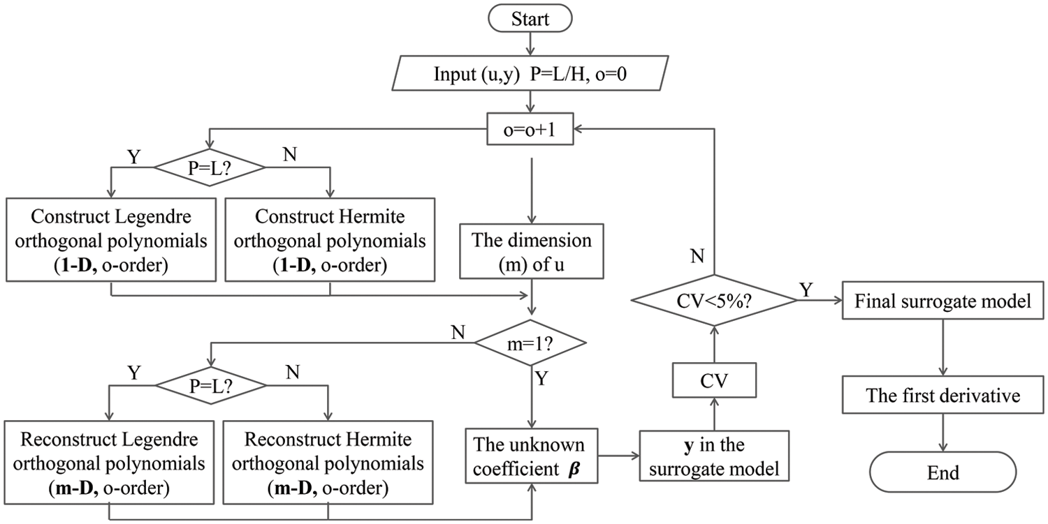
Figure 4: A brief flowchart for the calculation of the adaptive PCE method

The explicit expression of the surrogate model for the electromagnetic scattering problem can be derived using the MoM and PCE methods according to the above description. The model’s sensitivity concerning a specific variable can be obtained through differentiation, the calculation equations and precision of this method are described in detail in Section 4.3.

4  Numercial Examples

This section begins by using an example of a dielectric circular cylinder to validate the accuracy of the solutions obtained through solving the EFIE based on the MoM. Subsequently, the MoM solutions are utilized as input samples for the PCE method to construct univariate and bivariate surrogate models for electromagnetic scattering problems. The sensitivity results of each surrogate model are compared with those obtained from the finite difference method (FDM), followed by the verification of the PCE method for sensitivity analysis.

Both the dielectric cylinder and 5-bladed gear in this section are modeled by Non-Uniform Rational B-Splines (NURBS) in CAD. Both the basis function and the testing function in MoM are triangle functions, and the number of them are both 100 for interpolation calculation in CAE. The framework of the MoM is written in Fortran 90 language, and the adaptive PCE method is written using Matlab, which is run on a PC with an Intel (R) Core(TM) i7-7700 CPU and 128 GB RAM.

4.1 Scattering Verification with Cylinder Model

In this section, a dielectric cylinder model constructed using the control points (see Fig. 5) is applied to obtain the numerical solution of the two-dimensional electromagnetic scattering. The accuracy of the EFIE is demonstrated by comparison with the analytical solution (see Appendix A). Fig. 6 shows the RCS vs. frequency of the dielectric cylinder under TE-and TM-polarized incident waves, respectively. It can be seen that the results of EFIE are consistent with the analytical solution. In addition, with the increase of frequency, the bistatic RCS curves of this dielectric cylinder both exhibit significant fluctuations and are more drastic when θ=0 than θ=π in the same frequency band, which poses a challenge for the later construction of PCE surrogate model.

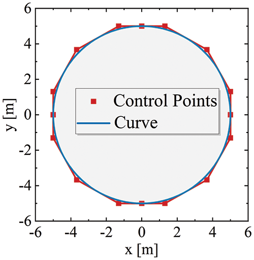
Figure 5: The sectional model boundary NURBS curve and control points

Figure 6: The bistatic RCS in terms of the frequency by numerical solution and the analytical solution with cylinder model, TE polarization, ε = 2. (A) θ=0; (B) θ=π

The following polar plots Fig. 7 describe the variation of bistatic RCS with θ under TE-and TM-polarized incident waves, respectively. The results of EFIE can also agree well with the results of the analytical solution in this case. It can be clearly seen that the curve is symmetric concerning θ=180∘, i.e., F(θ=m∘)=F(θ=n∘) at the same observation point if m+n=360.

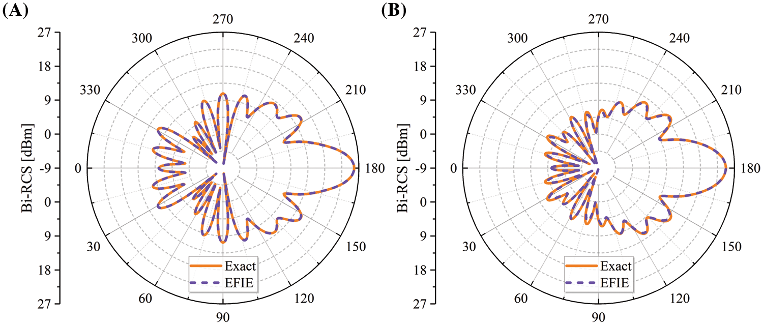
Figure 7: The bistatic RCS with respect to the bistatic angle θ=0 with cylinder model, ε = 2, f = 100 MHz. (A) TE polarization; (B) TM polarization

4.2 Scattering Problem with a 5-Bladed Gear Model

The dielectric 5-bladed gear model (see Fig. 8A) is analyzed for electromagnetic scattering using the EFIE method in this section. The dielectric 5-bladed gear has five uniformly shaped blades, which are modeled by the NURBS curve with 31 control points and further discretized into liner elements with a Dof of 100.

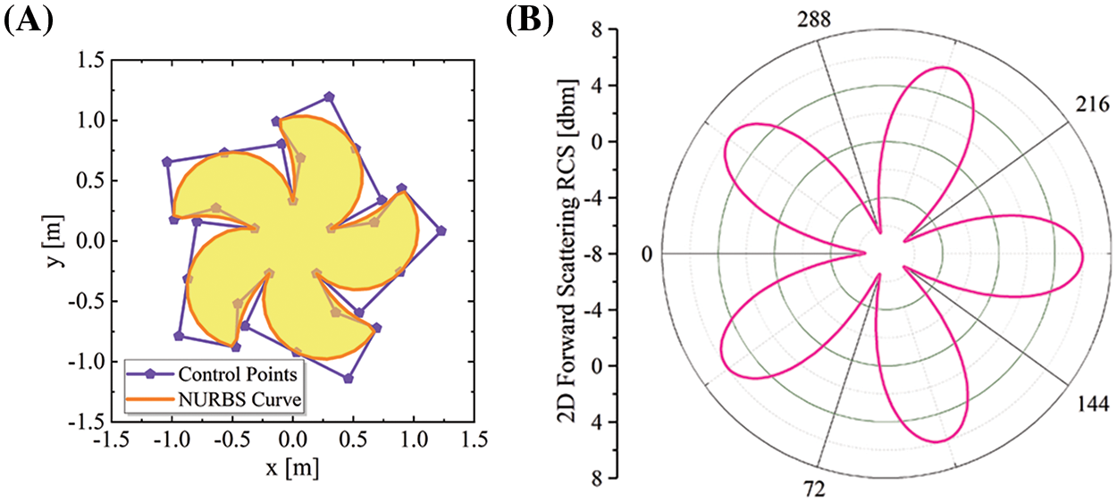
Figure 8: (A) The two-dimensional geometric model of the 5-bladed gear. (B) The forward scattering RCS in terms of the incident angle [ ∘] for 5-bladed gear: f = 100 MHz, ε = 5, TE polarization

The 5-bladed gear has 5-fold symmetry. Fig. 8B illustrates the forward scattering (θinc=θsca) RCS in terms of the incidence angle θinc, and the RCS cycles every 72 ∘ ( = 360 ∘/5), which fully demonstrates the 5-fold symmetry of it.

The bistatic RCS with a fixed observation point of the 5-bladed gear is not as symmetric as the cylinder model. The observation point is fixed at (1×105,0) m, Fig. 9 shows the bistatic RCS result of the 5-bladed gear model under TE-polarized incident plane wave, the results in (A) and (B) are no longer symmetric about a line, which is much different from the result in Fig. 7. It can be observed that F(θ=m∘)≠F(θ=n∘) at the same observation point if m+n=360, which can be seen more clearly in Figs. 9C and 9D. This is related to the fact that the 5-bladed gear is a rotation-symmetric model rather than an axisymmetric model. The distribution shape of the scattered field is different for the incident angle m∘ and n∘, and the scattered field at the observation point is not equal, resulting in different final bistatic RCS.

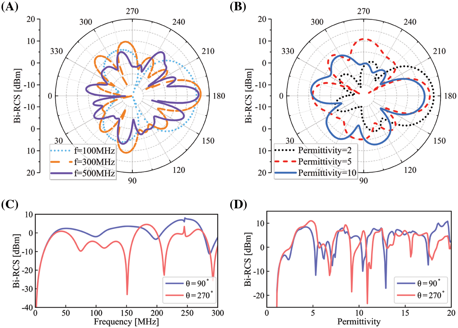
Figure 9: The bistatic RCS for 5-bladed gear model in terms of bistatic angle θ, frequency (f) and permittivity (ε) under TE-polarized incident waves

In addition, it can be seen that the bistatic RCS is related to the permittivity ε, the frequency f, and the bistatic angle θ. Any change in these values will result in a non-smooth change in RCS, therefore, it is necessary to implement sensitivity analysis, which can clarify the direction of optimization, reduce unnecessary calculation time, and improve optimization efficiency.

4.3 Sensitity Analysis with the Surrogate Model by PCE Method

In this section, the sensitivity analysis is performed with PCE and the global FDM. The objective function F is RCS, which denotes the response to the variable u=(u[1],u[2],u[3]). Here, u[1], u[2], u[3] represents the bistatic angle θ, the permittivity ε, and the frequency f, respectively. The sensitivity sequence of F(u) with FDM is defined by Eq. (26).

DFDM(ui+1+ui2)=Fi+1(u)−Fi(u)ui+1−ui(26)

The sensitivity sequence of bistatic RCS concerning the variable u with PCE is defined with the differentiation of explicit expressions of the surrogate model as Eq. (27).

DPCE(ui+1+ui2)=dFPCE(u)du|u=ui+1+ui2(27)

The sensitivity analysis of the homogeneous dielectric 5-bladed gear under TM-polarized incident plane wave is carried out here. The frequency f is set at 100 MHz and the permittivity is maintained at 2. Subsequently, the bistatic angle θ is varied from 0∘ to 180∘ in increments of 1∘. The 181 samples obtained by the MoM are divided into two parts, 38 samples are used as the training set (take the number at an interval of 5, plus the first and the end sample), and the remaining 145 samples are used as the test set. PCE method is used to construct surrogate models from order 2 to order 20 with the training set. The adaptive PCE program exits after the order reaches 15, while CV = 4.59%.

Fig. 10A visually shows the 38 training samples and the final surrogate model results, it is obvious that the 15th-order surrogate model can fit the training samples well. After that, the surrogate model results are compared with 145 test samples that are not involved in the training process, as shown in Fig. 10B, the surrogate model can predict the bistatic RCS of any points in the interval accurately.

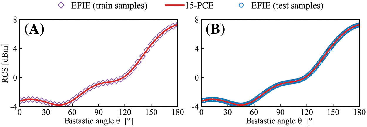
Figure 10: Comparison of training and testing results of the PCE method for 5-bladed gear model, f = 100 MHz, ε = 2, TM polarization

The sensitivity is obtained by taking the derivative of the explicit expression of the surrogate model, which is compared with the results of the FDM method. It can be seen from Fig. 11 that the surrogate model constructed by the PCE method can figure the sensitivity out accurately at any point in the interval only with a very small set of training samples, which is 38 points here.

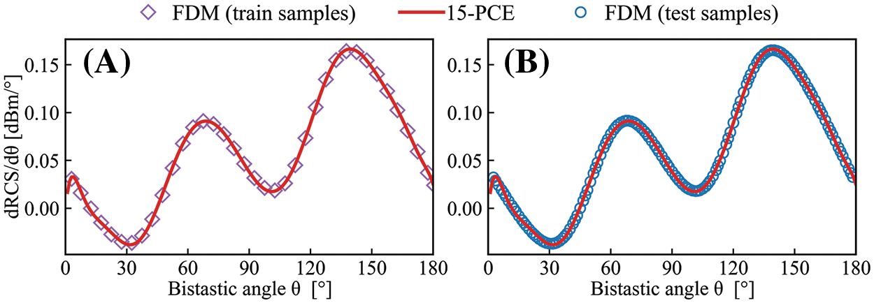
Figure 11: Sensitivity results D by FDM and PCE methods at training and test samples for 5-bladed gear model, f = 100 MHz, ε = 2, TM polarization

In addition, the sensitivity D is the largest while θ=141∘. Therefore, while f=100 MHz, ε = 2, the RCS is most sensitive to bistatic angle θ around 141 ∘.

As far as this surrogate model is concerned, the time needed to obtain a sample is about 0.455 s with MoM. The time required by combining the PCE method is mainly divided into three parts:

1.   Calculate 38 samples by MoM. This is a preparation for the next step and takes about 17.3 s.

2.   Construct surrogate model by PCE. The time required for the PCE method is little related to the number of sample points but mainly depends on the order of the surrogate model. In this example, a 15th-order surrogate model takes approximately 1.357 s.

3.   Solve the response. This process is based on the constructed surrogate model and requires about 2.04 s for 10,000 independent variables.

Fig. 12 shows the time required for the two methods to obtain samples in practice. The time required for MoM can be approximated as a linear function of sample size with a slope of 0.445. Since the PCE method requires a certain amount of initial samples as support, the MoM method should be used directly when calculating a sample size of less than 38. When 38 to 41 samples are needed, the combined method requires more computational time due to the process of constructing the surrogate model. The MoM should also be applied here. When the calculating size is more than 41, the time required by MoM continues to grow linearly, which barely grows by the combined method. It can be concluded that the combined method greatly improves the efficiency of electromagnetic scattering analysis.

Figure 12: The time required by the MoM and the combined PCE method

Fig. 13 shows the results of MoM and PCE methods of orders 5, 10, 15, and 20. Fig. 13A shows the results of each PCE method alongside the EFIE results. It is evident that the fitting accuracy is poor for the 5th-order PCE method; However, the curve of the PCE and MoM are visually consistent when the order reaches 10 and CV = 8.30%. The relative error corresponding to 5th, 10th, 15th, and 20th-order PCE method is presented in Fig. 13C. It is obvious that increasing the order will improve the accuracy of the surrogate model. In particular, the surrogate model with 20-order PCE largely reduces the fitting error on both sides of the interval. In addition, when the bistatic angle θ=118∘, the benefit of increasing the order on the fitting effect is little. This is because the point is located near the zero point of the original curve: F(θ=117)=−0.00231, F(θ=118)=0.07732, as shown in Fig. 13A.

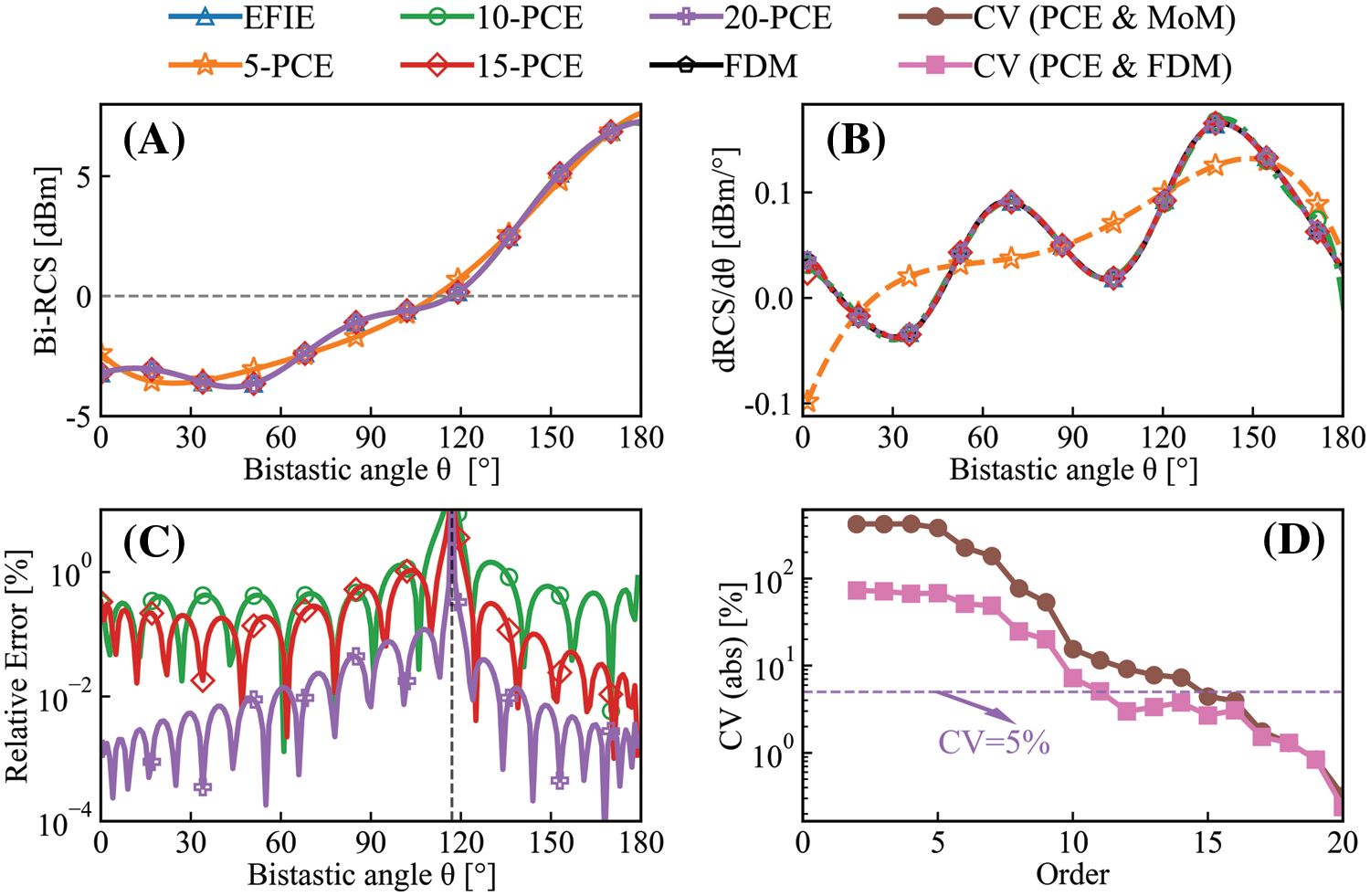
Figure 13: The PCE and sensitivity results at different order of the surrogate model by PCE for the 5-bladed gear model, f = 100 MHz, ε = 2, TM polarization

The “FDM” in Fig. 13B refers to the sensitivity results figured by the FDM using the samples obtained by the MoM, while the “5-, 10-, 15-, 20-PCE” results represents the sensitivity results worked with the expressions of the surrogate model by the PCE. Higher order will enhance the curvature of the surrogate model, which will improve the ability to simulate the steep places of the input model. As estimated from Fig. 13A, the 5-order surrogate model cannot express the intrinsic information of the original data well. After the order iteration to 10, the curve of the PCE and MoM are still visually consistent. “CV (PCE & MoM)” represents the CV of the PCE and MoM results, “CV (PCE & FDM)” represents the CV of the sensitivity results DθFDM and DθPCE. It can be seen from Fig. 13D that with the increase of order, the CV of RCS and its sensitivity are both decrease on the whole, the interpretation ability of the surrogate model for both the original data and its sensitivity improves, but the interpretation ability of the original data improved faster. The sensitivity CV = 4.76% for 15th-order PCE, which means the successful construction of the surrogate model for sensitivity analysis by adaptive PCE method based on the MoM.

It is clear that higher-order surrogate models provide better fitting results, but this also leads to an increase in computational cost. Fig. 14 illustrates the computational time required for surrogate models of order 2 to 30 with a log-vertical axis. It can be seen that when the order is low, the computation time is relatively short, and as the order increases, the computation time gradually increases but the growth rate slows down. However, when the order is further increased, the computation time may increase dramatically, since higher order expansion requires more computational resources. Therefore, there is a tradeoff between computation time and model accuracy when using the PCE method. Choosing an appropriate order can achieve satisfactory model accuracy while meeting the computational time requirement, which is the reason for adding the adaptive module in the code.

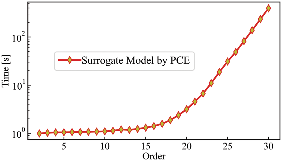
Figure 14: Time required to construct surrogate models of order 2 to 30 using the PCE method

In addition, the normalization is first performed in PCE box to reduce the influence of the range of the independent variables on the fitting effect and improve the performance of the polynomial chaos expansion algorithm. In this example, CV = 8.07% on the test set with the original training set without the normalization of the independent variables, while CV = 4.76% on the test set with the normalized training samples, which means a better fitting effect.

Another three sensitivity analysis of dielectric 5-bladed gear under TM-polarized incident plane wave is carried out here (see Table 2). The surrogate models are constructed with the adaptive PCE method considering the bistatic angle θ, permittivity ε, and the frequency f as the independent variables respectively. These models are applied to depict sensitivity curves (as shown in Figs. 15 and 16) and to obtain the sensitivity average, which is compared with FDM.

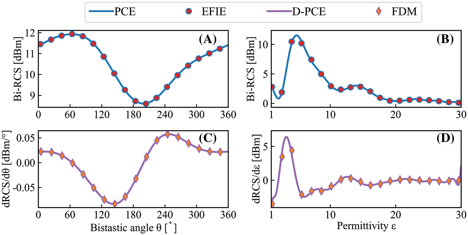
Figure 15: The PCE and sensitivity results for the 5-bladed gear model under TM polarization. (A) and (C): Case 1, f = 50 MHz, ε = 5; (B) and (D): Case 2, f = 50 MHz, θ=0∘

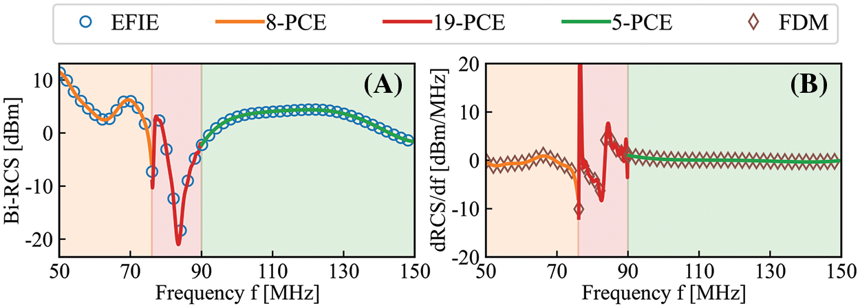
Figure 16: The piecewise fitting results of Case 3 by PCE for the 5-bladed gear model under TM polarization: θ=0∘, ε = 5

It can be seen from Figs. 15 and 16 that the sensitivity information, as well as the original data, could be perfectly expressed by the proposed adaptive PCE method.

For Case 1 and Case 2, the overall change is relatively gentle and the curvature is small, a satisfied surrogate model can be obtained with a low order, which is 4 for Case 1 and 18 for Case 2. The initial value of the training set, the sensitivity value solved by FDM with the training set, the response at the test set with the surrogate model which is constructed using the training set, and the derivatives of the surrogate model at the test set are shown in Fig. 15. It can be seen that the surrogate model constructed by the PCE method can well express the sensitivity information of the original data.

The middle segment of Case 3 fluctuates more violently than the other two segments, it is hard to fit the whole range well using a lower order of surrogate model. It is divided into three parts and the PCE method is used to expand the samples. The result is shown in Fig. 16. The changes of the first and third segments are very gentle, and it is only necessary to use the 8th-order and 5th-order polynomial matrix respectively to construct satisfied surrogate models. The derivative explicit expression can also perform very well on the test set. The data of Case 3-2 changes dramatically. By encrypting the training data points and increasing the order, the 19-order PCE method can be used to construct a surrogate model that meets the requirements. The sensitivity represents the extent of RCS variation within a specific range of independent variables. The greater its absolute value, the more pronounced the change in RCS. It is quite large sometimes because of that the Bi-RCS changes dramatically at this point. In Fig. 16A, the RCS changes dramatically at the frequency of 76 MHz. Correspondingly, in Fig. 16B, the sensitivity value at this point is large.

The statistical characteristics of the sensitivity results by the FDM and 20th-order PCE methods are shown in Table 3, where the relative error is calculated by |Mean(MoM)−Mean(PCE)Mean(MoM)|×100%. Combined with the previous results, the more drastic the bistatic RCS curve changes, the larger the fitting error of statistical features is, but all of them are at a low level. In addition, 0.13>0.106>0.0001. It can be concluded that within θ∈[0,360]∘,ε∈[1,30], f∈[50,150] MHz, the RCS is more sensitive to the frequency f and the permittivity ε.

Based on the above conclusions, taking frequency f and permittivity ε as the sources of system uncertainty, and using the results of the MoM as the input data of the PCE box, a multivariate surrogate model of electromagnetic scattering sensitivity is constructed, which is compared with the analytical solution of the cylinder model. The radius is 1, the bistastic angle θ=0∘, the frequency f∈[30,50] MHz, and the permittivity ε∈[4,6]. The number of training sets is 1681, and the number of testing sets is 10000. The generalized 2-D FDM is used to calculate the sensitivity of bivariate analysis as Eq. (28).

di,j=(yi+1,j+1−yi+1,juj+1[2]−uj[2]−yi,j+1−yi,juj+1[2]−uj[2])/(ui+1[1]−ui[1])=(yi+1,j+1+yi,j)−(yi+1,j+yi,j+1)(ui+1[1]−ui[1])⋅(uj+1[2]−uj[2])(28)

where the di,j denotes the sensitivity of bistatic RCS units in row i and column j, ui[l] represents the coordinate value at the i-th point of the normalized sequence u[l].

Fig. 17 illustrates the bi-RCS and sensitivity results of the PCE method with order = 5, 10, 15. It can be seen that with the increase of the order, the shape of the error map is similar, but the height is significantly decreased in general, and the yellow area is significantly reduced, which indicates that increasing the order works for improving the fitting effect and the prediction accuracy. The CV of sensitivity results between the analytical and the 15th-order PCE-MoM is 1.67%. However, a small range increase of the order has limited ability to reduce the error in a narrow region with a sharp mutation.

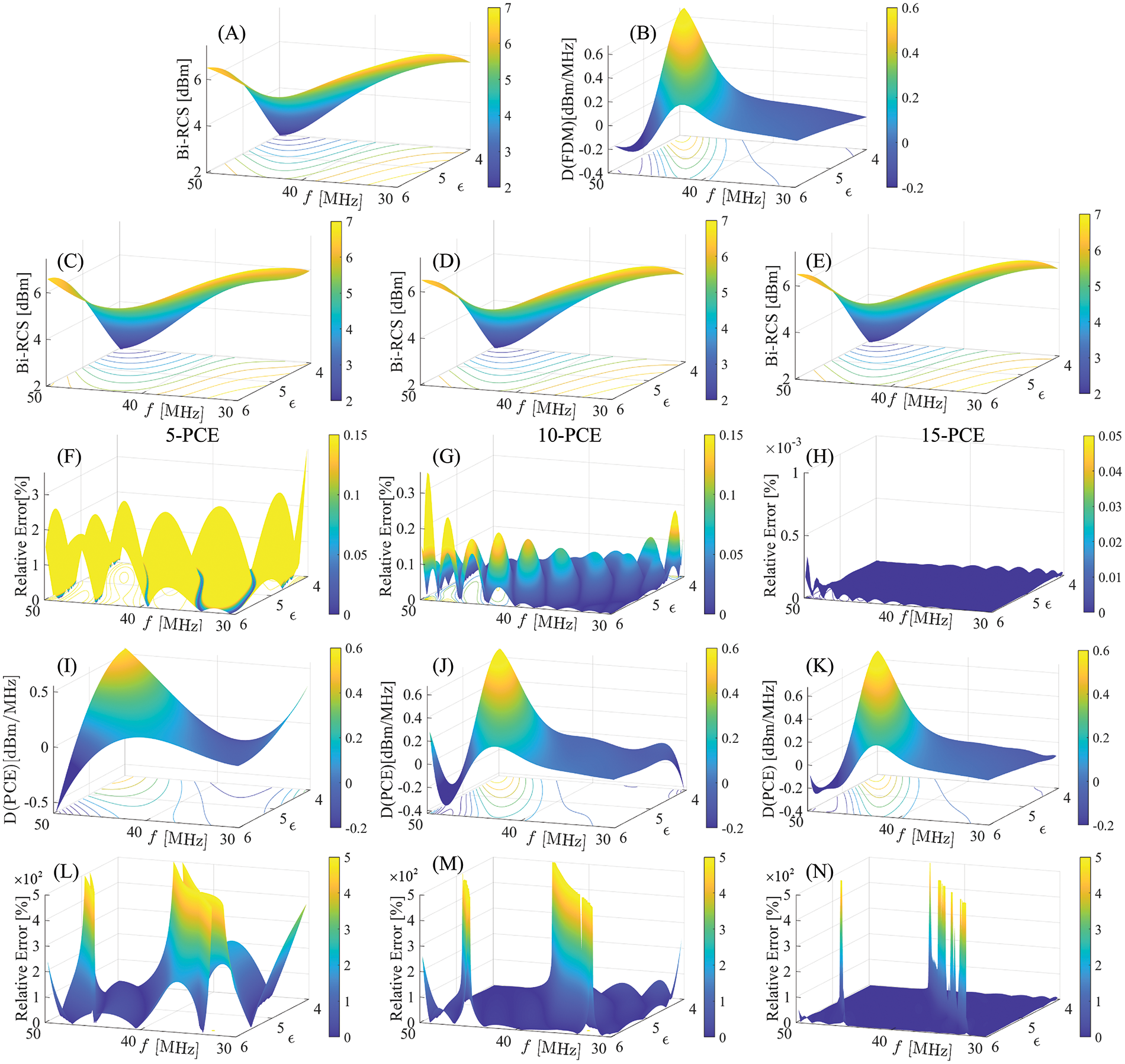
Figure 17: The results using PCE with the electromagnetic scattering test set for the cylinder model: θ=0∘, f∈[30,50] MHz, ε∈[4,6], order = 5, 10, 15; TE polarization. (A) The bi-RCS by the analytical method; (B) The sensitivity by gFDM; (C–E) Bi-RCS by PCE-MoM; (F–H) The relative error between the analytical solution and the PCE-MoM results. (I–K) The sensitivity by PCE-MoM. (L–N) The relative error between gFDM and the PCE-MoM results

Using the method of moments, the time needed to calculate 10000 test samples is 48084.78 s, and the time to calculate 1681 groups of training samples is 8091.05 s, while the time used to build the two-dimensional 15th-order surrogate model by PCE is 215 s, which greatly reduces the calculation time of data expansion.

5  Conclusion

This paper presents a sensitivity analysis method for homogeneous dielectric targets. The triangle functions are utilized to discretize and test the EFIE, and the fictitious current on the dielectric surface is obtained by solving the coefficients. The RCS samples obtained from MoM considering several different variables are subsequently divided into the training set and the testing set and inputted into the adaptive PCE box. CV <5% is used as the exit condition of the order loops. The normalization method is used to improve the performance of the PCE method.

Numerical examples show that the Bi-RCS is sensitive to frequency and permittivity. The correctness and efficiency of the proposed sensitivity analysis method for electromagnetic scattering are verified by comparing with the results obtained by the MoM, analytical solutions, and FDM. The accuracy of the surrogate model is affected by the number of training samples, the order of the model, and the complexity of the model. The calculation time is mainly related to the order, so the calculation cost and accuracy can be balanced by improving the sample quality or fitting the complex interval piecewise. This method can efficiently acquire large-scale samples in the bounded range. We believe that this framework is user-friendly and conducive to future development.

In future research, the proposed technique will be optimized and extended to address three-dimensional electromagnetic problems, further enhancing its versatility and applicability across various engineering fields.

Acknowledgement: The authors wish to express their appreciation to the reviewers for their helpful suggestions which greatly improved the presentation of this paper.

Funding Statement: This work was supported by the Young Scientists Fund of the National Natural Science Foundation of China (No. 62102444) and a Major Research Project in Higher Education Institutions in Henan Province (No. 23A560015).

Author Contributions: The authors confirm contribution to the paper as follows: study conception and design: Yujing Ma, Xiaohui Yuan; data collection: Zhongwang Wang, Ruijin Huo; analysis and interpretation of results: Zhongwang Wang, Jieyuan Zhang, Yujing Ma; draft manuscript preparation: Yujing Ma, Xiaohui Yuan, Jieyuan Zhang. All authors reviewed the results and approved the final version of the manuscript.

Availability of Data and Materials: Data is available on request.

Conflicts of Interest: The authors declare that they have no conflicts of interest to report regarding the present study.

References

1. Taflove A, Hagness S. Computational electrodynamics: the finite-difference time-domain method. 3rd edition. Boston: Artech House Publisher; 2005. [Google Scholar]

2. Gedney S. The finite element method in electromagnetics. IEEE Antennas Propag Mag. 1994;36(7):75–6. [Google Scholar]

3. Jin J. The finite element method in electromagnetics. New Jersey: Wiley-IEEE Press; 2015. [Google Scholar]

4. Shen X, Du C, Jiang S, Zhang P, Chen L. Multivariate uncertainty analysis of fracture problems through model order reduction accelerated SBFEM. Appl Math Modell. 2024;125:218–40. doi:https://doi.org/10.1016/j.apm.2023.08.040. [Google Scholar] [CrossRef]

5. Cao G, Yu B, Chen L, Yao W. Isogeometric dual reciprocity BEM for solving non-Fourier transient heat transfer problems in FGMs with uncertainty analysis. Int J Heat Mass Transfer. 2023;203:123783. doi:https://doi.org/10.1016/j.ijheatmasstransfer.2022.123783. [Google Scholar] [CrossRef]

6. Lu C, Chen L, Luo J, Chen H. Acoustic shape optimization based on isogeometric boundary element method with subdivision surfaces. Eng Anal Boundary Elem. 2023;146:951–65. doi:https://doi.org/10.1016/j.enganabound.2022.11.010. [Google Scholar] [CrossRef]

7. Zhang Y, Li E. Scattering of three-dimensional chiral objects above a perfect conducting plane by hybrid finite element method. J Electromagn Waves Appl. 2005;19(11):1535–46. doi:https://doi.org/10.1163/156939305775701813. [Google Scholar] [CrossRef]

8. Chen L, Wang Z, Peng X, Yang J, Wu P, Lian H. Modeling pressurized fracture propagation with the isogeometric BEM. Geomech Geophys Geo Energy Ge Resour. 2021;7(3):51–61. doi:https://doi.org/10.1007/s40948-021-00248-3. [Google Scholar] [CrossRef]

9. Chen L, Zhang Y, Lian H, Atroshchenko E, Ding C, Bordas SPA. Seamless integration of computer-aided geometric modeling and acoustic simulation: isogeometric boundary element methods based on Catmull-Clark subdivision surfaces. Adv Eng Softw. 2020;149:102879. doi:https://doi.org/10.1016/j.advengsoft.2020.102879. [Google Scholar] [CrossRef]

10. Chen L, Lian H, Xu Y, Li S, Liu Z, Atroshchenko E, et al. Generalized isogeometric boundary element method for uncertainty analysis of time-harmonic wave propagation in infinite domains. Appl Math Modell. 2023;114:360–78. doi:https://doi.org/10.1016/j.apm.2022.09.030. [Google Scholar] [CrossRef]

11. Muhammad N, Ahmed N. Method of moments solution to ethylene glycol based Al2O3 nanofluid flow through expanding/contracting rectangular channel. Heliyon. 2023;9(12):22415. doi:https://doi.org/10.1016/j.heliyon.2023.e22415. [Google Scholar] [PubMed] [CrossRef]

12. Chen L, Lian H, Liu Z, Chen H, Atroshchenko E, Bordas SPA. Structural shape optimization of three dimensional acoustic problems with isogeometric boundary element methods. Comput Methods Appl Mech Eng. 2019;355:926–51. doi:https://doi.org/10.1016/j.cma.2019.06.012. [Google Scholar] [CrossRef]

13. Lian H, Kerfriden P, Bordas SPA. Implementation of regularized isogeometric boundary element methods for gradient-based shape optimization in two-dimensional linear elasticity. Int J Numer Methods Eng. 2016;106(12):972–1017. doi:https://doi.org/10.1002/nme.5149. [Google Scholar] [CrossRef]

14. Chen L, Lu C, Lian H, Liu Z, Zhao W, Li S, et al. Acoustic topology optimization of sound absorbing materials directly from subdivision surfaces with isogeometric boundary element methods. Comput Methods Appl Mech Eng. 2020;362:112806. doi:https://doi.org/10.1016/j.cma.2019.112806. [Google Scholar] [CrossRef]

15. Chen L, Lian H, Liu Z, Gong Y, Zheng CJ, Bordas SPA. Bi-material topology optimization for fully coupled structural-acoustic systems with isogeometric FEM-BEM. Eng Anal Boundary Elem. 2022 Feb 2;135:182–95. doi:https://doi.org/10.1016/j.enganabound.2021.11.005. [Google Scholar] [CrossRef]

16. Chen L, Liu C, Zhao W, Liu L. An isogeometric approach of two dimensional acoustic design sensitivity analysis and topology optimization analysis for absorbing material distribution. Comput Methods Appl Mech Eng. 2018;336:507–32. doi:https://doi.org/10.1016/j.cma.2018.03.025. [Google Scholar] [CrossRef]

17. Liu Z, Bian P, Qu Y, Huang W, Chen L, Chen J, et al. A Galerkin approach for analysing coupling effects in the piezoelectric semiconducting beams. Eur J Mech A Solids. 2024;103:105145. doi:https://doi.org/10.1016/j.euromechsol.2023.105145. [Google Scholar] [CrossRef]

18. Lian H, Chen L, Lin X, Zhao W, Bordas SPA, Zhou M. Noise pollution reduction through a novel optimization procedure in passive control methods. Comput Model Eng Sci. 2022;131(1):1–18. doi:https://doi.org/10.32604/cmes.2022.019705. [Google Scholar] [CrossRef]

19. Zhu W, Zhao R, Zhang Y, Hu J. Analyzing electromagnetic scattering from complex multi-layer patch objects using a multi-trace domain decomposition method. Eng Anal Boundary Elem. 2024;158:468–72. doi:https://doi.org/10.1016/j.enganabound.2023.11.019. [Google Scholar] [CrossRef]

20. Nie X, Yuan N, Li J, Gan YB, Yeo R. A fast volume-surface integral equation solver for scattering from composite conducting-dielectric objects. IEEE Trans Antennas Propag. 2005;53(3):818–24. doi:https://doi.org/10.1109/TAP.2004.841323. [Google Scholar] [CrossRef]

21. Ergül Ö, Gürel L. Novel electromagnetic surface integral equations for highly accurate computations of dielectric bodies with arbitrarily low contrasts. J Comput Phys. 2008;227(23):9898–912. doi:https://doi.org/10.1016/j.jcp.2008.08.004. [Google Scholar] [CrossRef]

22. Ergul O, Gurel L. Comparison of integral equation formulations for the fast and accurate solution of scattering problems involving dielectric objects with the multilevel fast multipole algorithm. IEEE Trans Antennas Propag. 2009;57:176–87. doi:https://doi.org/10.1109/TAP.2008.2009665. [Google Scholar] [CrossRef]

23. Chen L, Lian H, Natarajan S, Zhao W, Chen X, Bordas SPA. Multi-frequency acoustic topology optimization of sound-absorption materials with isogeometric boundary element methods accelerated by frequency-decoupling and model order reduction techniques. Comput Methods Appl Mech Eng. 2022;395:114997. doi:https://doi.org/10.1016/j.cma.2022.114997. [Google Scholar] [CrossRef]

24. Qu Y, Pan E, Zhu F, Jin F, Roy A. Modeling thermoelectric effects in piezoelectric semiconductors: new fully coupled mechanisms for mechanically manipulated heat flux and refrigeration. Int J Eng Sci. 2023 Jan;182:103775. doi:https://doi.org/10.1016/j.ijengsci.2022.103775. [Google Scholar] [CrossRef]

25. Chen L, Zhao J, Lian H, Yu B, Atroshchenko E, Li P. A BEM broadband topology optimization strategy based on Taylor expansion and SOAR method Application to 2D acoustic scattering problems. Int J Numer Methods Eng. 2023 Aug;124(5):5151–82. doi:https://doi.org/10.1002/nme.7345. [Google Scholar] [CrossRef]

26. Qu Y, Jin F, Yang J. Buckling of a Reissner Mindlin plate of piezoelectric semiconductors. Meccanica. 2022 Oct;57:2797–807. doi:https://doi.org/10.1007/s11012-022-01598-2. [Google Scholar] [CrossRef]

27. Chen L, Wang Z, Lian H, Ma Y, Meng Z, Li P, et al. Reduced order isogeometric boundary element methods for CAD-integrated shape optimization in electromagnetic scattering. Comput Methods Appl Mech Eng. 2024;419:116654. doi:https://doi.org/10.1016/j.cma.2023.116654. [Google Scholar] [CrossRef]

28. Chen L, Li H, Guo Y, Chen P, Atroshchenko E, Lian H. Uncertainty quantification of mechanical property of piezoelectric materials based on isogeometric stochastic FEM with generalized nth-order perturbation. Eng Comput. 2024 Feb;40:257–77. doi:https://doi.org/10.1007/s00366-023-01788-w. [Google Scholar] [CrossRef]

29. Sheng X, Jin J. On the formulation of hybrid finite-element and boundary-integral methods for 3-D scattering. IEEE Trans Antennas Propag. 1998;46(3):303–11. doi:https://doi.org/10.1109/8.662648. [Google Scholar] [CrossRef]

30. Chen L, Lu C, Zhao W, Chen H, Zheng C. Subdivision surfaces boundary element accelerated by fast multipole for the structural acoustic problem. J Theor Comput Acous. 2020;28(9):2050011. doi:https://doi.org/10.1142/S2591728520500115. [Google Scholar] [CrossRef]

31. Hu X, Fang G, Ge Y. Uncertainty propagation of flutter derivatives and structural damping in buffeting fragility analysis of long-span bridges using surrogate models. Struct Saf. 2024;106:102410. doi:https://doi.org/10.1016/j.strusafe.2023.102410. [Google Scholar] [CrossRef]

32. Yuan X, Ma Y, Huang Y, Huo R, Wang Z. The method of moments for electromagnetic scattering analysis accelerated by the polynomial chaos expansion in infinite domains. Front Phys. 2023;11:1178466. doi:https://doi.org/10.3389/fphy.2023.1178466. [Google Scholar] [CrossRef]

33. Chen L, Cheng R, Li S, Lian H, Zheng C, Bordas SPA. A sample-efficient deep learning method for multivariate uncertainty qualification of acoustic-vibration interaction problems. Comput Methods Appl Mech Eng. 2022;393:114784. doi:https://doi.org/10.1016/j.cma.2022.114784. [Google Scholar] [CrossRef]

34. Friedman JH. Multivariate adaptive regression splines. Ann Stat. 1991;19(1):1–67. doi:https://doi.org/10.1214/aos/1176347963. [Google Scholar] [CrossRef]

35. Shen X, Du C, Jiang S, Sun L, Chen L. Enhancing deep neural networks for multivariate uncertainty analysis of cracked structures by POD-RBF. Theor Appl Fract Mech. 2023;125:103925. doi:https://doi.org/10.1016/j.tafmec.2023.103925. [Google Scholar] [CrossRef]

36. Zhang S, Yu B, Chen L. Non-iterative reconstruction of time-domain sound pressure and rapid prediction of large-scale sound field based on IG-DRBEM and POD-RBF. J Sound Vib. 2024 Dec;573:118226. doi:https://doi.org/10.1016/j.jsv.2023.118226. [Google Scholar] [CrossRef]

37. Drucker H, Burges C, Kaufman L, Smola A, Vapnik V. Support vector regression machines. Adv Neural Inform Process Syst. 1997 Jan;28:779–84. [Google Scholar]

38. Rasmussen CE, Williams CKI. Gaussian processes for machine learning. Cambridge: The MIT Press; 2005. [Google Scholar]

39. Wiener N. The homogeneous chaos. Am J Math. 1938;60:897. doi:https://doi.org/10.2307/2371268. [Google Scholar] [CrossRef]

40. Cameron RH, Martin WT. Transformations of wiener integrals under a general class of linear transformations. Trans Am Math So. 1945;58(2):184–219. doi:https://doi.org/10.2307/1990282. [Google Scholar] [CrossRef]

41. Ghanem RG, Spanos PD. Stochastic finite elements: a spectral approach. New York: Springer; 1992. [Google Scholar]

42. Gibson W. The method of moments in electromagnetics. New York: CRC Press; 2021. [Google Scholar]

Appendix A. Analytical Solution

The dielectric infinite cylinder, impinged by electromagnetic plane waves with different polarization directions, is considered and its analytical solutions are obtained in this section.

The scattered electric field under TE-polarized incident waves can be expressed as

Escaz(ρ,θ)=∑n=0∞incnAnDIEHn(2)(k0ρ)cos⁡(nθ)(29)

where |Escaz|=1 for convenience, θ is the bistatic angle, and cn = 1 for n = 0, and cn = 2 otherwise. The series coefficients AnDIE could be expressed as

AnDIE=−(k1/μ2)Jn(k0r)Jn ′(k1r)−(k0/μ1)Jn ′(k0r)Jn ′(k1r)(k1/μ2)Hn(2)(k0r)Jn ′(k1r)−(k0/μ1)Hn ′(2)(k0r)Jn ′(k1r)(30)

where r is the radius of the cylinder. The induced electric current Jz(ϕ) is

Jz(ϕ)=2πη0k0r∑n=0∞(j)ncncos(nϕ)Hn(2)(k0r)(31)

where ϕ is the azimuthal angle on the surface of the cylinder.

The expression of the scattered magnetic field under TM polarization is obtained by

Hzsca(ρ,θ)=1η0∑n=0∞incnBnDIEHn(2)(k0ρ)cos⁡(nθ)(32)

where Hscaz means the scattered magnetic field with a z-directed incident magnetic field. |Einc|=1 for convenience. The coefficients BnDIE for TM polarization are

BnDIE=−(k1/ε1)Jn(k0r)Jn ′(k1r)−(k0/ε0)Jn ′(k0r)Jn ′(k1r)(k1/ε1)Hn(2)(k0r)Jn ′(k1r)−(k0/ε0)Hn ′(2)(k0r)Jn ′(k1r)(33)

The induced azimuthal electric current is

Jz(ϕ)=2jπη0k0r∑n=0∞(j)ncncos(nϕ)Hn ′(2)(k0r)ϕ^(34)

The recurrence relationship Zn ′(ka)=nkaZn(ka)−Zn+1(ka) can be used to compute the derivatives.