Development of a Three-Dimensional Multiscale Octree SBFEM for Viscoelastic Problems of Heterogeneous Materials

Nomenclature

1  Introduction

Heterogeneous viscoelastic materials, such as concrete [1] and polymers [2], are widely used in many fields because of their excellent properties. The macroscopic responses of these heterogeneous materials are known to be significantly influenced by physical phenomena at different scales and the interaction between different scales [3].

The Direct Numerical Simulation (DNS) method, usually implemented by the Finite Element Method (FEM) [4–6], is widely used to effectively determine the mechanical responses of heterogeneous viscoelastic materials. However, the DNS method could incur high computational costs and become impractical for numerical analysis of whole structures due to the tremendous amount of computer memory and CPU time needed to mesh all heterogeneities [7].

Compared with the DNS method, the multiscale methods can effectively reduce the degree of freedoms (DOFs) of numerical analysis on a coarse-scale mesh without resolving all small-scale features [8,9]. There are a large number of multiscale methods in literature, including analytical models and computational multiscale methods. The analytical models focus on obtaining equivalent performance on a large scale, including variational principles [8–10], self-consistent methods [11–13] and Mori-Tanaka methods [14–16], etc. Although these methods work well to predict the equivalent properties of heterogeneous materials with a small volume fraction and simple geometry, most of these methods contain over-ideal assumptions [17]. To address this issue, the numerical models were developed and became more popular, including asymptotic homogenization methods [18–20], computational homogenization methods [21–24] and FE2 methods [25–28]. However, these methods have some limitations including the assumption of scale separation and periodicity. The multiscale finite element method (MsFEM) presented by Babuška et al. [29,30] is another computational multiscale method. The basic idea of the MsFEM is to construct a bridge between different scales via the numerical base functions [31–33], and the MsFEM can deal with non-periodic continuum problems. The MsFEM was firstly used to solve scalar field problems [34] and has been successfully applied in various heterogeneous multiscale analyses related to dynamic problems [35], elastic-plastic problems [36], and thermal-mechanical coupling problems [37].

To reproduce more realistic situations for heterogeneous viscoelastic analysis, it is desirable to develop three-dimensional multiscale approaches under the framework of MsFEM, as the problems in practical applications are general in 3D cases. However, most of the aforementioned works on MsFEM are limited to two-dimensional cases. Klimczak et al. presented a three-dimensional MsFEM for viscoelastic problems, in which conventional FEM is used for the three-dimensional base function in small-scale [38]. However, the calculation of numerical base functions by conventional FEM could be very time-consuming due to a large number of degrees of freedom (DOFs) when complex microstructures exist in small-scale. Besides, for the microstructures with material heterogeneity, the three-dimensional mesh generation in small-scale could be also very complex as the conforming conditions on the element/material interfaces are required to be satisfied in transition of different mesh densities [39].

The Scaled Boundary Finite Element Method (SBFEM) originally presented by Song et al. [40] is a semi-analytical method for solving partial differential equations. The SBFEM is particularly suitable for stress singularities and unbounded domain and it has been widely applied into fracture problems [41,42], dynamics problems [43,44], uncertainty analysis [45,46], optimization problems [47,48], and parallel computations [49,50]. Recently, the quadtree/octree SBFEMs have been successfully developed by virtual of the ability of SBFEM to build polygonal elements [51–53]. In our previous works [54,55], a Multiscale Scaled Boundary Finite Element Method (MsSBFEM) was proposed by integrating the advantages of quadtree SBFEM and MsFEM, in which the numerical base functions in small-scale are calculated by SBFEM instead of conventional FEM. However, these works have only addressed two-dimensional problems, which cannot accurately reflect realistic conditions in many cases. In order to apply the MsSBFEM into more realistic problems with complex geometries, materials distribution and, boundary conditions, a three-dimensional MsSBFEM for heterogeneous viscoelastic materials is further developed by extending the previous basic two-dimensional method. In the proposed method, the octree SBFEM is used to deal with the three-dimensional calculation of numerical base functions in small-scale. The Octree-SBFEM has been applied in elastic [56], elastic-plastic [57], and sound field problems [58] including the development of cutting mesh technique [59] and polyhedral mesh [60–62] to handle the complex 3D boundary interfaces. However, to the authors’ best knowledge, it is the first time to develop the three-dimensional MsSBFEM with octree mesh and apply it to the multiscale viscoelastic analysis. The proposed method has the following advantages:

(1) Using the numerical base function in the framework of the MsFEM, a bridge between the small-scale and large-scale is established. In this way, the DOFs of numerical computations for three-dimensional viscoelastic problems can be significantly reduced compared with those of DNS.

(2) The numerical base functions in the proposed model are constructed via image-based analysis based on the octree SBFEM instead of the conventional FEM with twofold advantages. First, the mesh can be directly generated from three-dimensional images on a small-scale without a requiring complex geometric modeling process in conventional FEM. Second, the stiffness matrix can be directly assembled through extraction from several basic patterns of three-dimensional elements to speed up the multiscale analysis [63,64].

(3) The Temporally Piecewise Adaptive Algorithm (TPAA) is used for discretization in the time domain for three-dimensional viscoelastic analysis [65–67]. In this way, a prescribed accuracy in the time domain can be maintained by adaptively changing the recursive order without the assumption that variables remain constant or change linearly at a discretized time interval.

The paper is organized as follows. Section 2 introduces the basic framework of the MsFEM and the construction process of three-dimensional numerical base functions based on the octree SBFEM is presented. Section 3 introduces the solution of viscoelastic problems based on the TPAA and its implementation in the framework of a three-dimensional multiscale SBFEM. Section 4 demonstrates the effectiveness of the proposed method via three numerical examples, and Section 5 presents some concluding remarks and discussions of future work.

2  Key Equation of the 3D Multiscale Octree SBFEM for Elastic Problems

2.1 The Introduction on the Framework of MsFEM

The equilibrium equation with boundary conditions for elastic problems can be expressed as [66]

Hσ+F=0in ΩE(1)

u=uΓonΓu(2)

p=pΓonΓσ(3)

where σ, ε and u represent the vectors of stress, strain, and displacement, respectively, F is the vector of body force intensities, ΩE denotes the spatial domain to be solved, and H is the differential operator [65]. uΓ and pΓ are the prescribed vectors along the displacement boundary Γu and stress boundary Γσ, respectively.

The strain vector is expressed as

ε=HTu(4)

The constitutive equation is

σ=Dε(5)

where D is the elastic matrix.

According to the basic idea of the MsFEM, a three-dimensional domain can have two levels of meshes as shown in Fig. 1, i.e., the coarse elements on a large-scale and the fine elements on a small-scale. The subscript E indicates that the variable belongs to the large-scale element. The FEM equation for solving the nodal displacement on coarse elements uE is written as

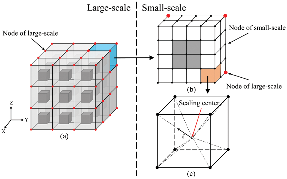
Figure 1: Meshes in 3D MsSBFEM (a) coarse grids on overall structure (b) fine grids inside the coarse element (c) octree SBFEs

KGuE=PG(6)

where KG and PG are the global stiffness matrix and load vector of the large-scale assembled of all coarse elements. These can be written as

KG=Aj=1RKjE(7)

PG=Aj=1RPjE(8)

where Aj=1R is the assembly operator, KjE and PjE are the stiffness matrix and load vector of the j-th coarse element, respectively, and R is the total number of coarse elements.

Instead of using regular numerical integration calculations, the KjE and PjE are obtained by a mapping relationship from the corresponding matrix or vector of fine elements inside this coarse element as [36]

KjE=∑i=1rGjTKieGj(9)

PjE=∑i=1rGjTPie(10)

where Gj is the transfer matrix, r is the total number of fine elements, and the subscript e indicates that the variable belongs to the small-scale element. In this way, this elastic problem is solved on a large-scale, so the number of DOFs is significantly reduced compared to DNS in small-scale. In the following section, we introduce how to establish Gj.

2.2 Octree SBFEM Based Numerical Base Functions

The three-dimensional displacement fields within the j-th coarse element can be expressed as [36]

uie=GiujE(11)

where Gi is the transfer matrix of the i-th fine element, and uie and ujE are the nodal displacement vectors for the j-th coarse element and the i-th fine element inside this coarse element, respectively.

Gi in Eq. (11) is composed of numerical base functions Nn as

Gi=[N1xi(1)N1yi(1)N1zi(1)…NIxi(1)NIyi(1)NIzi(1)N1xi(2)N1yi(2)N1zi(2)…NIxi(2)NIyi(2)NIzi(2)…………………N1xi(n)N1yi(n)N1zi(n)…NIxi(n)NIyi(n)NIzi(n)](12)

where

NIxi(n)=[NIxxi(n)NIyxi(n)NIzxi(n)]T(13)

NIyi(n)=[NIxyi(n)NIyyi(n)NIzyi(n)]T(14)

NIzi(n)=[NIxzi(n)NIyzi(n)NIzzi(n)]T(15)

where n and I are the numbers of nodes in the fine element and coarse element, respectively. Taking NIyzi(n) as an example, Eqs. (13)–(15) indicate that the displacement of the I-th node of the j-th coarse element in the z direction leads to the displacement of the n-th node in the y direction of the i-th fine element.

NIxi, NIyi and NIzi are solved in the same governing equations but with different boundary conditions for the fine elements shown in Fig. 1b. Taking NIzi as an example, the governing equations and boundary conditions can be written as

H(DHTNIzi)=0inΩE(16)

NIzi=NIzionΓE(17)

I=1,2,…,R(18)

where R is the nodal number of a coarse element and D is the elastic matrix.

In this paper, the linear boundary conditions are considered [34] as shown in Fig. 2, which means that we calculate NIzi with I = 1, the boundary conditions are set as N1zi=1 and N2zi=N3zi=…=N8zi=0, and the z-direction displacement NIzi is assumed to be a linear change on the Surface 1, Surface 3, and Surface 5, as well as the lines 12, 14 and 15 on these surfaces. When constructing the numerical basis function in the z-direction, the displacements in the x-direction, y-direction and on all boundaries are fully constrained. The NIxi and NIyi in the x-direction and y-direction can be constructed similarly.

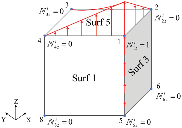
Figure 2: 3D liner boundary conditions for numerical base function of displacement field

The governing equations for the numerical base functions in Eqs. (16) and (17) are solved using the SBFEM with an octree mesh on a fine grid in the small-scale [55]. The generation of the octree mesh and the computational scheme for the three-dimensional SBFEM are introduced in the following sections and the Appendix.

2.3 Image-Based Octree Gridding Technique

In order to solve the numerical base functions introduced in Section 3.1, the octree mesh is used in the SBFEM based calculation. The octree mesh can be directly generated from 3D images in small-scale. A detailed introduction of this approach is provided in reference [63] and an example is shown in Fig. 3. Firstly, a 3D image, usually obtained from imaging techniques such as X-ray computed tomography (XCT) or produced digitally via random generation and packing of aggregates, is read to produce a 3D image matrix containing information on color intensity. Secondly, the octree decomposition is implemented to recursively divide a 3D image matrix into eight equal-sized cells at a time until all the cells satisfy the criterion of homogeneity or the minimum edge length is reached.

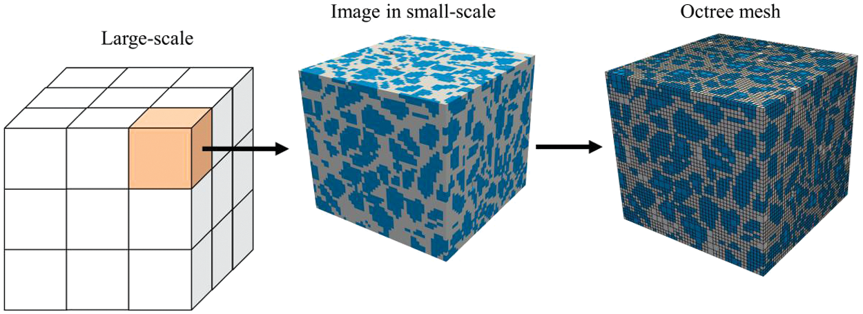
Figure 3: Image based 3D multiscale mesh generation

When a 2:1 rule is used in the process of octree gridding, a balanced decomposition can be obtained to limit the number of nodal patterns of one octree mesh. This has significant advantages, as similar nodal patterns can be precomputed because the element matrices for two octree cells with equivalent nodal configurations are proportional. In such a balanced decomposition, each element mode only depends on whether there is a hanging node in the center of each edge of the cube, and if there are four hanging nodes on any surface of the cube (as shown in Fig. 4), the node in the center of the surface will be automatically added, and it is proved that the number of total unique nodal patterns for an octree cell is 212=4096 [63].

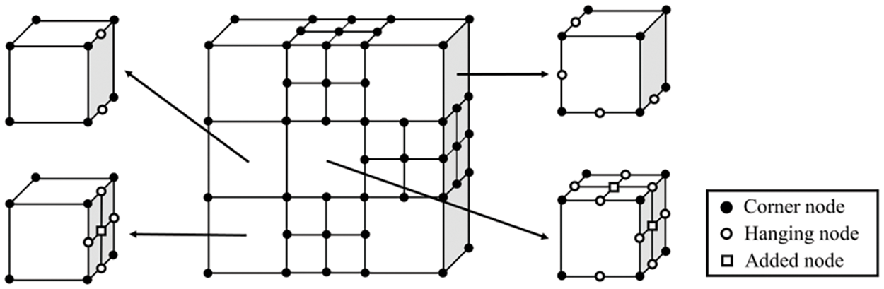
Figure 4: Several typical three-dimensional octree scaled boundary elements

3  Recursive 3D Multiscale Octree SBFEM for Viscoelastic Problems

3.1 Recursive Governing and Constitutive Equations

To handle time-dependent viscoelastic problems, the discretization in the time domain is achieved using the Temporally Piecewise Adaptive Algorithm (TPAA) [66], in which all variables are expanded in each time as follows:

f(t)=∑m=0fmsm(19)

where the general variable f(t) is used to represent σ(t), ε(t), F(t), u(t), uΓ(t), p(t) and pΓ(t) in Eqs. (1)–(5), and

s=t−tk−1Tk(20)

where t and s denote the time and dimensionless time parameters, respectively, and tk−1 and Tk are the initial point and size of the kth time interval, respectively.

Substituting the expanded variables into Eqs. (1)–(3), we have the following governing equations for the expansion coefficients

Hσm+Fm=0in Ω(21)

εm=HTum(22)

um=uΓmonΓu(23)

pm=pΓmonΓσ(24)

Now, we derive the recursive constitutive relationship for σ(t) and ε(t). In this paper, we consider the three-parameter solid model as a typical viscoelastic constitutive model, as shown in Fig. 5. The differential form of the constitutive equation is written as [67]

{σ(t)+q1∂σ(t)∂t=D(q2ε(t)+q1∂ε(t)∂t)(t>0)σ(t)=Dε(t)(t=0)(25)

where

q1=η1E1+E2;q2=E1E1+E2(26)

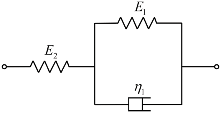
Figure 5: Three-parameter solid model

Considering the relationship between the differentiations with respect to t and s in Eq. (20)

d(⋅)dt=1Tkd(⋅)ds(27)

Therefore, the time derivatives of the stress and strain can be expressed as

∂σ(t)∂t=∑m=0m+1Tkσm+1sm(28)

∂ε(t)∂t=∑m=0m+1Tkεm+1sm(29)

In each time interval, substituting Eqs. (28) and (29), into Eq. (25) and equating the powers of the two sides of the equation yields

σm=Dεm+Cm(30)

where

Cm=Tkm(E1η1Dεm−1−1q1σm−1)(m>0)(31)

At the first time interval,

{σ0=Dε0C0=0(k=1)(32)

At the initial point of the (k+1)th time interval

{εk+10=∑m=0εkmσk+10=∑m=0σkmCk+10=∑m=0Ckm(k>1)(33)

In this way, the time-dependent problems in Eqs. (21)–(25) are transferred into a series of recursive elastic problems with initial stress and strain, which will be recursively solved by the MsSBFEM introduced in the following sections.

3.2 Recursive Multiscale Octree SBFEM for Viscoelastic Problems

Using the derived MsSBFEM equations for elastic problems in Section 2, the recursive governing equations and constitutive equation for three-dimensional viscoelastic problems are naturally solved for coarse elements at large-scale [54].

KG(um)E=PGm(34)

where the right-term PGm contains the term related to Cm in Eq. (31) written as

PGm=Aj=1R[(PSjm)E−(PCjm)E](35)

where

(PSjm)E=∑i=1rGiT(PSjm)e(36)

(PCjm)E=∑i=1r(Gie)T(PCim)e(37)

(PSim)e=∫Γ[Ni(s)]e[Fim(s)]eds(38)

(PCim)e=Tm(−E2iη1iKie(uim−1)e−E1i+E2iη1i(PCim−1)e)(39)

where (uim−1)e is the (m-1)-th order expanding coefficient of the nodal displacement of the i-th fine element.

Note that (uim−1)e and (PCim−1)e in Eq. (39) are obtained via downscale computation from the relationship between two-scale variables using a numerical base function

(uim−1)e=Gi(uim−1)E(40)

(PCim−1)e=Gi(PCim−1)E(41)

The (PCi0)ke at the initial points of the k-th time interval is calculated as

(PCi0)ke=0ifk=1(42)

(PCi0)ke=∑m(PCim)k−1eifk>1(43)

At each time interval, an adaptive computation is conducted by setting the number of expansion terms m following the criteria [67]

‖(um)Esm|s=1‖2‖∑h=0m−1(uh)Esh|s=1‖2≤β(44)

where β is a prescribed error tolerance, and ‖⋅‖2 represents the L2-norm.

4  Numerical Examples

Three numerical examples are provided in this section. The first example demonstrates the effectiveness of the proposed algorithm in a cubic domain with periodic inclusions. The performance of the proposed method for non-periodic inclusions is demonstrated in the second example. The third example applies the proposed method to a concrete beam with CT images of microstructures. To evaluate the accuracy of the proposed method, the relative error er is defined.

4.1 A Cubic Domain with Periodic Inclusions

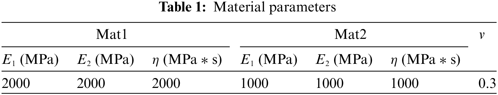
Consider a cube domain of heterogeneous viscoelasticity under tension as shown in Fig. 6. There are 27 small cubic inclusions contained in the cube, and their material parameters are provided in Table 1. In order to investigate the proposed method for different levels of heterogeneity, two cases of volumetric ratios of inclusions κ are set with various sizes a as shown in Fig. 6c, i.e., Case I: a = 42, κ = 28.3%; Case II: a = 50, κ = 47.6%.

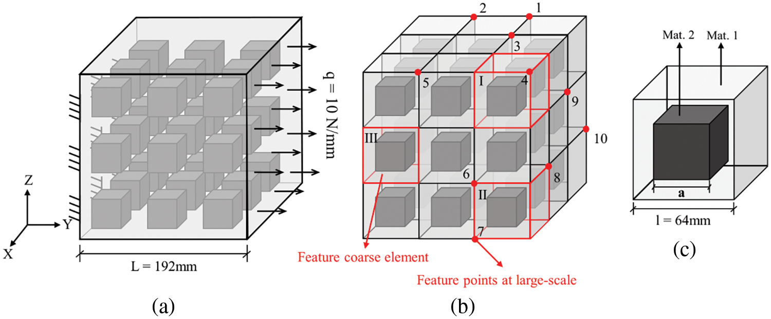
Figure 6: A cube with regular cube inclusions (a) heterogeneous material distribution and boundary conditions (b) coarse mesh (c) the material distribution in one coarse mesh

The material distributions in large-scale and small-scale are shown in Figs. 6b and 7, respectively. In total, 27 uniform coarse elements are used, and three types of coarse elements with different nodal distributions (coarse nodes marked by red color) are used.

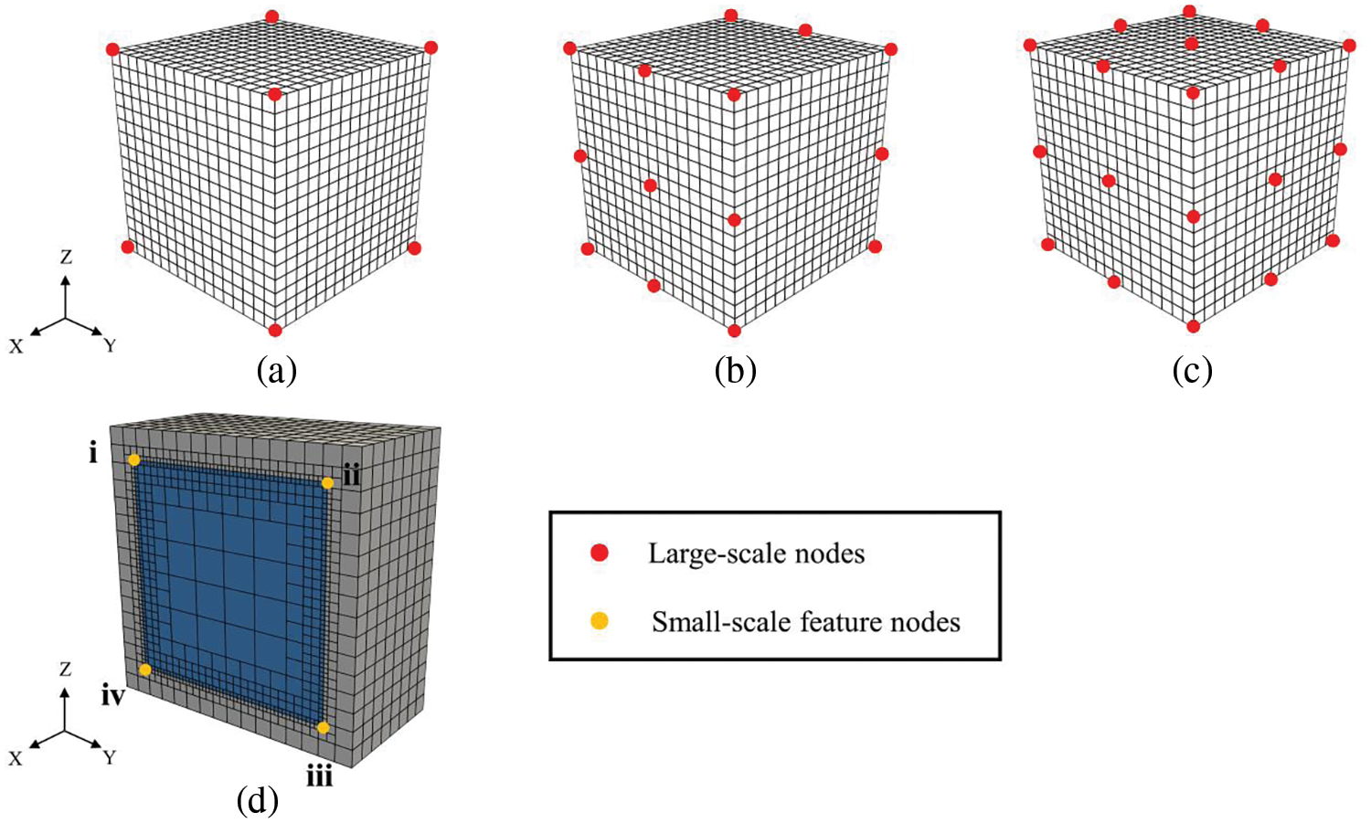
Figure 7: Coarse SBFEs with different number of nodes (a) model A (8 nodes) (b) model B (18 nodes) (c) model C (26 nodes) (d) section view of octree mesh

Firstly, the computational accuracy is verified by comparing the results of the proposed method with the reference solution from a converged Abaqus based DNS solution with its mesh in Fig. 8. Table 2 shows the results of displacement at large-scale feature point 1 (see Fig. 6b) and the results for displacements at small-scale feature point i of coarse element II (see Figs. 6b and 7d) are also provided in Table 3. The maximum relative errors of the proposed method are 0.69% and 0.30% in large-scale and small-scale, respectively, and these relative errors change very slightly when the time step is increased from 0.001 to 0.1 s.

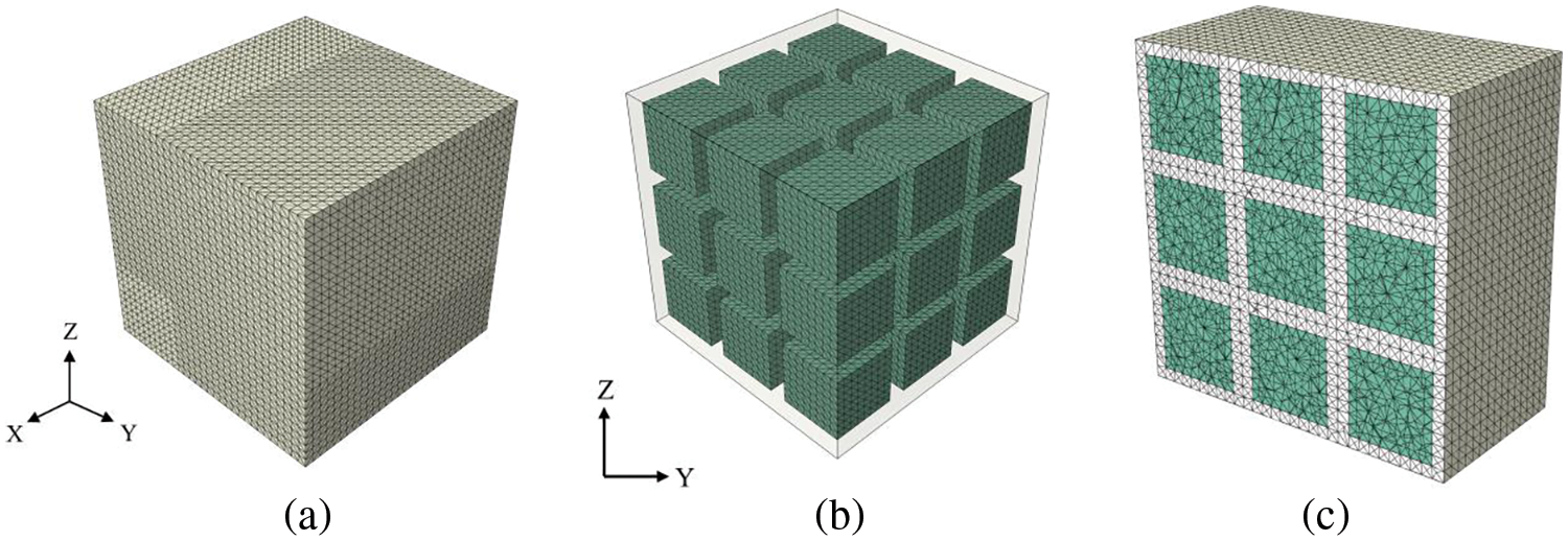
Figure 8: FE mesh of reference solution based on Abaqus (a) matrix (b) inclusions (c) section view

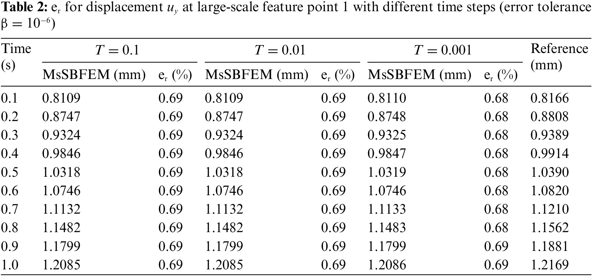
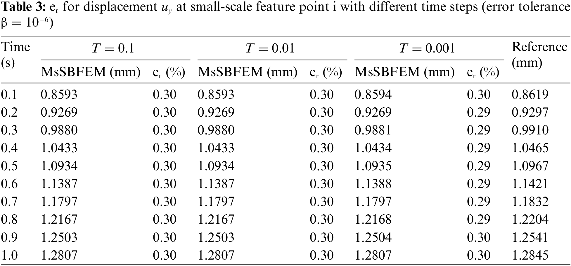
Fig. 9 shows the variation in displacement with time for large-scale feature point 2 and small-scale feature point i in coarse element II. The reference solution is provided by the Abaqus with both automatic and fixed time steps, in which the implicit integration method in the time domain is used. The comparisons of different time steps T = 0.1, 0.01, and 0.001 s are shown in Fig. 9. When the time step of Abaqus is relatively large as T = 0.1 s. Obviously, there are errors in the initial stage, but the proposed method with the same time step still achieves good results which shows that the TPAA algorithm is capable of adaptively adjusting the expansion order to ensure the accuracy in the time domain. Fig. 10 shows the comparison of the expansion order under two different prescribed convergence accuracy parameters, which indicate that the TPAA algorithm can also adaptively adjust the expansion order to balance the calculation accuracy and efficiency when the given convergence accuracy changes.

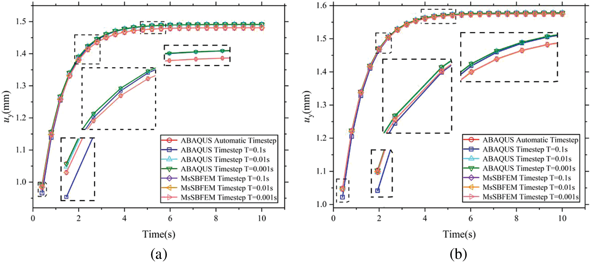
Figure 9: Displacement curves of feature points with different time steps (a) The large-scale feature point 1 (b) The small-scale feature point i in the coarse element II

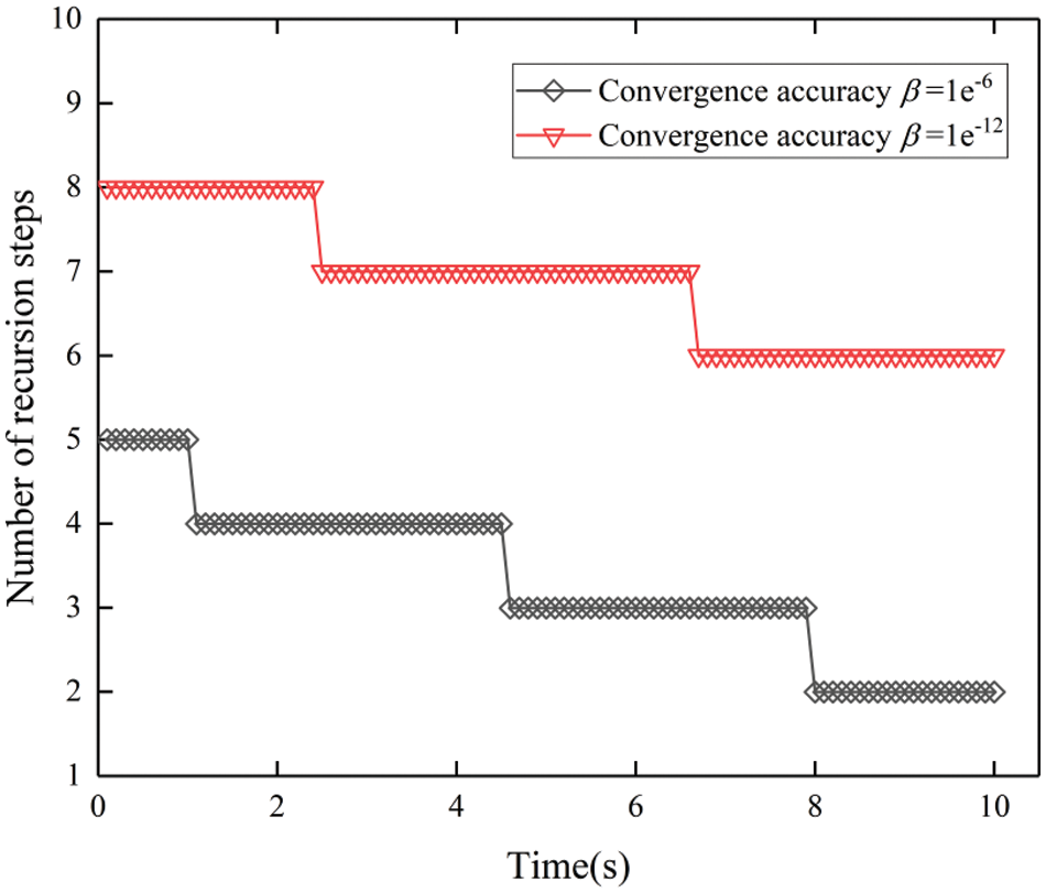
Figure 10: The variation of recursive orders with time

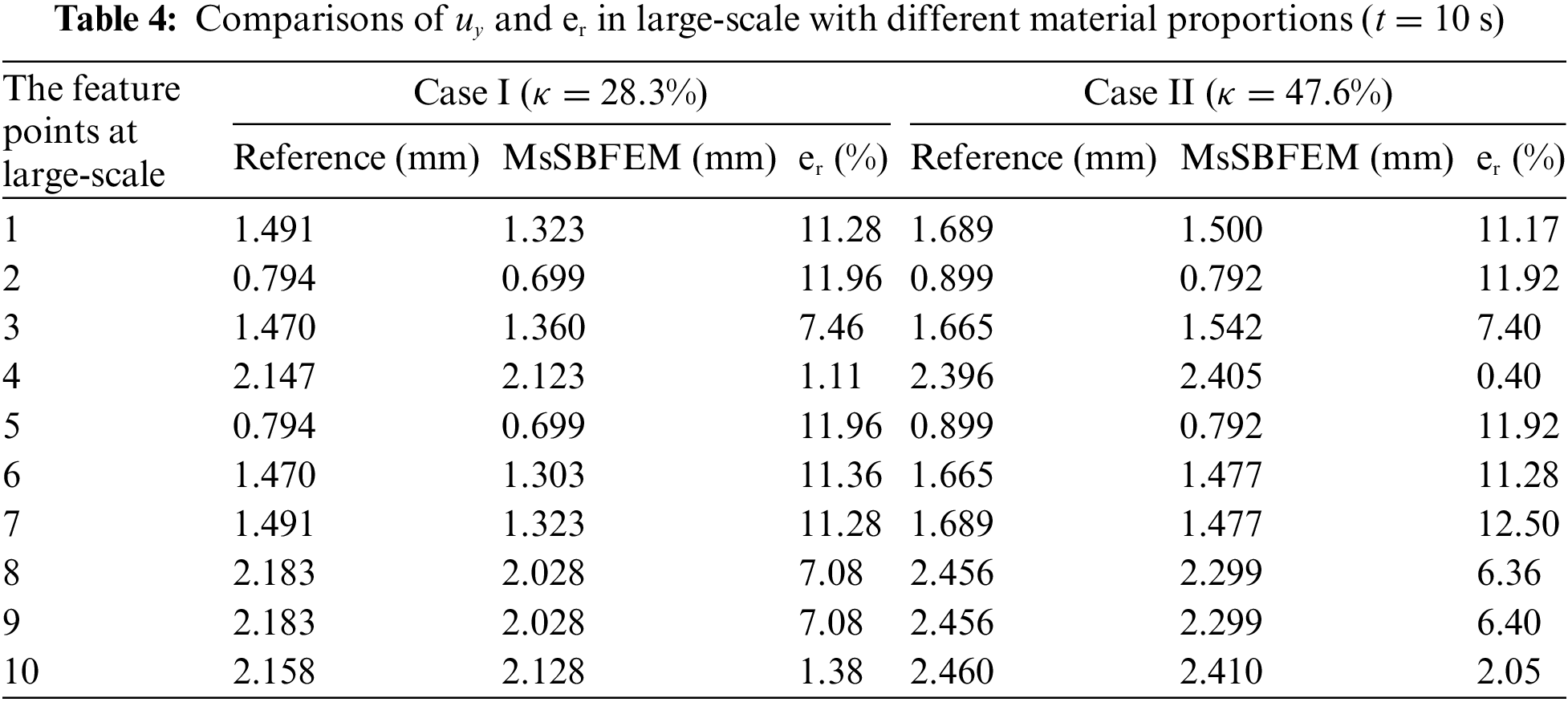
Secondly, the two cases of material properties in case I and case II in Table 1 are tested by using the coarse element Model A with 8 nodes, as shown in Fig. 7. Table 4 shows the results of uy on large-scale feature nodes shown in Fig. 6b when t = 10 s and its relative error er. The calculation results show that for two cases of material properties in case I and case II, although er is less than 3% on nodes 4 and 10, but er on some other nodes are still quite large nearly 10%. We will discuss how to improve the accuracy by adjusting the types of coarse elements in the following section.

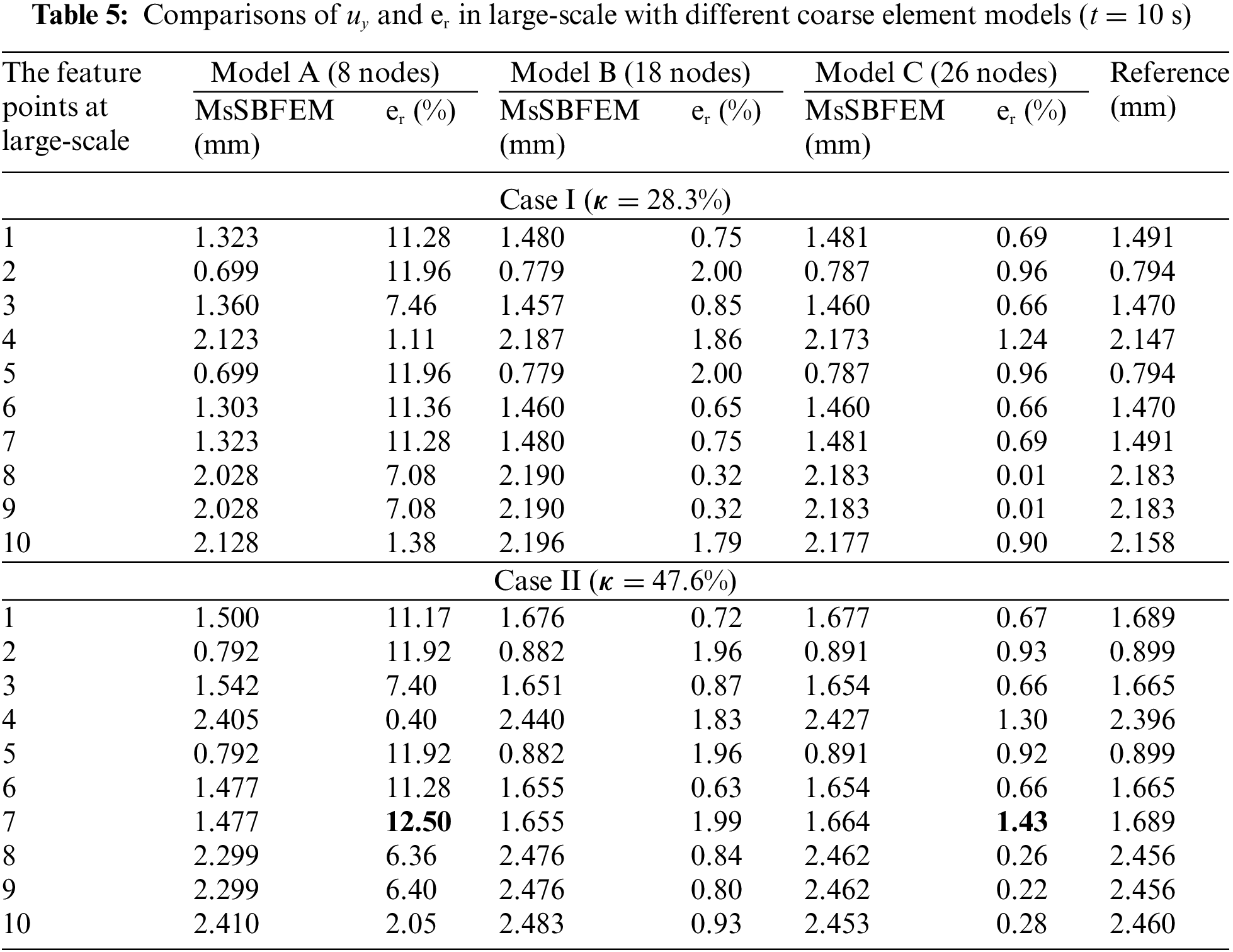
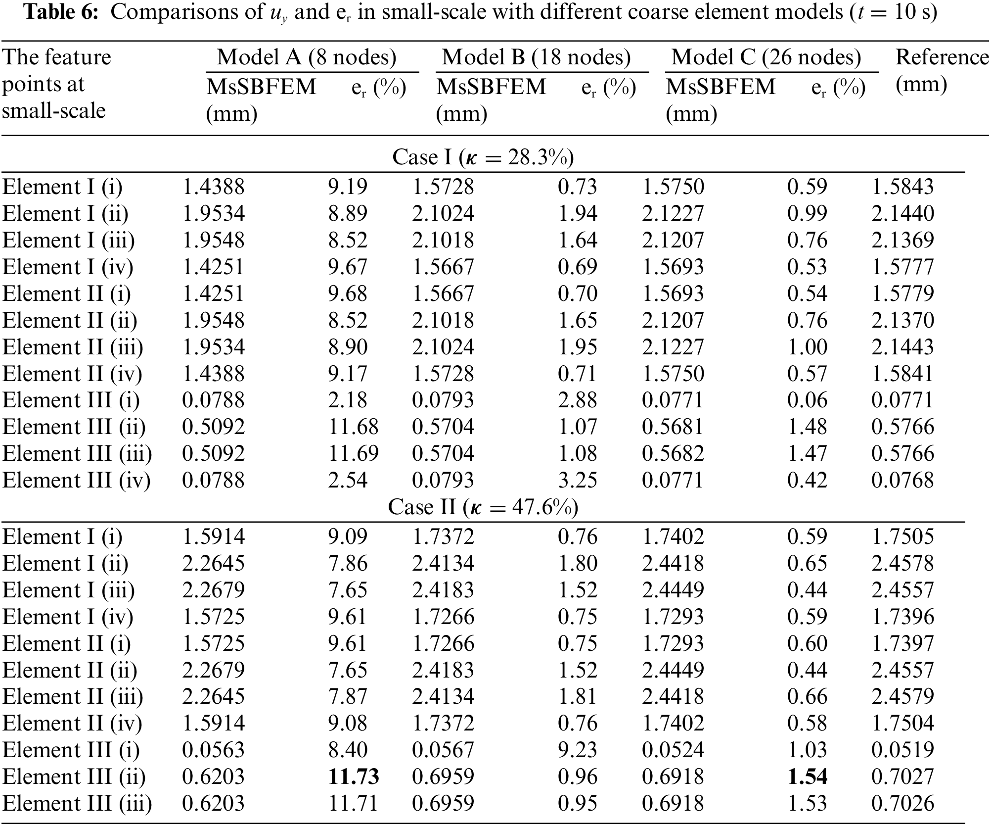
Thirdly, by comparing the computational results for the coarse element Model A (8 nodes), Model B (18 nodes), and Model C (26 nodes) as shown in Fig. 7, Tables 5 and 6 show the result of displacement uy calculated by different models for large feature points and small-scale feature points of coarse elements I–III (see Figs. 6b and 7d) when t = 10 s. These results demonstrate that when the number of coarse nodes increases from 8 to 26, the computational accuracy significantly improves as the maximum error in large-scale decreases from 12.50% to 1.43%. Accordingly, the maximum error in small-scale also decreases from 11.73% to 1.54%. Notably, we increase only the number of coarse nodes here but the octree mesh used in the small-scale is not altered.

4.2 A Cube Domain with Non-Periodic Spherical Inclusions

Consider a heterogeneous cube with the boundary conditions and geometric parameters shown in Fig. 11. The cube contains 27 spherical inclusions of different sizes and the material parameters are shown in Table 7. Accordingly, 27 course elements are used to discretize the cube on large-scale as shown in Fig. 11b. The reference solution is provided using the convergence results of Abaqus with the mesh shown in Fig. 12. The coarse grid in large-scale and the fine grid in small-scale are shown in Figs. 11b and 13, respectively.

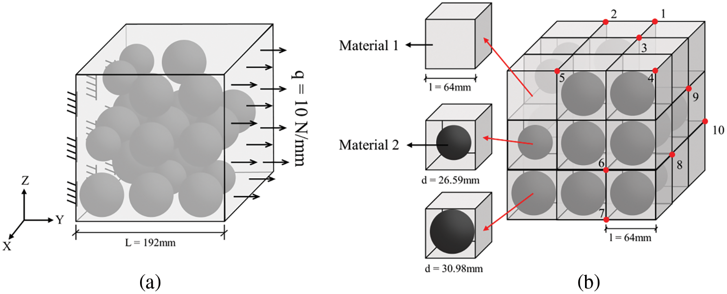
Figure 11: A cube with non-periodic spherical inclusions (a) matrix, inclusions and boundary conditions (b) coarse mesh and the material distribution

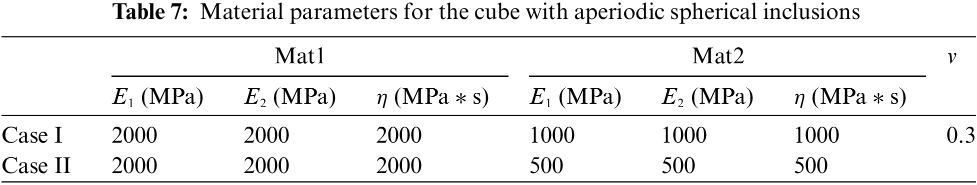
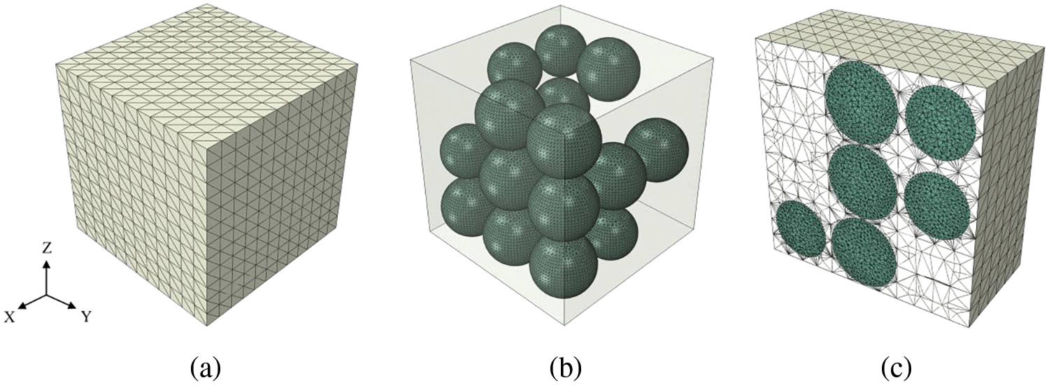
Figure 12: FE mesh in reference solution based on Abaqus (a) outer surface (b) inclusions (c) profile

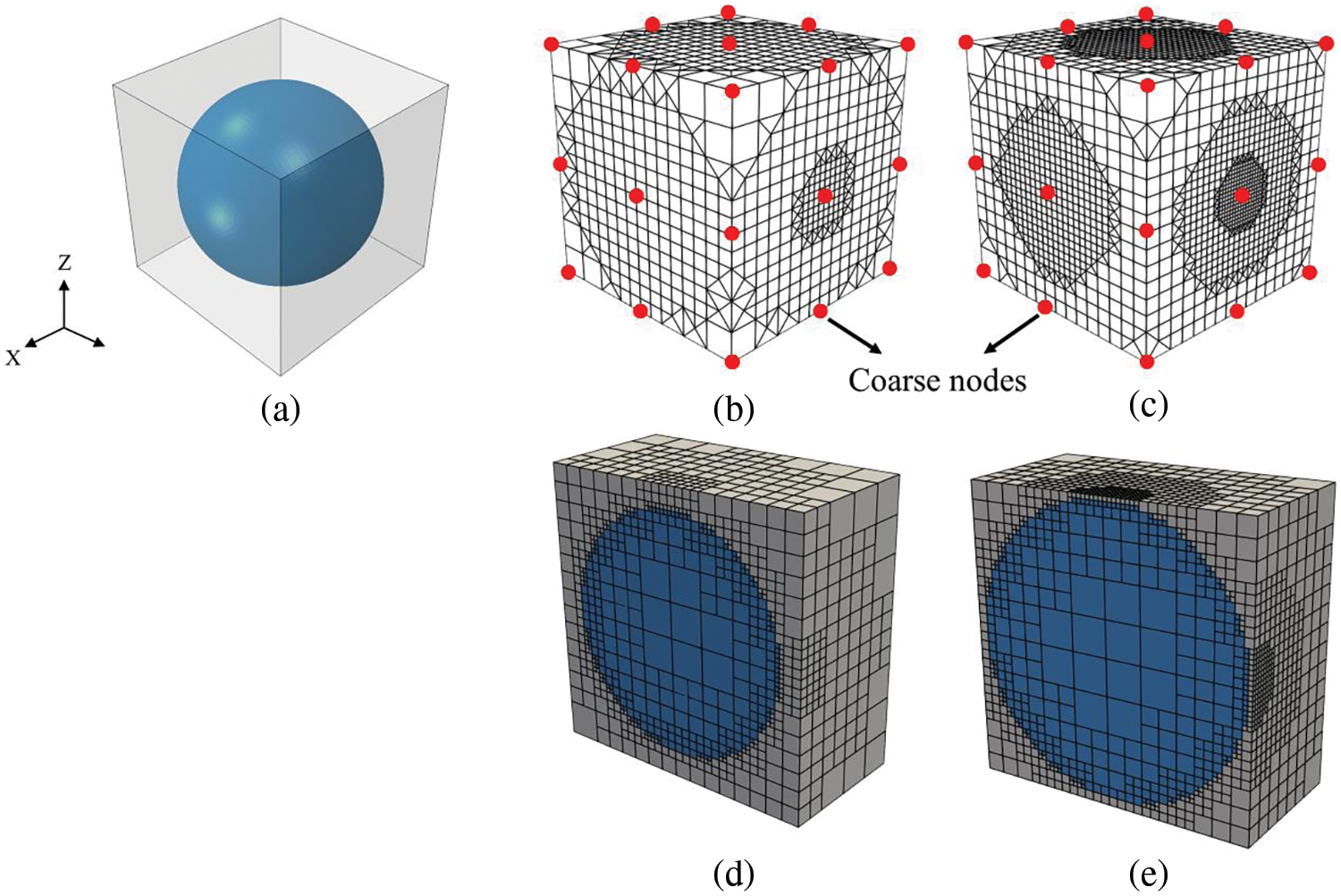
Figure 13: SBFEs with different size of spherical inclusions (a) geometric model (b) inclusion diameter d = 26.59 mm (c) inclusion diameter d = 30.98 mm (d, e) section view of octree mesh

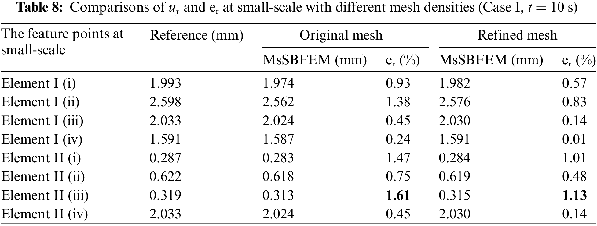
In order to test the influence of quadtree mesh near the interface regions on calculation accuracy, we use the two sizes of quadtree grids shown in Fig. 14 to calculate four small-scale feature points in the coarse elements. Table 8 shows that the maximum relative error is decreased from 1.61% to 1.13% as the minimal size of the elements in small-scale is refined from 2 to 1 mm.

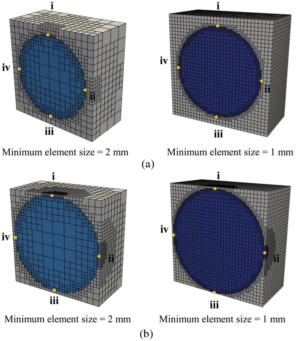
Figure 14: Two different sizes of small-scale grids (a) course element I (b) course element II

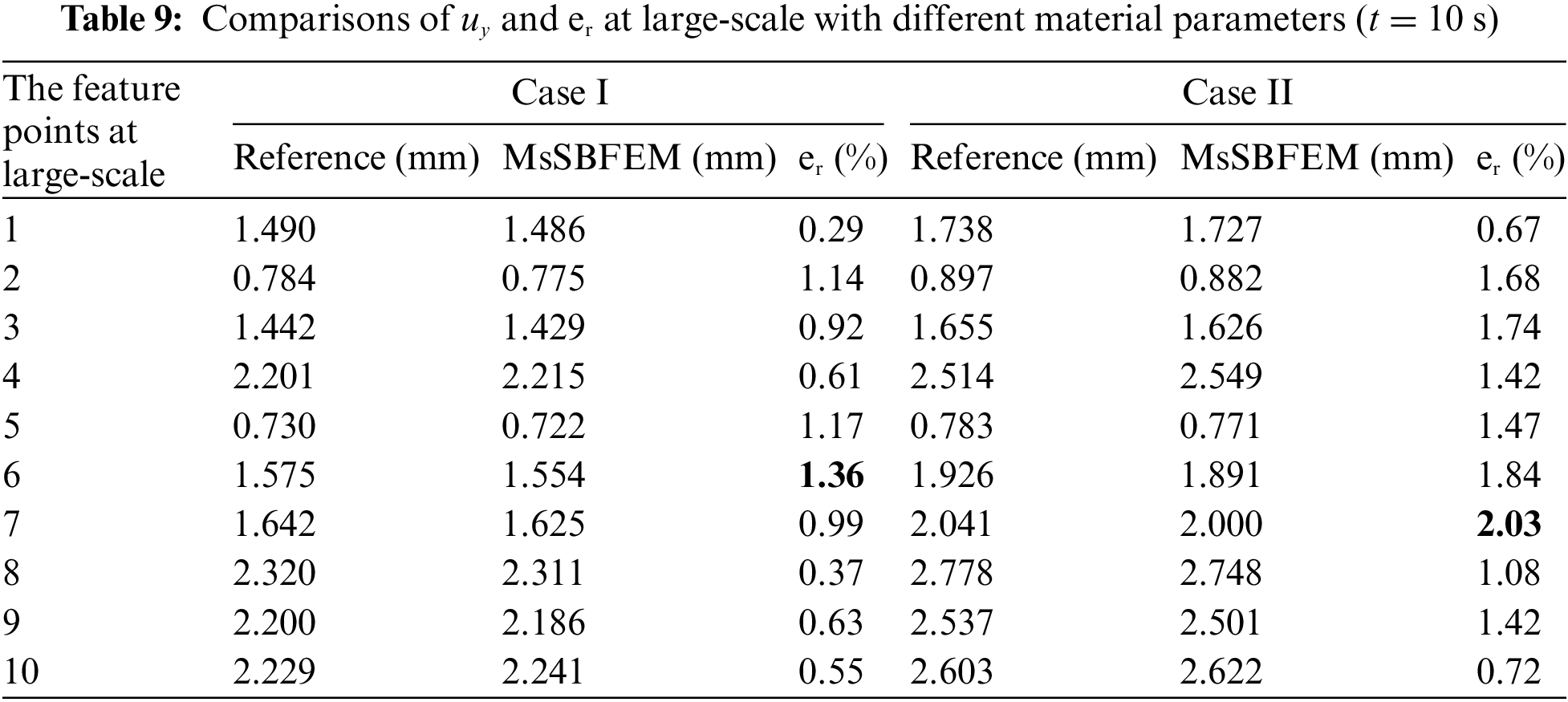
The accuracy of the proposed model in large scale is verified by using the two cases of material parameters (see Table 7). Table 9 shows the displacements at the feature points (shown in Fig. 11b) and the relative error er when the t = 10 s. When the difference in material parameters between the two materials increases, the maximum error of large-scale feature points only increases from 1.36% to 2.03%, showing that the proposed algorithm maintains good accuracy for varying material properties.

To verify the performance of the method in small-scale, we compare the displacement-time curves of several specific points in different coarse elements with two material parameters in Fig. 15. The contour of the displacement field for the entire structure at t = 10 s is illustrated in Fig. 16. Here the coarse element with 26 nodes (Model C) is used. The results show that the proposed method still performs well in computing the displacement values in small-scale feature points and the displacement field in the entire structure with non-periodic inclusions.

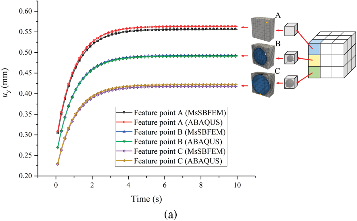
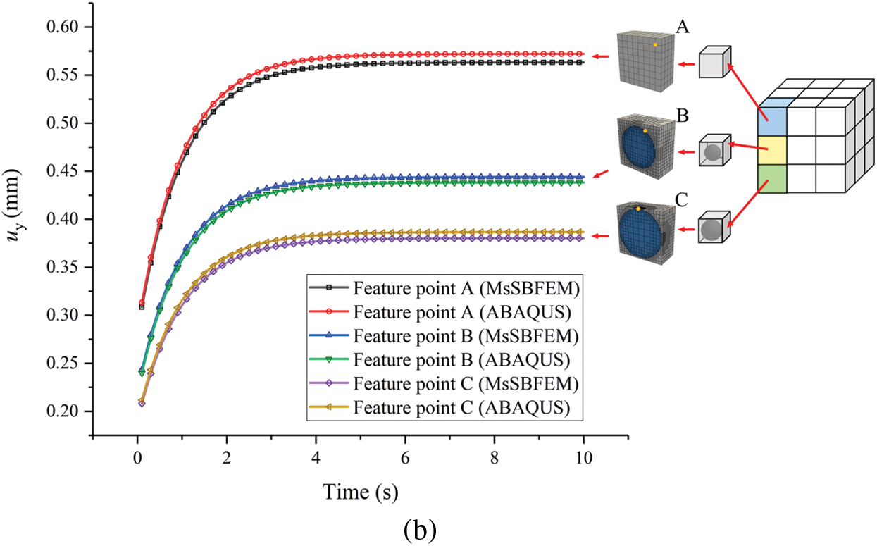
Figure 15: Displacement-time curves of different small-scale feature points (a) material parameters case I (b) material parameters case II

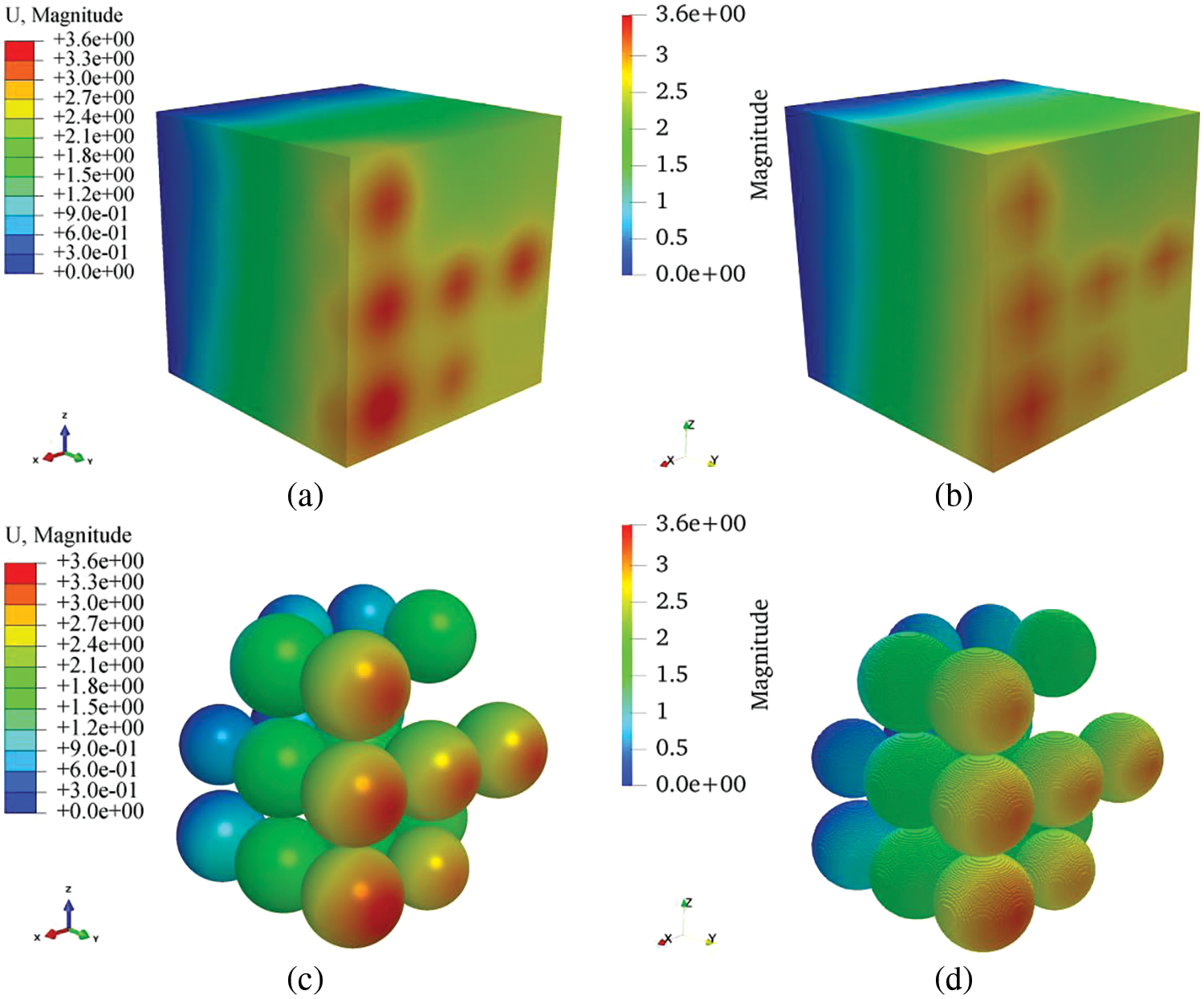
Figure 16: Displacement field cloud map of Case II (t = 10) (a) reference solution for entire structure (b) MsSBFM solution for entire structure (c) reference solution for inclusion displacements (d) MsSBFM solution for inclusions

4.3 A Concrete Beam

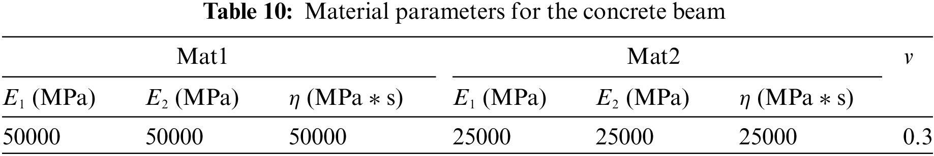
Consider a heterogeneous concrete beam under uniaxial tension with the boundary conditions and geometric parameters shown in Fig. 17. For simplicity, the beam is assumed to have 16 periodic subdomains for simplicity, and the CT images [68–70] of the microstructure of one subdomain are shown in Fig. 18 with the material parameters listed in Table 10. A total of 16 coarse elements are used in large-scale as shown in Fig. 17b.

Figure 17: Image-based mesh generation in small-scale of a concrete beam

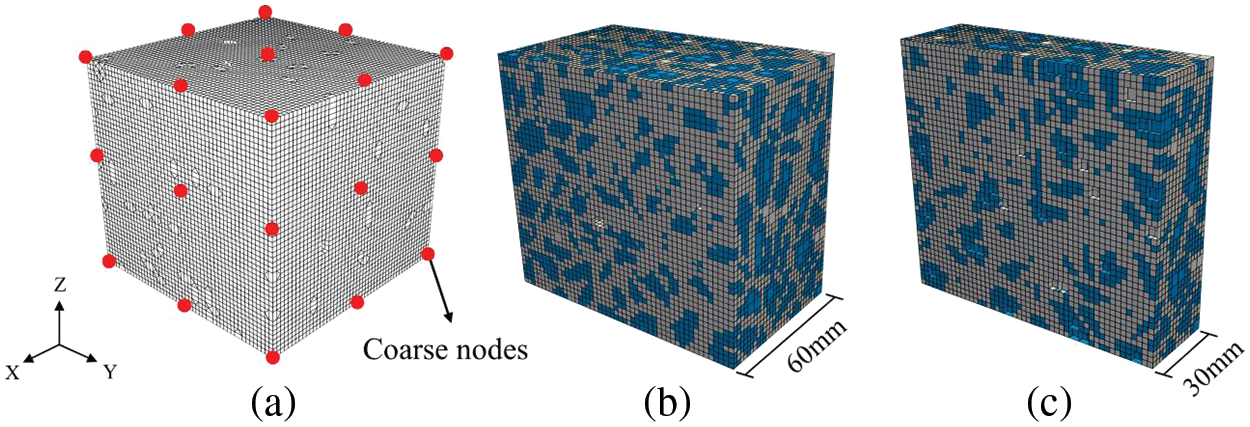
Figure 18: Coarse SBFE and its octree mesh (a) SBFEs for coarse element (b) octree mesh for material 1 (c) octree mesh for material 2

A fine grid in small-scale is shown in Fig. 18. Similar to the previous example in Section 4.1, a total of 26 nodes for each coarse element are used. This means that we use 209 coarse nodes in this example.

Table 11 shows the displacements at feature points in large-scale (shown in Fig. 17) and their relative errors er when the t = 10 s. The reference solution is provided by DNS in commercial software Abaqus with the use of 1885529 nodes as shown in Fig. 19. The average er of the proposed method at feature points is 1.87%, indicating that the proposed method can still obtain a good accuracy when the microstructures are very complex.

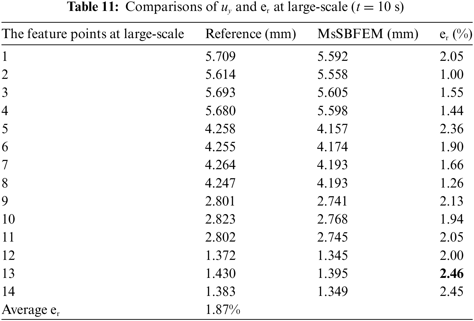
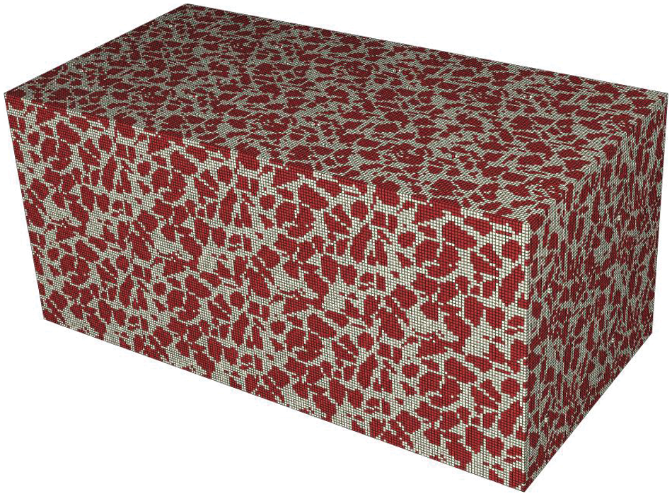
Figure 19: FE mesh in reference solution for DNS by Abaqus (1885529 nodes)

Figs. 20 and 21 show the displacement-time curves of the feature points on different profiles of one specific coarse element and the contour of the displacement field of this coarse element at various times, respectively. As shown in the figure, the results of the proposed model also align well with the reference solution in small-scale.

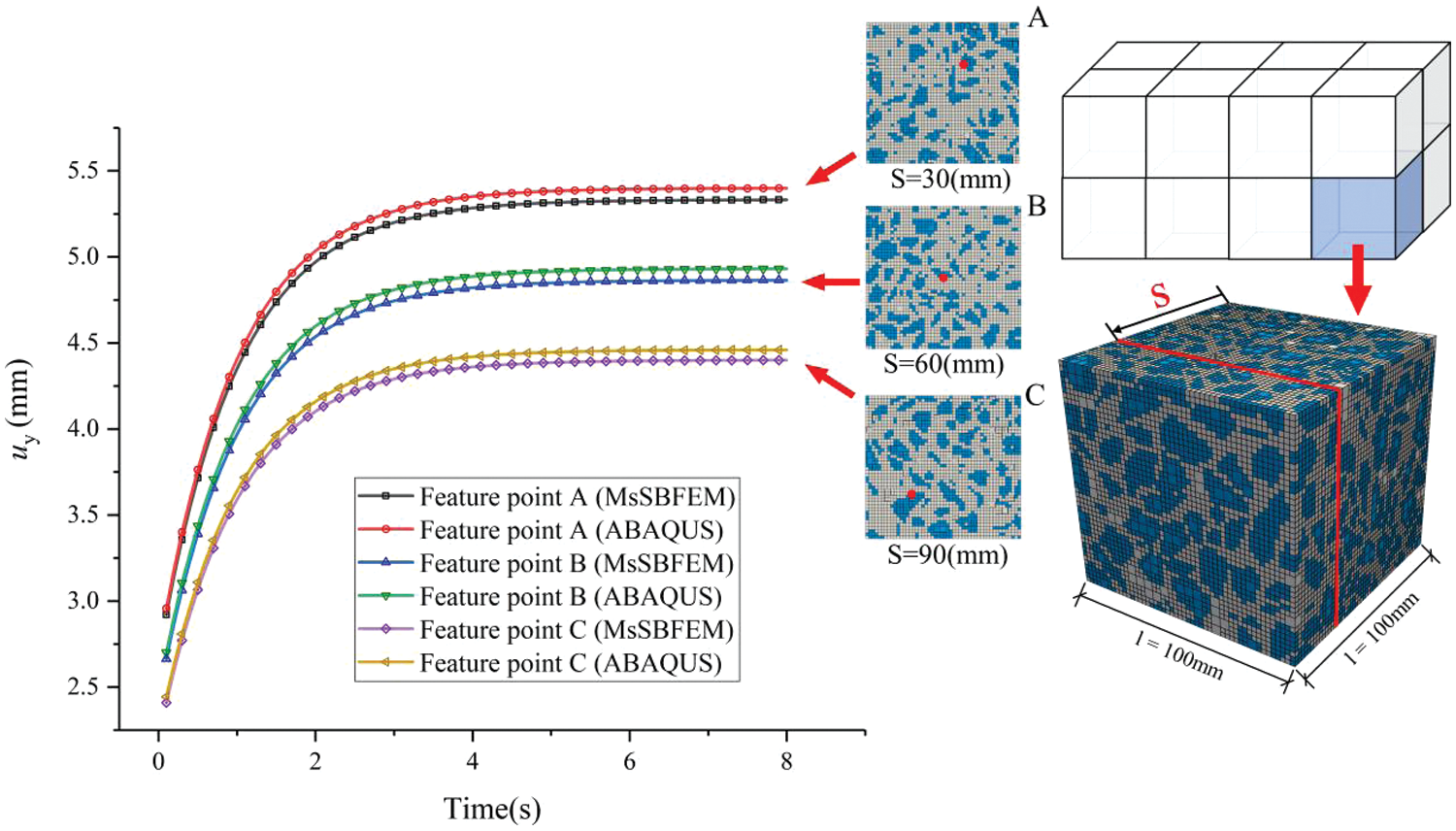
Figure 20: Displacement-time curves of different small-scale feature points in a coarse element

Figure 21: Displacement field cloud maps of feature coarse elements at different time steps (a) FE solution of Abaqus (b) proposed method

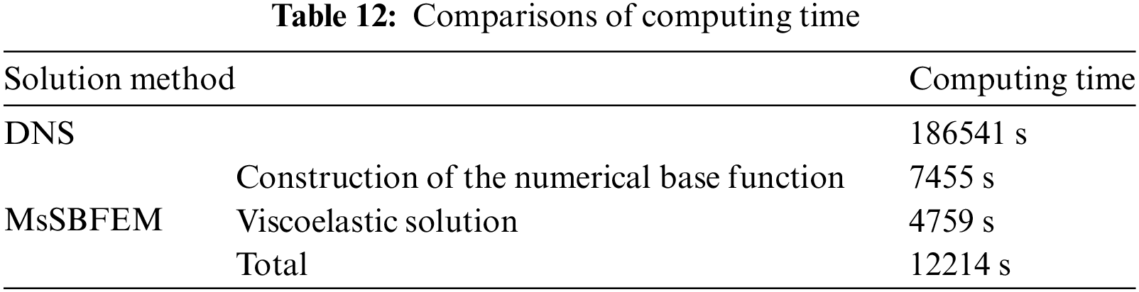
Table 12 shows the comparison of computational efficiency between the DNS and the MsSBFEM, in which Abaqus uses 1885529 nodes and MsSBFEM uses 209 coarse nodes to solve the problem. It is shown that the DNS solution takes 186541 s and MsSBFEM takes 12214 s, the computational efficiency has been improved by 154 times.

5  Conclusions

By integrating the advantages of the MsSBFEM and the temporally piecewise adaptive algorithm, a new numerical algorithm is developed for multiscale analysis of three-dimensional viscoelastic problems of heterogeneous materials by extending the two-dimensional method presented in our previous work. The major merits of this study include

1.    The proposed multiscale method provides an effective tool for handling three-dimensional viscoelastic analysis, that can strongly reproduce realistic situations for heterogeneous viscoelastic analysis, e.g., in the viscoelastic analysis for concrete structures with complex microstructures in Example 3.

2.    The solution scale for three dimensions can be significantly reduced by the proposed multiscale model and the computational accuracy is still satisfactory. For instance, in Example 3, only 209 coarse nodes are used in the proposed method instead of 1885529 nodes in the DNS reference solution, but the average relative error of the proposed method is 1.87%.

3.    Using the octree SBFEM to construct the numerical base functions, the image-based analysis can be conveniently achieved for complex three-dimensional microstructures.

4.    In the time domain, the temporally piecewise adaptive algorithm ensures stable computational accuracy in both large and small scales with different time steps.

5.    Based on the flexibility of the octree SBFEM, nodes can be added on large-scale without changing the mesh on small scale, which can significantly improve the calculation accuracy of the multiscale three-dimensional viscoelastic analysis.

A limitation of this work is that we currently use regular octree meshes in all of the structures; therefore, there could be jagged shapes at the interfaces, producing some errors because the smooth boundaries cannot be exactly described. Although the computational accuracy of the current model is acceptable compared with reference solutions and can also be increased by mesh refinement, a direct cutting mesh method will be further studied in order to better describe material interfaces and increase computational accuracy.

In summary, the proposed method provides an effective new approach for solving three-dimensional multiscale viscoelastic problems. This method can be extended further to solve other three-dimensional time-dependent problems, e.g., the dynamics analysis and the transient heat transfer analysis. Moreover, the extension of the proposed method to nonlinear multiscale analysis is also underway.

Acknowledgement: The authors acknowledge the advices on SBFEM from Prof. Chongmin Song from UNSW and the advices on MsFEM from Prof. Yonggang Zheng from DUT.

Funding Statement: The research leading to this paper was funded by the NSFC Grants (12072063, 11972109), Grant of State Key Laboratory of Structural Analysis for Industrial Equipment (S22403), National Key Research and Development Program of China (2020YFB1708304) and Alexander von Humboldt Foundation (1217594).

Author Contributions: The authors confirm contribution to the paper as follows: study conception and design: Xu Xu, Xiaoteng Wang, Yiqian He, Haitian Yang; data collection: Zhenjun Yang, Xu Xu; analysis and interpretation of results: Xu Xu, Yiqian He; draft manuscript preparation: Xu Xu, Xiaoteng Wang, Yiqan He; draft review: Yiqian He, Zhenjun Yang, Haitian Yang. All authors reviewed the results and approved the final version of the manuscript.

Availability of Data and Materials: The data that support the findings of this study are available from the first and corresponding authors upon reasonable request.

Conflicts of Interest: The authors declare that they have no conflicts of interest to report regarding the present study.

References

1. Wang Y, Artz T, Beel A, Shao XD, Fish J. Computational analyses of flexural behavior for ultrahigh performance fiber reinforced concrete bridge decks. Int J Multiscale Com. 2020;18(4):477–91. doi:10.1615/IntJMultCompEng.v18.i4. [Google Scholar] [CrossRef]

2. Deng L, Fan S, Zhang Y, Huang ZG, Zhou HM, Jiang SF, et al. Multiscale modeling and simulation of polymer blends in injection molding: a review. Polymers. 2021;13(21):3783. doi:10.3390/polym13213783. [Google Scholar] [PubMed] [CrossRef]

3. Sabar H, Berveiller M, Favier V, Berbenni S. A new class of micro-macro models for elastic-viscoplastic heterogeneous materials. Int J Solids Struct. 2002;39(12):3257–76. doi:10.1016/S0020-7683(02)00256-1. [Google Scholar] [CrossRef]

4. Haddad H, Guessasma M, Fortin J. Heat transfer by conduction using DEM-FEM coupling method. Comp Mater Sci. 2014;81:339–47. doi:10.1016/j.commatsci.2013.08.033. [Google Scholar] [CrossRef]

5. Markovic D, Ibrahimbegovic A. On micro-macro interface conditions for micro scale based FEM for inelastic behavior of heterogeneous materials. Comput Method Appl M. 2004;193(48–51):5503–23. [Google Scholar]

6. He Y, Guo J, Yang H, Fu Q. Numerical prediction of effective properties for heterogeneous viscoelastic materials via a temporally recursive adaptive quadtree SBFEM. Finite Elem Anal Des. 2020;177:103426. doi:10.1016/j.finel.2020.103426. [Google Scholar] [CrossRef]

7. Zhang H, Wu J, Fu Z. Extended multiscale finite element method for elasto-plastic analysis of 2D periodic lattice truss materials. Comput Mech. 2010;45:623–35. doi:10.1007/s00466-010-0475-3. [Google Scholar] [CrossRef]

8. Voigt W. Ueber die Beziehung zwischen den beiden Elasticitätsconstanten isotroper Körper. Ann Phys. 1889;274(12):573–87. doi:10.1002/andp.v274:12. [Google Scholar] [CrossRef]

9. Reuß A. Berechnung der fließgrenze von mischkristallen auf grund der plastizitätsbedingung für einkristalle. Zamm-Z Angew Math Me. 1929;9(1):49–58. doi:10.1002/zamm.v9:1. [Google Scholar] [CrossRef]

10. Hashin ZA, Shtrikman S. On some variational principles in anisotropic and nonhomogeneous elasticity. J Mech Phys Solids. 1962;10(4):335–42. doi:10.1016/0022-5096(62)90004-2. [Google Scholar] [CrossRef]

11. Zecevic M, Lebensohn RA. New robust self-consistent homogenization schemes of elasto-viscoplastic polycrystals. Int J Solids Struct. 2020;202:434–53. doi:10.1016/j.ijsolstr.2020.05.032. [Google Scholar] [CrossRef]

12. Wei H, Wang X, Chen C, Jiang K. An adaptive virtual element method for the polymeric self-consistent field theory. Comput Math Appl. 2023;141:242–54. doi:10.1016/j.camwa.2023.01.039. [Google Scholar] [CrossRef]

13. Liu TR, Yang Y, Bacarreza OR, Tang S, Aliabadi M. An extended full field self-consistent cluster analysis framework for woven composite. Int J Solids Struct. 2023;281:112407. doi:10.1016/j.ijsolstr.2023.112407. [Google Scholar] [CrossRef]

14. Mori T, Tanaka K. Average stress in matrix and average elastic energy of materials with misfitting inclusions. Acta Metall. 1973;21(5):571–4. doi:10.1016/0001-6160(73)90064-3. [Google Scholar] [CrossRef]

15. Fedotov A. Mori-Tanaka experimental-analytical model for predicting engineering elastic moduli of composite materials. Compos Part B-Eng. 2022;232:109635. doi:10.1016/j.compositesb.2022.109635. [Google Scholar] [CrossRef]

16. Barral M, Chatzigeorgiou G, Meraghni F, Léon R. Homogenization using modified Mori-Tanaka and TFA framework for elastoplastic-viscoelastic-viscoplastic composites: theory and numerical validation. Int J Plasticity. 2020;127:102632. doi:10.1016/j.ijplas.2019.11.011. [Google Scholar] [CrossRef]

17. Zhang H, Wu JK, Lü J, Fu Z. Extended multiscale finite element method for mechanical analysis of heterogeneous materials. Acta Metall Sin. 2010;26(6):899–920. [Google Scholar]

18. He Z, Pindera MJ. Finite volume-based asymptotic homogenization of periodic materials under in-plane loading. Int J Appl Mech. 2020;87(12):121010. doi:10.1115/1.4048201. [Google Scholar] [CrossRef]

19. He Z, Liu J, Chen Q. Higher-order asymptotic homogenization for piezoelectric composites. Int J Solids Struct. 2023;264:112092. doi:10.1016/j.ijsolstr.2022.112092. [Google Scholar] [CrossRef]

20. Liu P, Liu A, Peng H, Tian L, Liu J, Lu L. Mechanical property profiles of microstructures via asymptotic homogenization. Comput Graphics. 2021;100:106–15. doi:10.1016/j.cag.2021.07.021. [Google Scholar] [CrossRef]

21. Sun W, Fish J, Dhia HB. A variant of the s-version of the finite element method for concurrent multiscale coupling. Int J Multiscale Com. 2018;16(2):187–207. doi:10.1615/IntJMultCompEng.v16.i2. [Google Scholar] [CrossRef]

22. Sun W, Fish J, Ni P. Superposition-based concurrent multiscale approaches for poromechanics. Int J Numer Meth Eng. 2021;122(24):7328–53. doi:10.1002/nme.v122.24. [Google Scholar] [CrossRef]

23. Sun W, Bao S, Zhou J, Ni P. Concurrent multiscale analysis of anti-seepage structures in embankment dam based on the nonlinear Arlequin method. Eng Anal Bound Elem. 2023;149:231–47. doi:10.1016/j.enganabound.2023.01.039. [Google Scholar] [CrossRef]

24. Zhao W, Du C, Jiang S. An adaptive multiscale approach for identifying multiple flaws based on XFEM and a discrete artificial fish swarm algorithm. Comput Method Appl M. 2018;339:341–57. doi:10.1016/j.cma.2018.04.037. [Google Scholar] [CrossRef]

25. Feyel F, Chaboche JL. FE2 multiscale approach for modelling the elastoviscoplastic behaviour of long fibre SiC/Ti composite materials. Comput Method Appl M. 2000;183(3–4):309–30. [Google Scholar]

26. Zhi J, Raju K, Tay TE, Tan VBC. Multiscale analysis of thermal problems in heterogeneous materials with Direct FE2 method. Int J Numer Meth Eng. 2021;122(24):7482–7503. doi:10.1002/nme.v122.24. [Google Scholar] [CrossRef]

27. Tikarrouchine E, Benaarbia A, Chatzigeorgiou G, Meraghni F. Non-linear FE2 multiscale simulation of damage, micro and macroscopic strains in polyamide 66-woven composite structures: analysis and experimental validation. Compos Struct. 2021;255:112926. doi:10.1016/j.compstruct.2020.112926. [Google Scholar] [CrossRef]

28. Jezdan G, Govindjee S, Hackl K. A variational approach to effective models for inelastic systems. Int J Solids Struct. 2024;286:112567. [Google Scholar]

29. Babuška I, Osborn JE. Generalized finite element methods: their performance and their relation to mixed methods. Siam J Numer Anal. 1983;20(3):510–36. doi:10.1137/0720034. [Google Scholar] [CrossRef]

30. Babuška I, Caloz G, Osborn JE. Special finite element methods for a class of second order elliptic problems with rough coefficients. Siam J Numer Anal. 1994;31(4):945–81. doi:10.1137/0731051. [Google Scholar] [CrossRef]

31. Coda H, Sanches R, Paccola R. Alternative multiscale material and structures modeling by the finite-element method. Eng Comput. 2020;38:1–19. [Google Scholar]

32. Zhelnin M, Kostina A, Plekhov O. Variational multiscale finite-element methods for a nonlinear convection-diffusion–reaction equation. J. Appl Mech Tech Phys. 2020;61:1128–39. doi:10.1134/S0021894420070226. [Google Scholar] [CrossRef]

33. Ye C, Dong H, Cui J. Convergence rate of multiscale finite element method for various boundary problems. J Comput Appl Math. 2020;374:112754. doi:10.1016/j.cam.2020.112754. [Google Scholar] [CrossRef]

34. Zhang H, Fu Z, Wu J. Coupling multiscale finite element method for consolidation analysis of heterogeneous saturated porous media. Adv Water Resour. 2009;32(2):268–79. doi:10.1016/j.advwatres.2008.11.002. [Google Scholar] [CrossRef]

35. Zhang H, Liu H, Wu J. A uniform multiscale method for 2D static and dynamic analyses of heterogeneous materials. Int J Numer Meth Eng. 2013;93(7):714–46. doi:10.1002/nme.v93.7. [Google Scholar] [CrossRef]

36. Zhang H, Lu M, Zheng Y, Zhang S. General coupling extended multiscale FEM for elasto-plastic consolidation analysis of heterogeneous saturated porous media. Int J Numer Anal Met. 2015;39(1):63–95. doi:10.1002/nag.v39.1. [Google Scholar] [CrossRef]

37. Zhang S, Yang D, Zhang H, Zheng Y. Coupling extended multiscale finite element method for thermoelastic analysis of heterogeneous multiphase materials. Comput Struct. 2013;121:32–49. doi:10.1016/j.compstruc.2013.03.001. [Google Scholar] [CrossRef]

38. Klimczak M, Cecot W. An adaptive MsFEM for nonperiodic viscoelastic composites. Int J Numer Meth Eng. 2018;114(8):861–81. doi:10.1002/nme.v114.8. [Google Scholar] [CrossRef]

39. Kabel M, Merkert D, Schneider M. Use of composite voxels in FFT-based homogenization. Comput Method Appl M. 2015;294:168–88. doi:10.1016/j.cma.2015.06.003. [Google Scholar] [CrossRef]

40. Song C, Wolf JP. The scaled boundary finite-element method—alias consistent infinitesimal finite-element cell method—for elastodynamics. Comput Method Appl M. 1997;147(3–4):329–55. [Google Scholar]

41. Jiang S, Sun L, Ooi ET, Ghaemian M, Du C. Automatic mesoscopic fracture modelling of concrete based on enriched SBFEM space and quad-tree mesh. Constr Build Mater. 2022;350:128890. doi:10.1016/j.conbuildmat.2022.128890. [Google Scholar] [CrossRef]

42. Ooi ET, Man H, Natarajan S, Song C. Adaptation of quadtree meshes in the scaled boundary finite element method for crack propagation modelling. Eng Fract Mech. 2015;144:101–17. doi:10.1016/j.engfracmech.2015.06.083. [Google Scholar] [CrossRef]

43. Zhang P, Du C, Zhao W, Sun L. Dynamic crack face contact and propagation simulation based on the scaled boundary finite element method. Comput Method Appl M. 2021;385:114044. doi:10.1016/j.cma.2021.114044. [Google Scholar] [CrossRef]

44. Song C. The scaled boundary finite element method in structural dynamics. Int J Numer Meth Eng. 2009;77(8):1139–71. doi:10.1002/nme.v77:8. [Google Scholar] [CrossRef]

45. Dsouza SM, Varghese TM, Ooi ET, Natarajan S, Bordas SP. Treatment of multiple input uncertainties using the scaled boundary finite element method. Appl Math Model. 2021;99:538–54. doi:. [Google Scholar] [CrossRef]

46. Johari A, Heydari A. Reliability analysis of seepage using an applicable procedure based on stochastic scaled boundary finite element method. Eng Anal Bound Elem. 2018;94:44–59. doi:10.1016/j.enganabound.2018.05.015. [Google Scholar] [CrossRef]

47. Khajah T, Liu L, Song C, Gravenkamp H. Shape optimization of acoustic devices using the scaled boundary finite element method. Wave Motion. 2021;104:102732. doi:10.1016/j.wavemoti.2021.102732. [Google Scholar] [CrossRef]

48. Zhang W, Xiao Z, Liu C, Mei Y, Youn SK, Guo X. A scaled boundary finite element based explicit topology optimization approach for three-dimensional structures. Int J Numer Meth Eng. 2020;121(21):4878–4900. doi:10.1002/nme.v121.21. [Google Scholar] [CrossRef]

49. Zhang J, Zhao M, Eisenträger S, Du X, Song C. An asynchronous parallel explicit solver based on scaled boundary finite element method using octree meshes. Comput Method Appl M. 2022;401:115653. doi:10.1016/j.cma.2022.115653. [Google Scholar] [CrossRef]

50. Genes MC. Dynamic analysis of large-scale SSI systems for layered unbounded media via a parallelized coupled finite-element/boundary-element/scaled boundary finite-element model. Eng Anal Bound Elem. 2012;36(5):845–57. doi:10.1016/j.enganabound.2011.11.013. [Google Scholar] [CrossRef]

51. Yu B, Hu P, Saputra AA, Gu Y. The scaled boundary finite element method based on the hybrid quadtree mesh for solving transient heat conduction problems. Appl Math Model. 2021;89:541–71. doi:10.1016/j.apm.2020.07.035. [Google Scholar] [CrossRef]

52. Song C, Ooi ET, Natarajan S. A review of the scaled boundary finite element method for two-dimensional linear elastic fracture mechanics. Eng Fract Mech. 2018;187:45–73. doi:10.1016/j.engfracmech.2017.10.016. [Google Scholar] [CrossRef]

53. Zou D, Chen K, Kong X, Liu J. An enhanced octree polyhedral scaled boundary finite element method and its applications in structure analysis. Eng Anal Bound Elem. 2017;84:87–107. doi:10.1016/j.enganabound.2017.07.007. [Google Scholar] [CrossRef]

54. Wang X, Yang H, He Y. A temporally piecewise adaptive multiscale scaled boundary finite element method to solve two-dimensional heterogeneous viscoelastic problems. Eng Anal Bound Elem. 2023;155:738–53. doi:10.1016/j.enganabound.2023.07.006. [Google Scholar] [CrossRef]

55. Wang X, Yang H, He Y. A multiscale scaled boundary finite element method solving steady-state heat conduction problem with heterogeneous materials. Numer Heat Tr B-Fund. 2023;83(6):345–66. doi:10.1080/10407790.2022.2160850. [Google Scholar] [CrossRef]

56. Zhang J, Eisenträger S, Zhan Y, Saputra A, Song C. Direct point-cloud-based numerical analysis using octree meshes. Comput Struct. 2023;289:107175. doi:10.1016/j.compstruc.2023.107175. [Google Scholar] [CrossRef]

57. Liu L, Zhang J, Song C, He K, Saputra AA, Gao W. Automatic scaled boundary finite element method for three-dimensional elastoplastic analysis. Int J Mech Sci. 2020;171:105374. doi:10.1016/j.ijmecsci.2019.105374. [Google Scholar] [CrossRef]

58. Liu L, Zhang J, Song C, Birk C, Saputra AA, Gao W. Automatic three-dimensional acoustic-structure interaction analysis using the scaled boundary finite element method. J Comput Phys. 2019;395:432–60. doi:10.1016/j.jcp.2019.06.033. [Google Scholar] [CrossRef]

59. Liu Y, Saputra AA, Wang J, Tin-Loi F, Song C. Automatic polyhedral mesh generation and scaled boundary finite element analysis of STL models. Comput Method Appl M. 2017;313:106–32. doi:10.1016/j.cma.2016.09.038. [Google Scholar] [CrossRef]

60. Ya S, Eisenträger S, Song C, Li J. An open-source ABAQUS implementation of the scaled boundary finite element method to study interfacial problems using polyhedral meshes. Comput Method Appl M. 2021;381:113766. doi:10.1016/j.cma.2021.113766. [Google Scholar] [CrossRef]

61. Talebi H, Saputra A, Song C. Stress analysis of 3D complex geometries using the scaled boundary polyhedral finite elements. Comput Mech. 2016;58:697–715. doi:10.1007/s00466-016-1312-0. [Google Scholar] [CrossRef]

62. Zhang J, Natarajan S, Ooi ET, Song C. Adaptive analysis using scaled boundary finite element method in 3D. Comput Method Appl M. 2020;372:113374. doi:10.1016/j.cma.2020.113374. [Google Scholar] [CrossRef]

63. Saputra AA, Eisenträger S, Gravenkamp H, Song C. Three-dimensional image-based numerical homogenisation using octree meshes. Comput Struct. 2020;237:106263. doi:10.1016/j.compstruc.2020.106263. [Google Scholar] [CrossRef]

64. Gravenkamp H, Saputra AA, Eisenträger S. Three-dimensional image-based modeling by combining SBFEM and transfinite element shape functions. Comput Mech. 2020;66(4):911–30. doi:10.1007/s00466-020-01884-4. [Google Scholar] [CrossRef]

65. Wang CS, He YQ, Yang HT. A SBFEM and sensitivity analysis based algorithm for solving inverse viscoelastic problems. Eng Anal Bound Elem. 2019;106:588–98. doi:10.1016/j.enganabound.2019.06.014. [Google Scholar] [CrossRef]

66. He Y, Yang H. Solving viscoelastic problems by combining SBFEM and a temporally piecewise adaptive algorithm. Mech Time-Depend Mat. 2017;21:481–97. doi:10.1007/s11043-017-9338-z. [Google Scholar] [CrossRef]

67. Wang C, Long X, He Y, Yang H, Han X. An adaptive recursive SBFE algorithm for the statistical analysis of stochastic viscoelastic problems. Comput Method Appl M. 2022;395:114878. doi:10.1016/j.cma.2022.114878. [Google Scholar] [CrossRef]

68. Ren W, Yang Z, Sharma R, Zhang C, Withers PJ. Two-dimensional X-ray CT image based meso-scale fracture modelling of concrete. Eng Fract Mech. 2015;133:24–39. doi:10.1016/j.engfracmech.2014.10.016. [Google Scholar] [CrossRef]

69. Yang Z, Ren W, Sharma R, McDonald S, Mostafavi M, Vertyagina Y, et al. In-situ X-ray computed tomography characterisation of 3D fracture evolution and image-based numerical homogenisation of concrete. Cement Concrete Comp. 2017;75:74–83. doi:10.1016/j.cemconcomp.2016.10.001. [Google Scholar] [CrossRef]

70. Huang Y, Yang Z, Ren W, Liu G, Zhang C. 3D meso-scale fracture modelling and validation of concrete based on in-situ X-ray computed tomography images using damage plasticity model. Int J Solids Struct. 2015;67:340–52. [Google Scholar]

Appendix A.

Calculation of Stiffness Matrix of a 3D SBFE

In this paper, the octree grid is used in the small-scale solution, each octree cell is modeled as a scaled boundary cube element, and the cubic centroid O is set as the scaling center. The Cartesian coordinates within the domain (x^,y^,z^) are described by scaling the coordinates on the boundary (x,y,z) along the local radial coordinate ξ, as shown in Fig. A1. For the surface element on the boundary of the cube element, the local coordinate system (η,ζ) is established, based on this coordinate system, the surface element is divided into tetrahedral element and triangular element. For local radial coordinates ξ, at the scaling center ξ=0, on the boundary ξ=1.

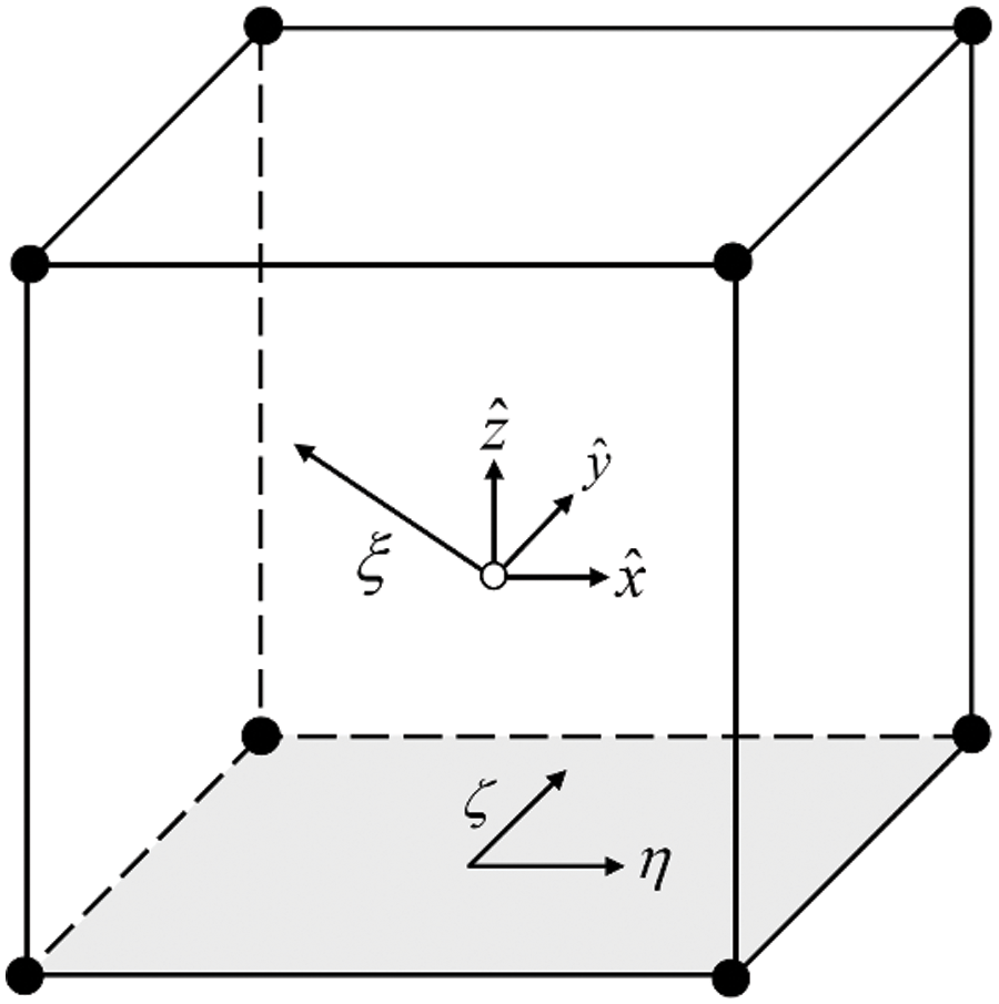
Figure A1: Scaled boundary coordinate system

Assuming that the center of the Cartesian coordinates coincides with the scaling center of scaled boundary coordinates, the transformation relationship between the two coordinate systems is

{x^(ξ,η,ζ)=ξx(η,ζ)=ξN(η,ζ)xy^(ξ,η,ζ)=ξy(η,ζ)=ξN(η,ζ)yz^(ξ,η,ζ)=ξz(η,ζ)=ξN(η,ζ)z(A1)

where N(η,ζ) is the two-dimensional shape function and x,y,z is the node coordinate vector of each surface.

The governing differential equations of 3D elasticity problems in the absence of body forces can be formulated as

LTσ=0(A2)

where σ is the stress vector inside the cube element and L is the linear differential operator, L can be written as

L=b1(η,ζ)∂∂ξ+1ξ[b2(η,ζ)∂∂η+b3(η,ζ)∂∂ζ](A3)

{b1(η,ζ)=1|J|G1b2(η,ζ)=−1|J|(η G1+G2)b3(η,ζ)=−1|J|(ζ G1+G3)(A4)

|J|=x(y,ηz,ζ−z,ηy,ζ)+y(z,ηx,ζ−x,ηz,ζ)+z(x,ηy,ζ−y,ηx,ζ)(A5)

In Eq. (A4), G1,G2 and G3 are the coordinate correlation matrix of the surface element.

The displacement solution of any point in the element can be obtained by radial displacement u(ξ) interpolation.

u(ξ,η,ζ)=Nu(η,ζ)u(ξ)(A6)

where Nu(η,ζ) is the displacement shape function matrix, its specific expression is as follows:

Nu(η,ζ)=[N1(η,ζ)I,N2(η,ζ)I,…,Nn(η,ζ)I](A7)

ε(ξ,η,ζ)=B1u(ξ),ξ+1ξB2u(ξ),ξ(A8)

{B1=b1(η,ζ)Nu(η,ζ)B2=b2(η,ζ)Nu(η,ζ),η+b3(η,ζ)Nu(η,ζ),ζ(A9)

According to the principle of virtual work, the three-dimensional SBFE equation without body forces can be written as

E 0ξ2u(ξ),ξξ+(2E0−E1+E1T)ξu(ξ),ξ+(E1T−E2)u(ξ)=0(A10)

The coefficient matrix is as follows:

{E0=∫−1+1∫−1+1B1TCB1|J|dηdζE1=∫−1+1∫−1+1B2TCB1|J|dηdζE2=∫−1+1∫−1+1B2TCB2|J|dηdζ(A11)

where C is the 6×6 elasticity matrix for three-dimensional problems. The internal node forces on each surface element can be written as

q(ξ)=ξ(E0ξu(ξ),ξ+E1Tu(ξ))(A12)

Transforming Eqs. (A10) and (A12) into a system of first-order ordinary differential equations

ξ{ξ0.5u(ξ)ξ−0.5q(ξ)},ξ=−Z{ξ0.5u(ξ)ξ−0.5q(ξ)}(A13)

where Z is the Hamiltonian matrix, it can be expressed as

Z=[E0−1E1T−0.5I−E0−1−E2+E1E0−1E1T−(E1E0−1−0.5I)](A14)

The matrix Z is decomposed using a Schur decomposition with block diagonalization

ZV=VS(A15)

where S and V are the real Schur form matrix and the transformation matrix, respectively. Divide the matrices S and V into submatrices of the same size, as shown in following equation:

S=[S1100S22](A16a)

V=[V11V12V21V22](A16b)

All the eigenvalues of submatrix S11 have negative real parts which corresponds to the solution of a bounded domain. Therefore, the general solutions for the displacements and internal nodal forces of the bounded domain are

u(ξ)=V11ξ−S11−0.5Ic(A17a)

q(ξ)=V21ξ−S11+0.5Ic(A17b)

K=V21V11−1(A18)