Multi-Material Topology Optimization of 2D Structures Using Convolutional Neural Networks

1  Introduction

Topology optimization, as an effective method for structural design, has garnered significant attention and application. The fundamental principle of topology optimization is to generate an optimized structure by distributing materials within a design domain, considering given loads and constraints. Over the years, various topology optimization methods have been proposed and developed, including Homogenization Design Method (HDM) [1,2], Solid Isotropic Material with Penalization (SIMP) method [3–5], Level-Set Method (LSM) [6,7], Evolutionary Structural Optimization (ESO) method [8], Moving Morphable Component (MMC) method [9,10], phase field method [11] and so on. These methods predominantly rely on gradient algorithms and iterative optimization, necessitating finite element analysis (FEA) at each iteration. With the rapid advancement of additive manufacturing (AM) technology, the manufacturing challenges associated with complex structures designed through topology optimization have significantly diminished. Consequently, topology optimization has gained further traction, leading to the rapid development of research in three-dimensional design [12,13], multi-material design [14,15], multiscale design [16–18], and others [19].

In order to achieve improved structural performance or cost-effectiveness, researchers have long focused on the study of multi-material topology optimization. MMTO has primarily been developed based on binary topology optimization methods. Consequently, according to the classification of several traditional topology optimization methods, the multi-material topology optimization work that has been carried out mainly includes: homogenization method [20–22], SIMP method [23–25], level-set method [26–30], ESO method [31,32], and others [33–35]. One common challenge in MMTO is the increase in the number of design variables as the number of materials increases. Additionally, the inclusion of more discrete elements in finite element analysis further amplifies the number of design variables. Consequently, MMTO encounters significant computational resource requirements when dealing with large-scale computational objects. The necessity for high-performance computing resources and the substantial time requirements remain major challenges for the widespread implementation of MMTO at a large scale.

In recent years, the rapid advancements in computer hardware technology and artificial intelligence (AI), particularly in the field of deep learning using neural networks, have led to their widespread adoption in various traditional domains. In parallel, researchers have explored the integration of topology optimization with neural networks to enhance and optimize structural design. Among the various research directions, the data-driven topology optimization (DDTO) method, as an accelerated solution process, is one of the most important research directions. The primary objective of DDTO is to alleviate the computational burden and conserve computing resources during the analysis and optimization stages. Its core concept revolves around leveraging neural networks, known for their excellent fitting capabilities, as function approximators. Specifically, the neural network learns the inherent rule from existing data samples, enabling it to swiftly solve new problems. Researchers often refer to the trained neural network as a “surrogate model”. Within topology optimization, this surrogate model can directly predict or generate the optimal structure given specific design conditions, effectively replacing the entire topology optimization process and enabling rapid solution generation without the need for iterations. For instance, Zhang et al. [36] developed a convolutional neural network model which identified the optimization structure without any iteration. Abueidda et al. [37] applied ResUnet [38] to build a data-driven surrogate model that can quickly predict the two-dimensional nonlinear structure topology optimization without any iteration. Of course, there is a lot of related works which will be detailed in Section 2.1. By substituting the neural network model for the entire topology optimization process, the optimized structure can be rapidly obtained, significantly reducing the time required and accelerating the design process. Multi-material topology optimization has always been computationally complex, slow in convergence, and computing resource-intensive. Therefore, the development and application of deep learning technology offer an effective approach to enhance and optimize MMTO. At present, most studies on the combination of DL and TO are limited to the optimization of single-material (binary) structures, and few studies on the multi-material design [14]. Whether the MMTO method based on deep learning can develop a novel method for fast solution and explore the factors affecting the modeling needs further research.

In this study, we propose a novel framework for accelerating the MMTO using deep learning. Our approach is based on a data-driven approach that utilizes convolutional neural networks to build a surrogate model to solve a multi-material topologies. Here, a novel coding method combining MMTO and neural network is proposed. The coding method enables the creation of a surrogate model that can rapidly generate multi-material topologies without the need for iterations. To train the neural network, the phase field method is adopted to generate a series of MMTO datasets. The input and output of our network are a multi-channel matrix, with each channel of the input representing a different initial condition and each output channel representing a distribution of a material. The experimental results demonstrate the multi-material topology obtained by the proposed coding method has clear material boundaries and high prediction accuracy. In addition, in order to choose the appropriate surrogate model mapping between regression and classification tasks, the proposed framework can identify higher-precision surrogate models within the same dataset. Lastly, through a series of experiments, we investigate the key factors that influence the construction of surrogate models for MMTO. The obtained results will provide valuable guidance for future research in the field of multi-material topology optimization, particularly in the context of deep learning.

The remainder of the paper is as follows. Section 2 reviews the related literature and multiphase topology optimization. In Section 3, we describe the proposed approach in detail, including the multiphase topology optimization framework using deep learning, data generation, network architecture, loss function, and evaluating metrics. In Section 4, we elaborate the experimental results and discussion. Finally, Section 5 concludes the paper and discusses the future works.

2  Overview of Related Works

In this section, we will focus on deep learning for topology optimization and multiphase topology optimization.

2.1 Deep Learning for Topology Optimization

In recent years, there has been a surge in research efforts aimed at leveraging deep learning techniques to reduce the computational burden of topology optimization and accelerate the design process. Li et al. [39] proposed a non-iterative topology optimization method that utilizes deep learning for the design of conductive heat transfer structures. The network model takes a set of matrices representing the boundary conditions as input and generates the optimized structure as output. The topology optimizer can provide accurate estimation of conductive heat transfer topology in negligible time. In subsequent work [40,41], some changes occurred in the form of model inputs which may include initial stress or displacement field. Lei et al. [42] proposed a data-driven real-time topology optimization paradigm under a moving morphable component-based framework. This method not only reduces the dimension of parameter space but also improves the efficiency of optimization process. Yu et al. [43] and Nakamura et al. [44] utilized a CNN model trained on a large number of samples to predict final optimization structures directly, without the need for iteration. Then, Ates et al. [45] proposed the method though introducing a two-stage convolutional encoder and decoder network. Their approach can improve the prediction performance and reliability of network models relative the single network. Xiang et al. [13] proposed a deep CNN for 3D structural topology optimization, which can predict a near-optimal structure without any iterative scheme. The common characteristic among these studies is that the optimal structure can be obtained through the neural network model without the entire solving process. This significantly accelerates the design process. However, there may be some limitations, such as the occurrence of disconnection phenomena in the output structures and the limited applicability of the obtained CNN models. While these approaches have greatly improved the speed of the optimization process, they may have some limitations.

Compared with replacing the whole TO process directly with neural networks, there are also some works that use neural networks to replace the partial process in topology optimization, such as finite element analysis and so on. The methods and strategies used in these works show a diversified development trend. Several works [46–50] have used neural networks to replace or reduce finite element analysis. What these approaches have in common is training a neural network model to replace complex calculations, and then reducing the cost of the calculations. In addition, Sosnovik et al. [51] used neural networks to map the intermediate structure in the iterative process directly to the final optimized structure. This method reduces the number of iterations and improves the efficiency of the optimization process. Similarly, Banga et al. [12] applied the 3D convolutional neural network to accelerate 3D topology optimization. In this method, the intermediate results of the traditional method ware used as the input of the neural network, which can reduce the computational cost. Similar to the above two works [12,51], the method proposed by [52] divides the structure image into overlapping sub-modules. The sub-modules are then mapped to optimized sub-structures using the model and the complete structure is obtained by integrating these sub-structures. Samaniego et al. [53] mentioned the idea of using deep neural networks as a function fitter to approximate the solution of partial differential equations (PDEs), which has made important advances in efficiency. Yan et al. [40] used the initial principal stress matrix of the structure as the input variable of the model, and can obtain the prediction topologies with higher accuracy on the basis of fewer samples. Compared with the traditional TO method, the proposed method can get similar results in real time without repeated iteration. Wang et al. [54] utilized neural networks to build a mapping network of low-resolution structures to high-resolution structures. Then, the low-resolution structure generated by SIMP method is combined with the neural network to quickly obtain the high-resolution structure. By utilizing neural networks to replace certain steps of the topology optimization process, this approach simplifies the overall process and reduces computational time. Generally, this method still relies on a traditional iterative process to support the generation of the final output structure, which does require a certain amount of time. Nevertheless, the performance of the obtained structure is comparable to that achieved by traditional methods.

To address the computational challenges associated with generating datasets, neural network models combined with generative adversarial network (GAN) [55] and CNN are employed to actively generate structures. This approach aims to reduce computational costs and facilitate diverse design exploration [56–61]. In addition, some researches [14,62–66] applied neural network as an optimizer to carry out TO design, which is called neural reparameterization design. The essence of reparameterization design is to use the ability of neural network to automatically update parameters as an optimizer, which does not require datasets and requires iteration similar to traditional TO methods. The purpose of reparameterization is to represent the structure with fewer design variables, thereby reducing the computational load of the optimization process. We mainly focus on the application of neural network building surrogate models in topology optimization, and other characteristic methods will not be described here. Readers can also refer to the review articles [67,68], which provide a comprehensive summary and introduction to the use of deep learning in TO.

In summary of the above work, we find that there is less research work on deep learning to accelerate MMTO design. There may be the following reasons for the lack of relevant studies. First, the generation and processing of datasets for MMTO are relatively complicated, so it is a challenging research to choose the method to generate high-quality datasets. Second, the effective combination of MMTO and neural network is another difficulty. What kind of combination method can fully consider the volume constraints of the multi-material, and output the multi-material topologies with clear material boundaries. Third, the mapping modeling method also needs to be further studied, which is different from single-material topology that uses a matrix of structure size as the output. The multi-material topology can be represented by multiple matrices where each matrix represents a material, or it can be represented by a matrix with different values representing different materials. At the same time, the characteristics of regression task and classification task for mapping methods should be studied, and the mapping method more suitable for MMTO should be explored. To this end, we will conduct a specific study on the above problems, and introduce several evaluating metrics to evaluate the performance of neural networks for MMTO. Finally, the guidelines for constructing high-precision surrogate models of MMTO are provided through extensive comparative analysis.

2.2 Multiphase Topology Optimization

Compared with the binary phase topology optimization problem, the multiphase topology optimization problem is more complicated and more difficult to calculate by algorithm. For example, in the calculation of multiphase topology optimization problems, the most important aspect is the representation of the material property tensor as a function of physical properties and local volume fractions of individual phases. Here, we will focus on the multiphase topology optimization method proposed by [25,69]. In this section, the statement of a typical multiphase topology optimization problem will be presented.

Fig. 1a describes the general topology optimization of statically linear elastic structures under single load. The design domain of topology optimization problems is denoted by Ω. The design domain Ω⊆Rd(d=1,2,3) is defined as an open set corresponding to the d-dimension. As shown in the Fig. 1a, the design domain is mainly composed of linear isotropic elastic materials, fixed domains and void materials with near zero Young’s modulus. The external body force f and the boundary traction force t will obtain a displacement field u. Here, the solution of a linear elastic system can be expressed as:

{−divσ(u)=fin Ωu=u0on Γ1σ(u)⋅n=0on Γ2σ(u)⋅n=ton Γ3(1)

where σ represents the stress tensor, u0 represents the prescribed displacement on the Dirichlet boundary condition Γ1 [1,25], n represents the outward normal to the boundary, Γ2 represents the Neumann boundary condition. t represents the traction portion of the structure with the environment through the boundary traction condition Γ3. Here, the whole boundary condition consists of three parts: Γ=∂Ω=Γ1∪Γ2∪Γ3. In addition, the strain tensor ε at any point x∈Ω is given in the usual form as:

ε(u)=12(∇u+∇uT)(2)

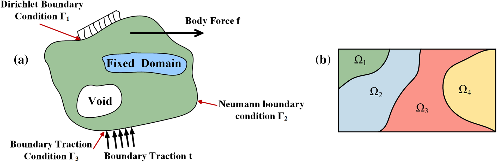
Figure 1: Schematic representation: (a) the topology optimization problem of statically linear elastic structures under single load, (b) the design domain Ω composed of p = 4 material phases

The stress tensor σ can be calculated by the following expression:

σ(u)=Eε(u)(3)

where E represents the elasticity tensor.

In this paper, we consider using p different types of material phases whose material density at a given location x is expressed as an ordered parameter field α(x)=[α1,α2,…,αp]T. The goal of the multimaterial topology optimization problem is to find the optimal distribution of p number of distinct materials inside Ω. For each αi, there will be the following point-wise bound constraints:

0⩽αi⩽1,i=1,…,p(4)

Here, the inequalities are understood componentwise. Since the desired design does not allow gap and overlap, the sum of volume fractions at each point should be equal to one unity. The physical relationship can be expressed as:

∑i=1pαi=1(5)

In many topology optimization problems, there is usually a global volume constraint on the total volume of each material inside Ω.

∫Ωαidx=Vi|Ω|,i=1,…,p(6)

∑i=1pVi=1,0⩽Vi⩽1(7)

Ωi∩Ωj=∅,i≠j(8)

If the volume fraction field of one material is removed, the above problem becomes the problem of solving p−1 unknown topology indicator fields. This way often occurs in binary phase topology optimization problems.

In addition, the material properties of each region are determined by the corresponding material phase. The elasticity tensor at a given location x is given by E(x)=E(α(x)). Here, referring to the principle of SIMP method, the material interpolation operator using linear interpolation [69] can be expressed as:

E(α)=∑i=1pαiqEi(9)

where Ei represent the constant elasticity tensor corresponding to phase i-th. As discussed by [35], one of the main features of penalization schemes for multi-material TO problems is to ensure that unique material phases exist at each point in the design domain. Therefore, the penalization schemes designed here can effectively prevent overlap between material phases. In addition, as mentioned by [70], the interpolation of elastic tensors based on Eq. (9) is inherently unreasonable as it can lead to non-realistic physical data. Following their recommendations, a rational interpolation scheme involves computing the Hashin-Shtrikman lower and upper bounds for each physical property. Subsequently, the interpolated elastic tensor is calculated by replacing its components with the corresponding average Hashin-Shtrikman bounds. As highlighted by [71], in practical computational processes, finding the Hashin-Shtrikman bounds for an arbitrary number of phases is not always straightforward. Additionally, under certain conditions, the volume fractions and physical properties of the original phases can reach the Hashin-Shtrikman bounds. Therefore, this study relies solely on the aforementioned relationships to construct the model problem and cautions readers to exercise extreme caution when utilizing this relationship.

Here, for the basic minimum compliance problem in structural optimization, the objective function is as follows:

minimizeC(u,α)=∫Ωf⋅udΩ+∫Γ3t⋅udΓsubject to: ∑i=1pαi=1∫Ωαidx=Vi|Ω|,i=1,…,p0⩽αi⩽1,i=1,…,p12∫Ωεij(u):Eijkl(α)εkl(v)dΩ=∫Ωf⋅vdΩ+∫Γ3t⋅vdΓ,for all v∈U(10)

where “:” represents the second-order tensor operator and v represents the virtual displacement in the displacement fields within the kinematically admissible range. Here, the gradient of the objective function can simply be calculated using classical adjoint approach.

3  Detailed Approach

3.1 The Multiphase Topology Optimization Framework Using Deep Learning

The calculation principle of multiphase topology optimization follows a similar approach to binary phase topology optimization. The solution process involves iterative calculations using the finite element method, which can be computationally demanding, particularly for complex multiphase design problems. In Fig. 2, we illustrate the solution process for multiphase topology optimization, which includes initial design variables, update variables, finite element solution, sensitivity analysis, and sensitivity filtering. To address the challenges posed by the iterative nature of the traditional approach, our main objective is to develop a deep neural network as a surrogate model. This surrogate model aims to generate multiphase optimization structures in a non-iterative manner. Fig. 2 presents the proposed deep learning framework designed for multiphase topology optimization. This framework encompasses three key processes:

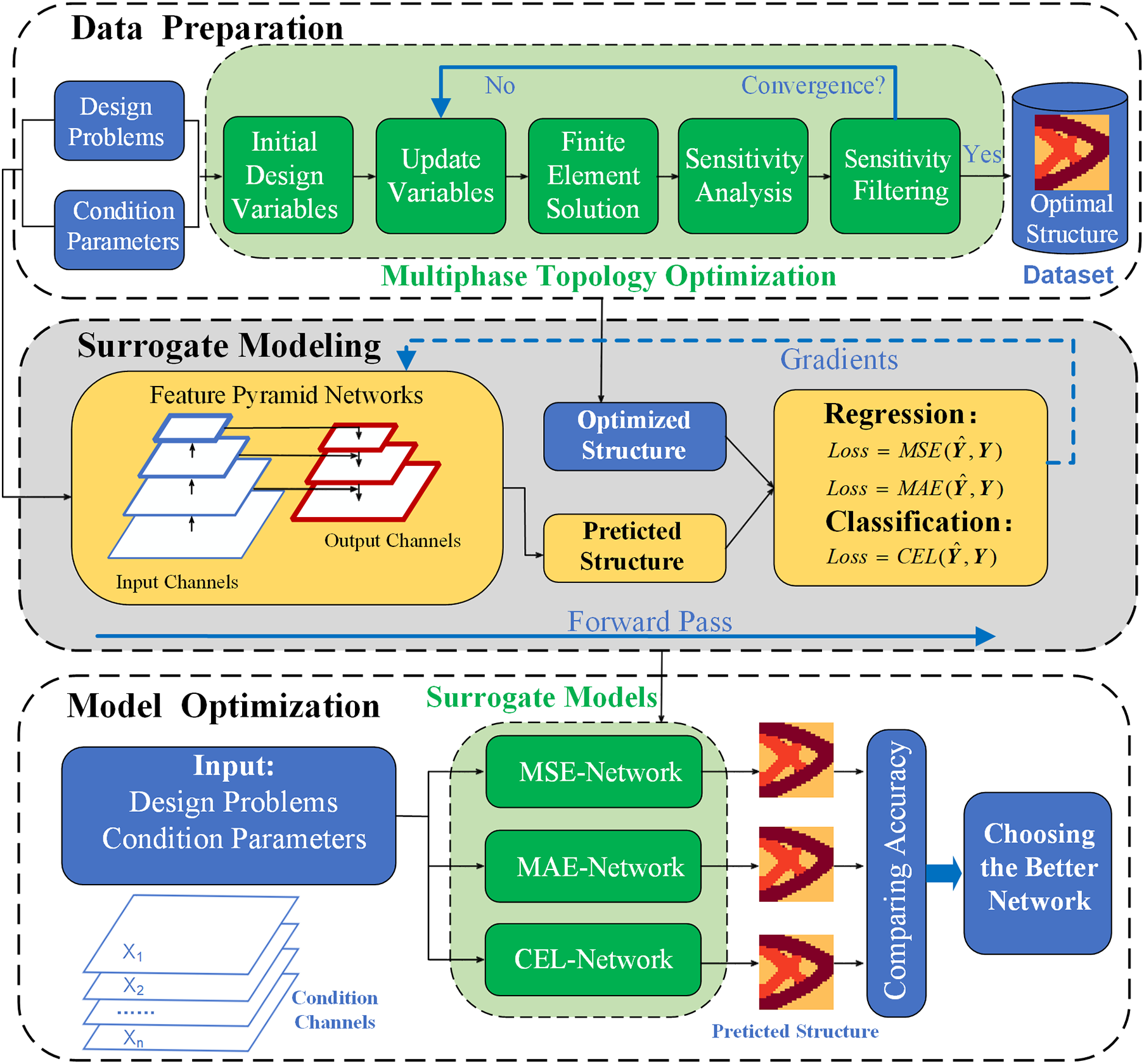
Figure 2: Flowchart showing the framework of multiphase topology optimization using deep learning

Data preparation. We employ three classical topology optimization problems to generate diverse datasets of varying scales in this party. Each data sample in the dataset consists of a multi-channel matrix generated from the input parameters and the corresponding optimized structure. Different datasets are generated by changing the topology optimization problem, the design domain size, the number of material category, and the material properties. To ensure a uniform distribution of the sample design space, we generate the dataset through random sampling. Subsequently, these datasets are utilized as both training and testing data for the surrogate model.

Surrogate modeling. The multi-channel matrix represents the input, while the optimized structure serves as the label for the mapping modeling task. In this study, we employ the feature pyramid network (FPN) to learn the inherent laws within each dataset and utilize it as the surrogate model. It is important to note that the mapping modeling can be viewed as either an image-to-image regression task or a classification task, and the choice of the loss function is crucial in distinguishing between these two tasks. The surrogate modeling process involves optimizing the weight parameters of the neural network, with the objective of minimizing the selected loss function. For regression tasks, the mean square error (MSE) and mean absolute error (MAE) are commonly employed as loss functions. On the other hand, the cross-entropy loss (CEL) function is typically used as the loss function for classification tasks. By selecting different loss functions, we can obtain different surrogate models.

Model optimization. After constructing various surrogate models, the accuracy of surrogate models is evaluated by solving multiple multiphase topology optimization problems using new samples. Subsequently, the surrogate model exhibiting the highest accuracy is chosen as the preferred model for solving similar multiphase topology optimization problems. Furthermore, the test results from the next stage can serve as a reference for determining the hyperparameters of the surrogate modeling process.

3.2 Data Generation

This section details the data combinations for the topology optimization problems mentioned in Section 4. As shown in Fig. 3, we prepare three types of datasets, which are generated by three classical topology optimization problems (cantilever beams, Messerschmitt Bölkow Blohm (MBB) beams and Michell beams). Because the methods of generating data by using several different TO problems are similar, this paper mainly introduces the generation of multi-material topology optimization data by using cantilever beam as the representative. The difficulty in generating data is how to represent the volume constraints of each material and clearly represent the multi-material structural topology. Therefore, we present a multi-material coding approach to better combine neural networks to build surrogate models. In this study, the materials are linear elastic materials which conform to Hooke’s law, and are represented as isotropic. Each topology optimization problem is used to generate multiple datasets of different sizes. Each dataset consists of multiple topology optimization samples, each of which includes information such as boundary conditions, loading conditions, volume fraction of each material, and optimized structural topology (material distribution).

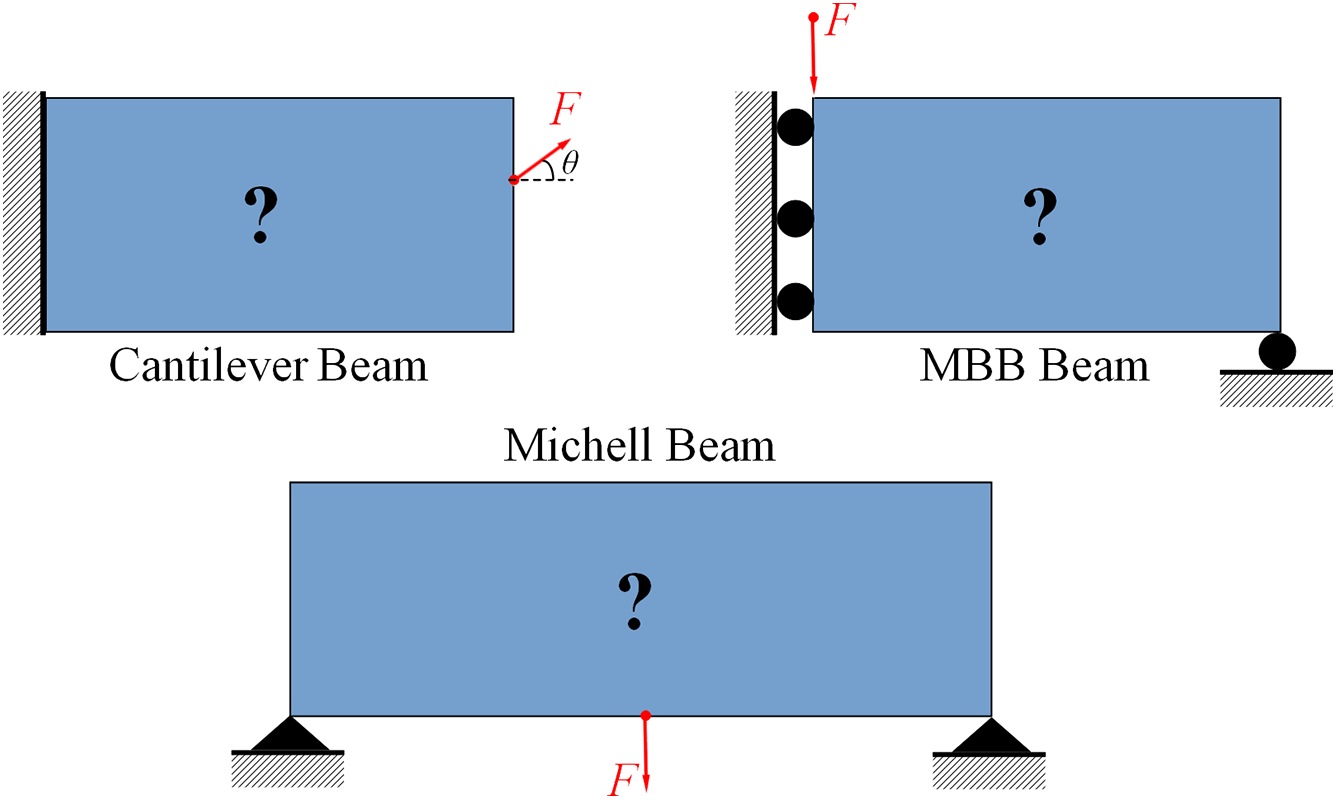
Figure 3: Geometries and boundary conditions corresponding to different topology optimization problems

As illustrated in Fig. 4, the optimized cantilever structure of three-phase material (denoated as M1, M2, M3) is utilized, incorporating multiple channels for the input and output of the neural network. The design domain employs a nx×ny=32×32 finite element mesh to discrete the linear elastic structure. The boundary conditions of the cantilever are fixed to the left. Four-node element is used in finite element analysis. The Young’s modulus (E) values for all phases are set as [9, 3, 1e-9], and the Poisson’s ratio is set to 0.3 for all phases. The applied force on the structure is F=1. The filter radius (Rmin) is set to 2, while the penalty parameter q is set to 3. The parameters of samples primarily include the loading angle, loading position, and volume fraction. The random conditions for these parameters are subject to a uniform distribution, as described below:

•   Volume fraction: in accordance with Eq. (7)

•   Loading position: the node selected from the nodes set at the right-hand side of the design domain

•   Loading direction: [0, 360°]

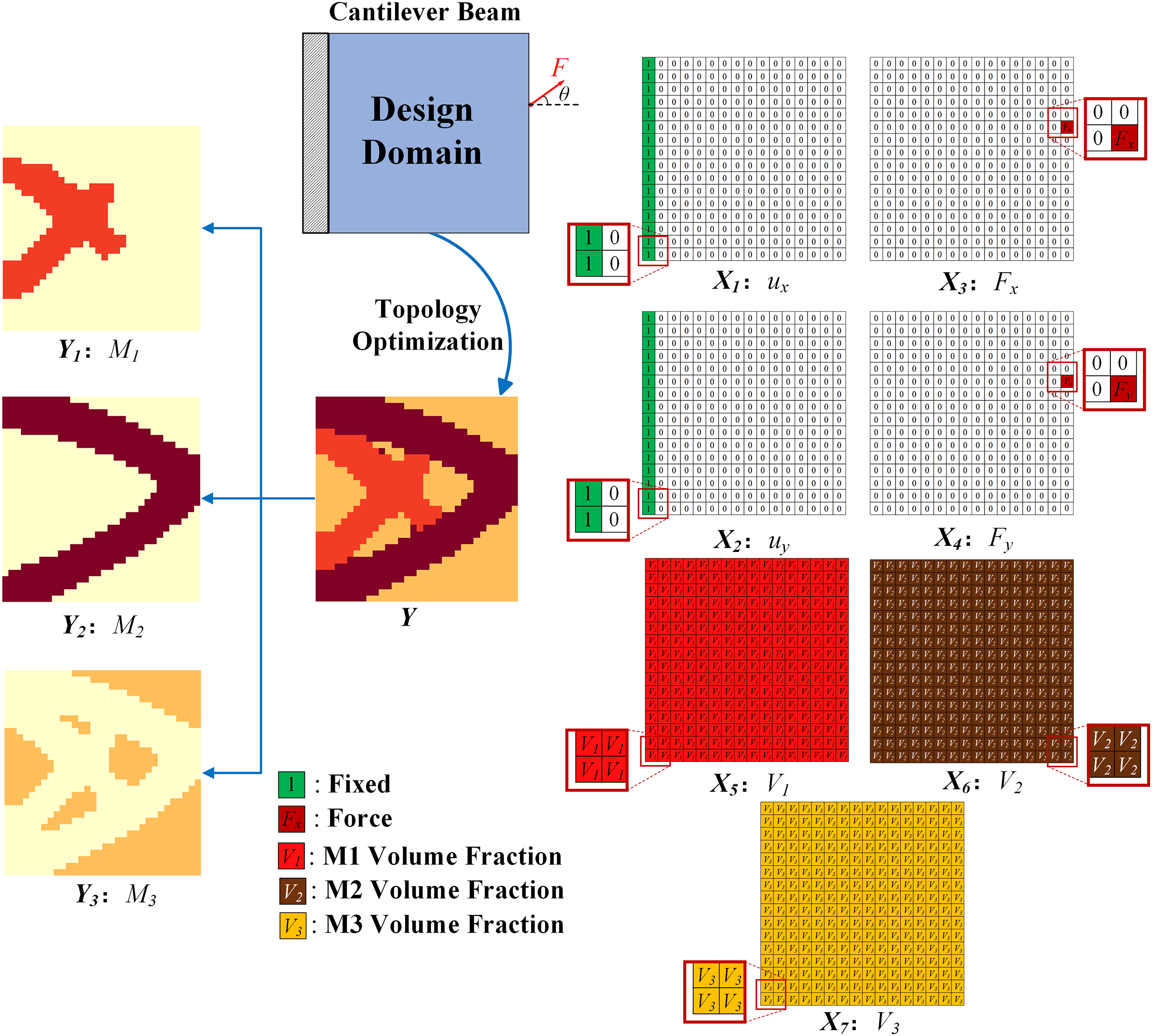
Figure 4: The input and output of neural network on the cantilever beam

Once the parameters are obtained, the 115 lines algorithm [69] is employed to generate samples with varying dataset scales, such as 3000, 6000, 12000, 18000, 24000, 30000, and so on. In this section, a novel approach is proposed to facilitate the learning of multimaterial constraints by generating data with multiple condition channels for the input and several channels with the same number of material types for the labels. As depicted in Fig. 4, each data can be represented as (X1, X2, X3, X4, X5, X6, X7, Y1, Y2, Y3), where (X1, X2, X3, X4, X5, X6, X7) and (Y1, Y2, Y3) serve as the input and labels for the neural network, respectively. The details of these channels are explained below. In the design domain, the number of elements and nodes is 32×32 and 33×33, respectively. The ten channels are: X1, X2, X3, and X4 with dimensions of 33×33, and X5, X6, X7, Y1, Y2, Y3 with dimensions of 32×32. The values of the fixed nodes and free nodes are represented as 1 and 0, respectively. The ux and uy matrices have a value of 0 everywhere except at the fixed nodes, where they have a value of 1 on the left-hand side. Similarly, the load matrices Fx and Fy have a value of 0 everywhere except at the node where the load force F is applied. At the loading node, the pixel values are Fx=Fcos⁡θ and Fy=Fsin⁡θ in the x and y directions, respectively. For the volume fraction channels (V1, V2, V3), each grid is filled with the corresponding material’s volume fraction. As the labels for the neural network, each matrix (M1, M2, M3) represents the distribution of the corresponding material.

For the other two classic topology optimization problems, the method and process of data generation are identical to those of the cantilever beam. However, it is worth noting that, apart from modifying the size of the design domains, the most significant variation lies in the load conditions. The loading parameters for the MBB beam are outlined below:

•   Loading position: the node chosen from the node set on the upper edge of the design domain

•   Loading direction: [180, 360°]

For the Michell beam, the range of loading positions extends the lower edge of the design domain in comparison to the MBB beam.

To ensure effective training of the surrogate model and accurate performance evaluation, each dataset is partitioned into three subsets: the training set (80%), the validation set (10%), and the test set (10%).

3.3 Network Architecture

The chosen network architecture for model training is the feature pyramid network [72], which is a well-known convolutional neural network [73–75] integrated with a feature pyramid framework. The FPN employs a top-down architecture with lateral connections to effectively capture multi-scale information, enhancing the accuracy of prediction results. According to the characteristics of neural network model, the size and number of input and output channels of the same surrogate model are basically fixed. In this section, we will describe the details of the network architecture using the dataset generated by the nx×ny=32×32 cantilever beam described in Section 3.2 as an object. As shown in Fig. 5, we use the 33×33×7 dimensional channel generated by the cantilever beam as input to obtain the network architecture. Before the sample is fed into the neural network, the three channels (X5, X6, X7) about volume fraction have been filled from 32×32 to 33×33 with rows and columns all zeros, just like the filling process in convolution operations. Here, keeping the dimensions of all input channels consistent is easy to calculate and ensures that convolution operations are not error-prone. In this study, the convolution operation details of the specific FPN architecture are shown in Fig. 5. It comprises four main components: bottom-up pathway, top-down pathway, lateral connections, and aggregation.

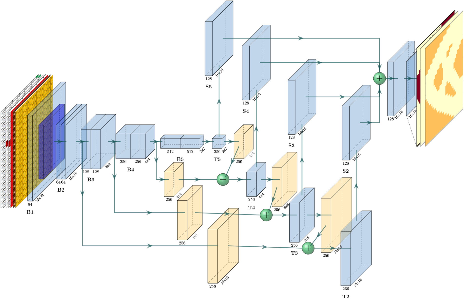
Figure 5: The architecture of FPN for the cantilever beam

Bottom-up pathway. The bottom-up pathway involves the extraction of features using a downsampling strategy, resulting in a substantial reduction in the size of the feature maps at each layer. These feature maps at different layers collectively form multi-scale feature maps that effectively capture the inherent law in the data. In this study, the ResNet18 [76] is employed as the backbone of the architecture. As depicted in Fig. 5, the bottom-up pathway consists of five major layers denoted as {B1, B2, B3, B4, B5}. Before the top-down pathway, the 33×33×7 dimensional input channel of the network is converted to B1 (32×32×7) by using a 2×2 convolutional layer. Subsequently, B1 is transformed into B2 through the utilization of a downsample block depicted in Fig. 6a. The bottom-up pathway then acquires B3, B4, and B5 by reusing the aforementioned downsample block.

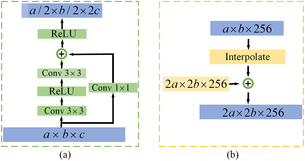
Figure 6: Two kinds of building block: (a) downsample block, (b) upsample block

Top-down pathway. The lower-level feature map can be derived from the higher-level feature map by employing an up-sampling technique. Furthermore, the fusion of high-level semantic information and low-level details is achieved through lateral connections in the feature maps. As depicted in Fig. 5, the top-down pathway primarily comprises four layers denoted as {T2, T3, T4, T5}. Specifically, B5 employs a convolution operation with a 1×1 convolutional layer to generate T5. Subsequently, T5 is further processed to yield T4 through the utilization of an upsample block illustrated in Fig. 6b. The upsample block is then reused to sequentially obtain T3 and T2.

Lateral connections. Fig. 5 illustrates that the yellow layers and green balls play a crucial role in the implementation of lateral connections. Within the lateral connection, a convolutional layer with a 1×1 kernel is utilized to reduce the dimension through element-wise addition between the upper and lower feature maps. Here, all lateral connections have a number of 256 channels.

Aggregation. Because the feature maps at various levels of the top-down pathway have different sizes, the sets {S2, S3, S4, S5} are generated through multiple convolutions using a convolution layer with 3×3 kernel, resulting in feature maps of size 16×16. As depicted in Fig. 5, S2, S3, S4, and S5 of equal size and dimension are aggregated using an addition operation. By employing a convolutional layer with a 1×1 kernel, the dimension of the aggregated feature maps is reduced to match the number of label channels for prediction. Consequently, the final output of the network model is 32×32×3, where each channel represents a material distribution. Through the combination of three channels, the final optimal structure is obtained.

3.4 Loss Function

For the rapid solution of multi-material topology optimization problems using neural networks, model training can be approached as either an image-to-image regression task or a classification task. The choice of the loss function plays a crucial role in distinguishing between these two types of tasks. As the loss functions, two commonly used error metrics for regression tasks, MSE and MAE are applied. MSE measures the squared error between the predicted value and the ground truth. MAE measures the absolute error between the estimated value and the ground truth. The formulations for two loss functions are as follows:

LMSE=1pN∑i=1p∑e=1N(y^ie−yie)2(11)

LMAE=1pN∑i=1p∑e=1N|y^ie−yie|(12)

where LMSE and LMAE represent the error values calculated for MSE and MAE, respectively. p represents the number of material categories, and N represents the number of grid elements. y^ie represent the predicted value, and yie is the target value. Noted that two models with the same architecture but different loss functions are used, which will produce varying predictions because different loss functions provide individual mapping strategies [77]. Despite both models being regression tasks, the prediction performance of the two loss functions is evaluated using diverse datasets for comparison purposes.

The cross-entropy loss function is commonly employed in classification tasks. The main goal of the cross entropy loss function is to maximize the probability of the correct predictions using the principle of maximum likelihood. Similarly, in this study, we adopt the CEL as the loss function for multi-material problems. The formulation of the cross-entropy loss function is presented below:

LCEL=−1PN∑i=1p∑e=1Nyielog⁡(y^ie)(13)

In the above equation, LCEL represents the calculated metric value for CEL. The parameters used in Eq. (13) are the same as those in Eqs. (11) and (12). Specifically, the binary cross-entropy (BCE) function is employed as the loss function for binary classification problems. Although BCE is typically used for binary classification, it has been successfully applied to topology optimization and obtains high precision results [45,51,78]. Notably, our work pioneers the application of CEL to solve multi-classification problems in the context of multi-material topology optimization.

3.5 Evaluating Metrics

To evaluate the performance of the surrogate model reasonably, we utilize three metrics: the relative error of compliance (REC), the relative error of volume fraction (REV), and the MAE-based prediction accuracy (ACC). Among these metrics, ACC is the most indicative metrics in this study. The definitions of these metrics are as follows:

1.   REC is defined as the relative error of the compliance between the predicted structure Y^ and the ground-truth structure Y.

REC=|C(Y^)−C(Y)|C(Y)(14)

2.   REV is the relative error of the volume fraction between the predicted structure Y^ and the ground-truth structure Y.

Total Volume=∑i=1pVi=1(15)

Vi=1N∑e=1Nyie(16)

REV =∑i=1p|V^i−Vi|Total Volume=∑i=1p|1N∑e=1N(y^ie−yie)|(17)

where Vi represents the prescribed volume fraction corresponding to phase i-th, and V^i represents the volume fraction of phase i-th in the prediction structure.

3.   During the process of model training, as well as after its completion, validation sets and test sets are employed to evaluate the performance of the model. The accuracy performance, which is evaluated based on MAE, is defined in Eq. (18). The defined accuracy expression is suitable for both regression tasks and classification tasks.

ACC=1−MAE=1−1pN∑i=1p∑e=1N|y^ie−yie|(18)

4  Experiment Results and Discussion

In this section, we begin by employing a widely used dataset of cantilever beams as the research objects to assess the performance of the surrogate model. Subsequently, we investigate the connection between topology optimization problems and the prediction accuracy, while also examining the impact of training data scale on the prediction performance. The model training is implemented using a single NVIDIA TITAN RTX card equipped with 32 GB of device memory, utilizing the Python open-source package (PyTorch 1.4). We choose Adam [79] as the optimizer method to train the models.

4.1 Performance of the Surrogate Model

In this section, we assess the performance of the FPN model by selecting a dataset consisting of 6000 generated from 32×32 dimensional cantilever beams as the research object. Subsequently, three loss functions, namely MSE, MAE, and CEL, are employed to train the FPN model, yielding distinct surrogate models. The setting of hyperparameters directly affects the performance of the neural network model, but it cannot be updated by itself during training. In order to obtain the best model generalization performance, model training needs to be terminated when overfitting begins. This experiment prevents overfitting by using an early stopping method. Specifically, the model training will be terminated if the validation accuracy (ACC) does not improve during 5 consecutive epochs. The maximum training condition of this study is set at 500 epochs. After several experiments to explore the hyperparameters, we set the batch size to 64 and the learning rate to 0.01 for each model.

Firstly, we examine the training performance of the FPN model, and the convergence history of the loss value throughout the process with different loss functions is depicted in Fig. 7. The curves displayed in Fig. 7 demonstrate that all three surrogate models exhibit stable convergence performance in both the training set and the validation set. Additionally, these models demonstrate minimal discrepancies between the validation loss and training loss. As the number of training epochs increases, the results generated by the three FPN models approach the ground-truth results in terms of quality. Regarding the comparison of convergence speed in this experiment, the MSE-Network exhibits the fastest convergence, while the CEL-Network demonstrates the slowest convergence. Three FPN models achieve relatively stable convergence within the initial 80 epochs, eventually converging to the following values: MSE training loss of 0.009, MSE validation loss of 0.017, MAE training loss of 0.028, MAE validation loss of 0.041, CEL training loss of 0.596, and CEL validation loss of 0.605. It is important to note that different types of surrogate models can not directly compare the value of the loss function to judge the performance due to the distinct principles of loss function composition. Therefore, a comprehensive analysis of the performance of the three surrogate models is provided in Fig. 8.

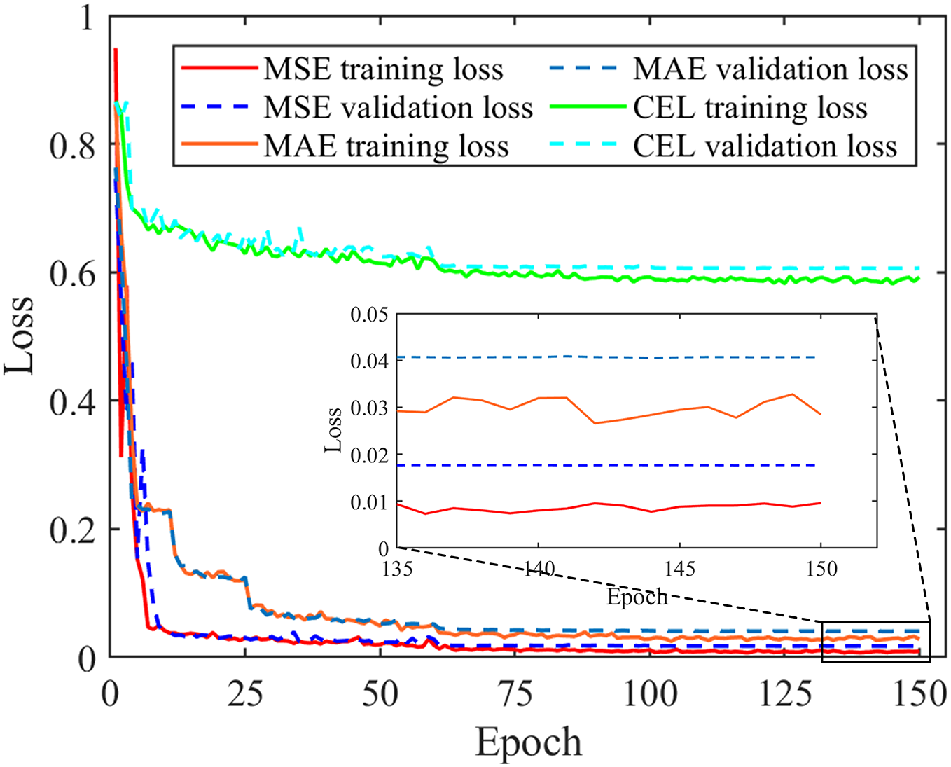
Figure 7: The convergence history of the loss value throughout the process with different loss function

Figure 8: Metrics comparison of using different loss function in the validation set

Fig. 8 illustrates the convergence history of the three metrics (REC, REV, ACC) for the FPN models, with each metric calculated as the mean value of all validation samples. As depicted in Figs. 8a and 8b, the REC values for the MSE-Network, MAE-Network, and CEL-Network gradually converge to 0.0096, 0.0186, and 0.0395, respectively. Similarly, the REV values for the three models gradually converge to 0.0200, 0.0250, and 0.0440, respectively. The order observed in both REC and REV metrics is consistent, with the MSE-Network exhibiting the smallest error and the CEL-Network displaying the largest error among the three models. Furthermore, Fig. 8c clearly demonstrates that the ACC values obtained by the MSE-Network, MAE-Network, and CEL-Network ultimately converge stably to 0.9530, 0.9590, and 0.9580, respectively. It is worth noting that the order of ACC values differs from that of REV and REC, indicating a relatively independent nature of the three metrics within each model. Initially, the convergence history of the metrics for all three models exhibited significant fluctuations. However, as the model training progressed, all the aforementioned metrics tended to converge steadily.

Based on the statistics presented in Fig. 8, all three models have presented a good performance on computing the new samples in the validation set. This not only demonstrates the feasibility of the FPN architecture for surrogate modeling but also highlights the effectiveness of the developed models in predicting the optimized multiphase structures under diverse condition parameters.

Fig. 9 displays the structures generated by the traditional method and the FPN models, along with their corresponding metrics listed below. As observed in Fig. 9, the structures produced by the different FPN models closely align with the ground-truth structures. Additionally, Most of the structures obtained by FPN model show remarkable similarity with the ground-truth. as indicated by high accuracy values (REC and REV both less than 0.05, and ACC greater than 95%). This suggests that the developed surrogate models possess a high level of prediction precision. Upon comparing the evaluation metrics of the results from the three FPN models, it is evident that the prediction precision of the MSE-Network and MAE-Network slightly surpasses that of the CEL-Network. Furthermore, the prediction precision of the MSE-Network and MAE-Network is nearly identical. This implies that regression tasks perform marginally better than classification tasks in the surrogate modeling of multi-material topology optimization problems. However, the applicability of this observation to a broader range of multi-material topology optimization problems requires further verification and investigation through additional experiments.

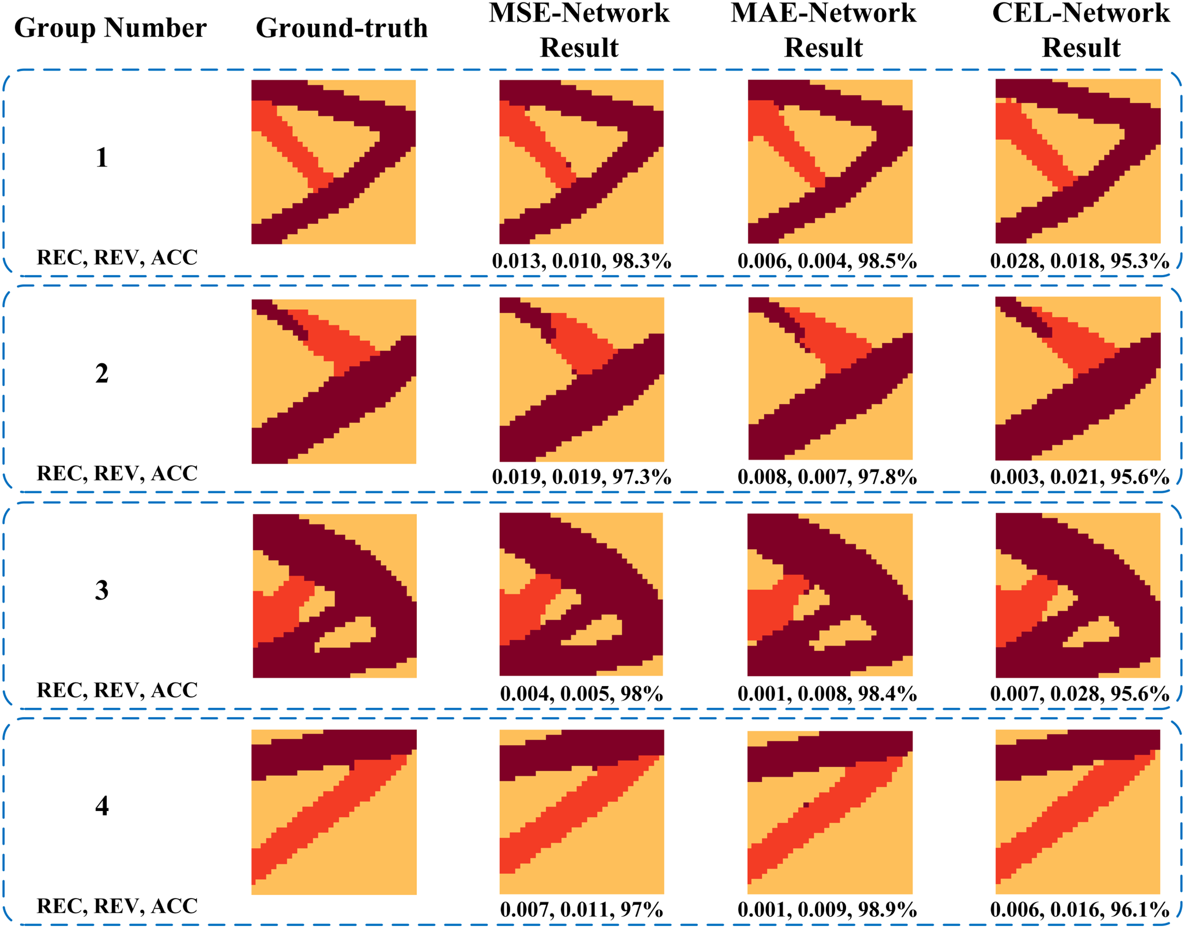
Figure 9: Comparison of results between the ground-truth and prediction of FPN models

4.2 The Relationship between Topology Optimization Problems and the Prediction Performance

This section introduces twelve cases to examine the correlation between various topology optimization problems and the prediction performance of FPN surrogate models. The specific parameters for all cases are provided in Table 1. It can be observed from Table 1 that three classical TO problems (cantilever beam, MBB beam, and Michell beam) are chosen as research subjects. These problems encompass different design domain sizes, loading positions, fixed positions, and material category quantities, resulting in the generation of a dataset comprising 6000 samples for each problem. It is noteworthy that we employ MATLAB with 16 cores for parallel computation to generate the datasets. The dataset generation process exhibits a relatively swift performance. For instance, the generation of 6000 data samples for Case4 in Table 1, which represents the cantilever beam with the highest resolution and the maximum number of material category, is accomplished within a mere 4.47 min. Similarly, the data set generation of Case8 (MBB beam) and Case12 (michell beam) requires the longest duration in the same class of topology optimization problems. Specifically, dataset generation of Case8 consumes 9.21 min, while dataset generation of Case12 takes 8.34 min. Despite the time required for dataset generation, the overall time consumption remains within an acceptable range. The hyperparameter settings for the model training process in this section are the same as in Section 4.1

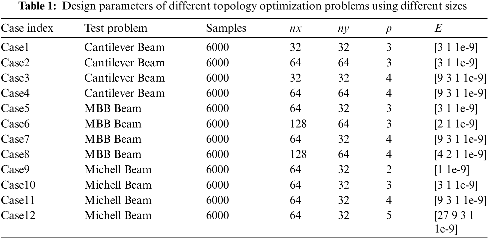
Fig. 10 presents the performance of different FPN surrogate models using various cases from the test set. By comparing the experimental results of Case1 to Case4, it is observed that the prediction precision of Case1 and Case2 is nearly identical, as is the case for Case3 and Case4. However, the prediction precision of Case1 to Case2 is superior to that of Case3 to Case4. This suggests that changes in design domain sizes do not significantly impact the prediction precision of the surrogate models, while an increase in material category quantities leads to a decrease in prediction precision for the same topology optimization problem. Similarly, even though the research domain transitions from a cantilever beam to an MBB beam, the experimental results of Case5 to Case8 still exhibit the same pattern. Here, we assume that the Young’s modulus (E) does not affect the prediction precision, as it does not participate in the model training. This assumption is validated by the experimental results of Case5 to Case8, where the change in Young’s modulus (E) from [3, 1, 1e-9] to [2, 1, 1e-9] does not impact the pattern observed in Case1 to Case4. Therefore, to further assess the influence of material category quantities on prediction precision, Case9 to Case12 are designed to utilize four different material category quantities for the Michell beam. Clearly visible in Case9 to Case12 of Fig. 10 is the continuous decrease in prediction precision as the material category quantities increase from 2 to 5. This can be attributed to the increase in the number of input and output channels of the model as the material category quantities increase, thereby augmenting the mapping complexity and reducing the prediction precision.

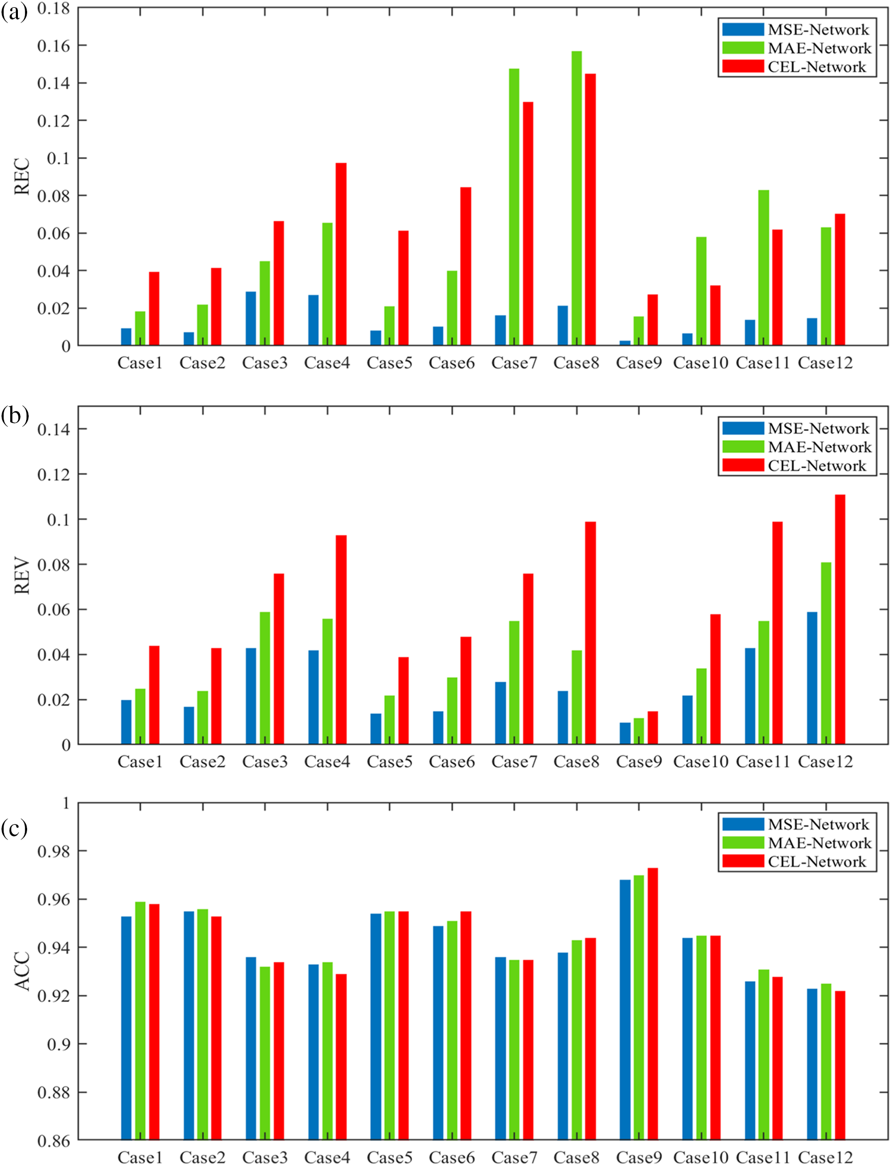
Figure 10: Performance of different FPN surrogate models using different topology optimization problems in the test set. Case1 to Case4, Case5 to Case8, and Case9 to Case12 consist of cantilever beams, MBB beams, and Michell Beams, respectively. (a) REC, (b) REV, (c) ACC

In Fig. 10, when comparing the three FPN models within each case, it is evident that the ACC values of the three models are nearly identical. However, the REV values of MSE-Network, MAE-Network, and CEL-Network gradually increase. Meanwhile, the size comparison of REC values of the three models is similar to the law of REV values in most cases. If the prediction precision of the surrogate models is solely based on the ACC value, the three FPN models are essentially equivalent. However, when considering the REC and REV values, it becomes apparent that MSE-Network exhibits the highest prediction precision, while CEL-Network demonstrates the lowest prediction precision among the three FPN models. This finding indicates that the regression task outperforms the classification task in surrogate modeling for multi-material topology optimization problems, further supporting the conclusion drawn in Section 4.1.

Fig. 11 showcases several examples of ground-truth and predicted structures, along with the problem definition parameters, volume fractions, and prediction metrics. It is evident from Fig. 11 that all three FPN models achieve a high prediction precision of over 95% in each example. Additionally, the metrics (REC, REV, and ACC) of MSE-Network and MAE-Network generally outperform those of CEL-Network in most examples. For instance, in Example 2, the REC values for MSE-Network, MAE-Network, and CEL-Network are 0.006, 0.002, and 0.013, respectively. Similarly, the REV values for these models are 0.017, 0.029, and 0.056, respectively. Furthermore, the ACC values for these models are 98.1%, 97.5%, and 95.3%, respectively, which is the most representative metric among the three. This observation highlights that, when evaluating surrogate modeling based on the evaluation metrics, the regression task exhibits a slight superiority over the classification task.

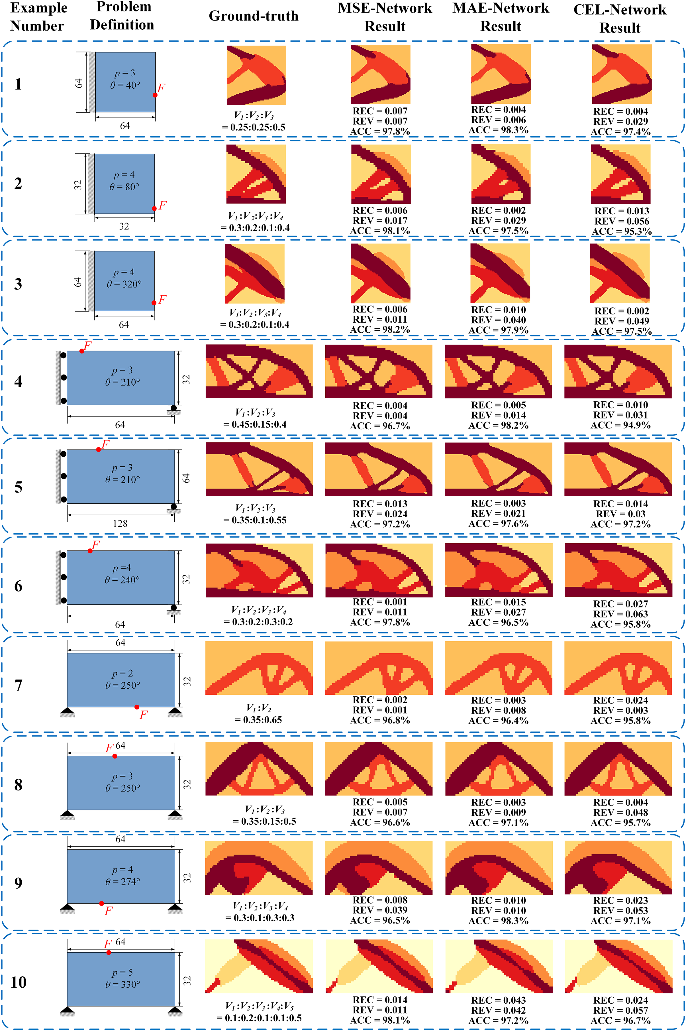
Figure 11: Comparisons between the ground-truth and the prediction of different FPN models

The trained surrogate model enables rapid predictions of structural topology. In this part, we present a comparative analysis between the surrogate model and traditional methods [69] to highlight the speed advantage. It is important to emphasize that once the model is trained, the choice of loss function has no impact on the prediction speed. Consequently, there are no significant differences in the prediction speed among the MSE-Network, MAE-Network, and CEL-Network trained from the same dataset. As a result, we typically select a representative surrogate model from the three options to assess prediction time. For instance, in Example 1 of Fig. 11, the traditional method required 8.98 s to solve the topology, whereas the MSE-Network prediction took only 0.011 s. The traditional method took 816 times longer than the surrogate model. Similarly, in Example 4, the traditional algorithm took 16.21 s, whereas the MSE-Network prediction only consumed 0.010 s. In this case, the traditional method took 1621 times longer than the surrogate model. These findings demonstrate that the surrogate model achieves significantly shorter prediction times compared to traditional methods, as it eliminates the need for finite element solving and multiple iterations. Through multiple experiments, we consistently observed that the prediction time of the surrogate model remains around 0.01 s, regardless of variations in the design domain resolution and the number of material category. This indicates that the prediction time of the surrogate model is independent of the specific topology optimization problem.

4.3 The Relationship between the Training Data Scale and the Prediction Accuracy

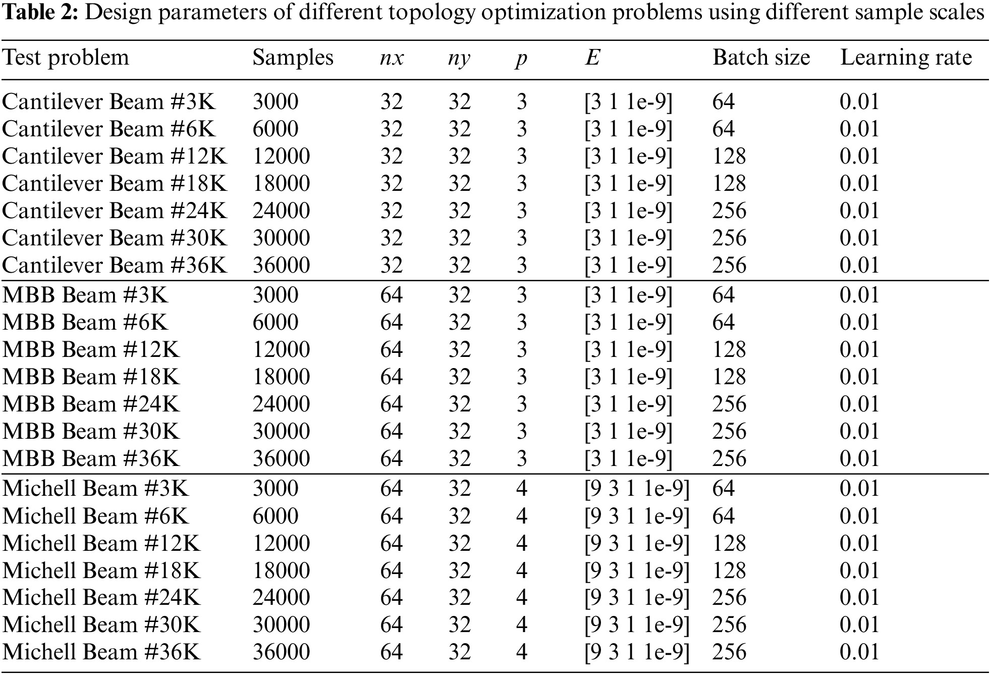
In this section, we investigate the impact of the training dataset scale on the prediction performance. To accomplish this, we select three topology optimization problems and generate datasets with varying data scales for training the models. The dataset scales considered are 3000, 6000, 12000, 18000, 24000, 30000, and 36000. Table 2 presents the design parameters corresponding to each dataset scale, including design domain sizes, the quantities of material categories, and the hyperparameters of the model training. Each cantilever beam or MBB beam sample comprises seven input channels and a label with three channels. On the other hand, each Michell beam sample consists of eight input channels and a label with four channels. To assess the learning capability of the proposed model across different topology optimization problems, the experiments involving the cantilever beam and MBB beam utilize samples with the same quantities of material categories. Furthermore, the Michell beam, which incorporates four different materials, is chosen as an experimental subject to examine the learning law and adaptability of the FPN models with respect to changes in the quantities of material categories.

The experimental results are summarized in Fig. 12. As depicted in the figure, a clear trend in the prediction precision can be observed. Overall, the prediction precision of the developed models improves as the data scale increases. These results demonstrate that larger sample scales lead to higher prediction precision of the FPN models. The performance of the models confirms that training the surrogate model with a larger number of samples results in better prediction precision, assuming that other parameters remain constant. Furthermore, Fig. 12 reveals three main laws or characteristics.

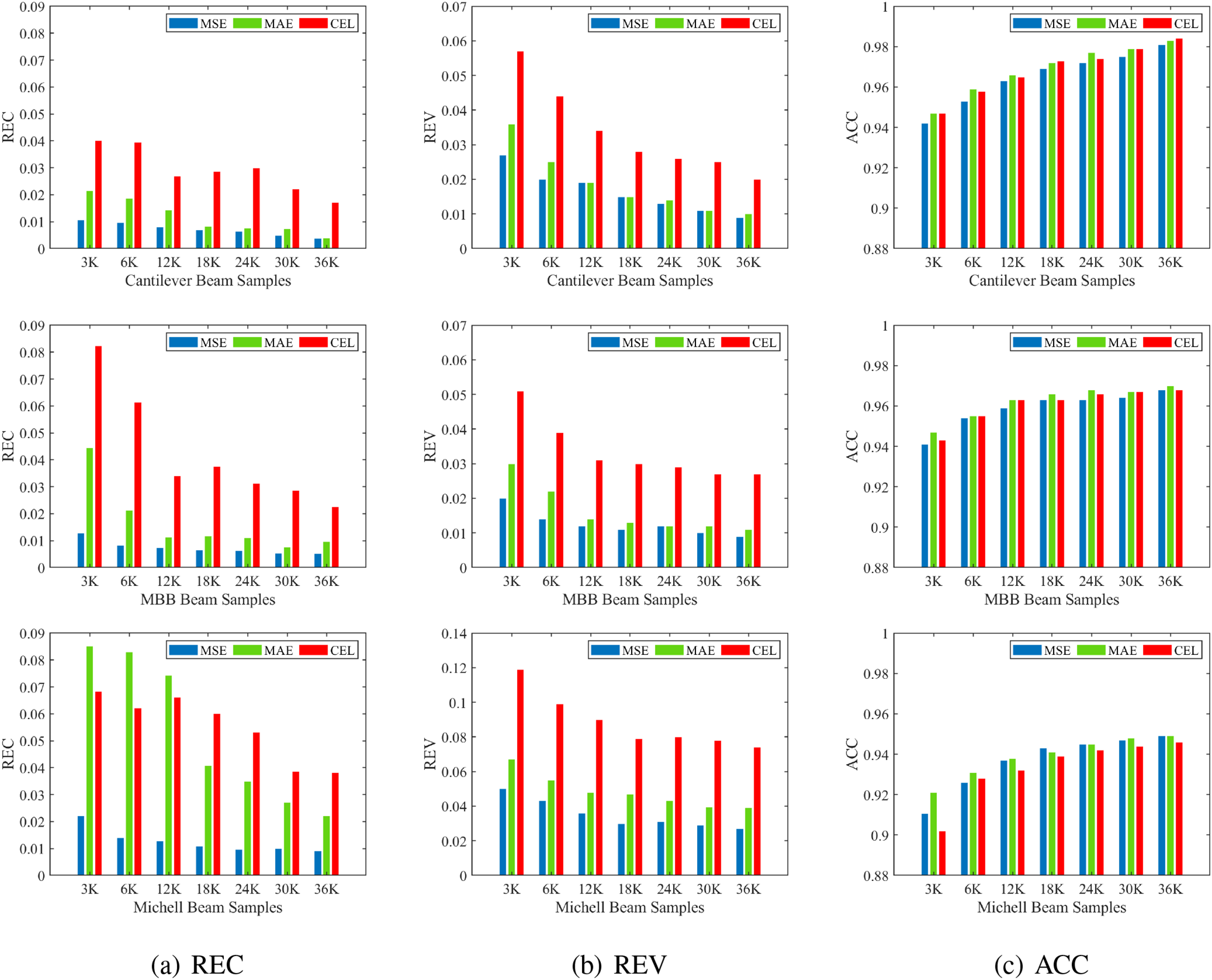
Figure 12: Performance of different FPN surrogate models using different sample scales in the test set

First and foremost, it is evident that the prediction precision of the obtained surrogate models varies for different topology optimization problems, even when the sample scale remains the same. For instance, in the case of the CEL-Network, the REC values for Cantilever Beam #3K and MBB Beam #3K are 0.0401 and 0.0823, respectively. This discrepancy can be attributed to the fact that the datasets generated by different topology optimization problems contain distinct information. Consequently, the parameters in the obtained surrogate models differ, leading to variations in the prediction precision. Moreover, when the data scale increases by the same magnitude, the improvement in prediction precision varies across different surrogate models. For example, when comparing the test cases ranging from Cantilever Beam #3K to Cantilever Beam #36K, the REC values of the CEL-Network decreased by 57.6%. However, when examining the test cases ranging from MBB Beam #3K to MBB Beam #36K, the REC values of the CEL-Network decreased by 72.5%.

Secondly, it is evident from Fig. 12 that the MSE-Network consistently achieves the highest prediction precision in most cases, while the CEL-Network exhibits the lowest prediction precision among the three surrogate models obtained from the same dataset. As the data scale of a given TO problem increases, the effect of improving prediction precision varies across the three surrogate models. In general, the prediction precision of the MSE-Network shows a slight improvement, maintaining its position as the model with the highest prediction accuracy among the three models. On the other hand, the improvement in prediction precision of the MAE-Network demonstrates its unique characteristics. Initially, when the data scale is small (Cantilever Beam #3K), the prediction precision of the MAE-Network is significantly lower than that of the MSE-Network. However, as the data scale gradually increases, the precision gap between the MAE-Network and MSE-Network diminishes step by step, eventually resulting in almost identical prediction precision in the two models (Cantilever Beam #36K). Furthermore, with the increase in sample scale, it is evident from the red bar chart in Fig. 12a that the precision improvement of the CEL-Network is accompanied by some degree of volatility. This phenomenon may be attributed to the fact that the output of the classification task lacks intermediate transitional values that are present in the output of the regression task.

Last but not least, in the FPN models trained using Michell beam samples, the minimum and maximum ACC values were 90.2% and 94.9%, respectively. However, in the models obtained from cantilever beam or MBB beam samples, the minimum ACC value exceeds 94%, and the maximum ACC value can reach 98.4%. Similarly, the REC and REV metrics also follow the same trend. This discrepancy can be attributed to the fact that cantilever beam or MBB beam samples are generated from three materials, whereas Michell beam samples are generated from four materials. Therefore, it can be concluded that the prediction precision of the FPN surrogate model decreases with an increase in the number of sample materials, as also discussed in Section 4.2.

5  Conclusions

This paper focuses on the study of MMTO problems within the framework of multiphase topology optimization using deep learning. For the first time, a CNN model is employed to construct a surrogate model capable of predicting multi-material structural topologies with respect to different conditional parameters. The key innovation of this research lies in the introduction of a coding method that efficiently integrates the multi-material topology optimization problem with neural networks. The obtained surrogate model enables rapid generation of multi-material structural topologies without the need for iterative processes or the finite element analysis. Then, the solution time of the surrogate model remains unaffected by the size of the design domain or the number of material categories. To facilitate the learning process, a feature pyramid network is utilized to establish the mapping between the input parameter channel and the corresponding output structural topology. Experimental results demonstrate that the FPN surrogate models not only have high prediction precision but also have good generalization ability.

Furthermore, a framework is proposed to determine the most suitable surrogate model mapping for both regression and classification tasks. This framework aims to identify the surrogate model that achieves high accuracy within the same dataset. Extensive experimental results demonstrate that both regression and classification tasks can be employed as surrogate model mappings. However, in most cases, the mapping constructed as a regression task outperforms the classification task. Regarding the regression task, when dealing with small-scale data, the prediction accuracy of the MSE-Network slightly surpasses that of the MAE-Network. As the data scale increases, the prediction accuracy of the MSE-Network becomes nearly identical to that of the MAE-Network. Overall, the MSE-Network exhibits the best prediction performance among the MSE-Network, MAE-Network, and CEL-Network.

In addition to selecting the FPN models and configuring the hyperparameters, the experimental results highlight several factors that influence the prediction accuracy of the surrogate model. These factors primarily include the topology optimization problems, material category quantities, and the data scales, while the irrelevant factors mainly include the domain size and the elastic modulus of the material. Based on the findings, two general trends can be summarized. Firstly, an increase in the quantity of material categories tends to decrease the prediction accuracy of surrogate models. Secondly, a larger volume of training data leads to improved performance of the surrogate models.

In future work, we aim to expand the application of 2D multi-material topology optimization to 3D multi-material topology optimization problems. Furthermore, we are conducting further research on the utilization of surrogate models and multi-materials method in multi-scale structural design. The surrogate model based on neural networks offers a practical approach to expedite the analysis of macro and micro structure properties. Simultaneously, the integration of multi-material design caters to the diverse and functional requirements of microstructures, thereby accommodating a broader range of design possibilities.

Acknowledgement: The authors gratefully acknowledge the support provided by the National Natural Science Foundation of China and Postgraduate Scientific Research Innovation Project of Hunan Province. The author also expresses gratitude to all the anonymous reviewers.

Funding Statement: This work was supported in part by National Natural Science Foundation of China under Grant Nos. 51675525, 52005505, and 62001502, and Post-Graduate Scientific Research Innovation Project of Hunan Province under Grant No. XJCX2023185.

Author Contributions: The authors confirm contribution to the paper as follows: study conception and design: Jiaxiang Luo, Bingxiao Du, Wen Yao; data collection: Jiaxiang Luo, Weien Zhou; analysis and interpretation of results: Jiaxiang Luo, Daokui Li, Wen Yao; draft manuscript preparation: Jiaxiang Luo, Weien Zhou, Bingxiao Du. All authors reviewed the results and approved the final version of the manuscript.

Availability of Data and Materials: Data are available on request.

Conflicts of Interest: The authors declare that they have no conflicts of interest to report regarding the present study.

References

1. Bendsøe, M. P., Kikuchi, N. (1988). Generating optimal topologies in structural design using a homogenization method. Computer Methods in Applied Mechanics and Engineering, 71(2), 197–224. https://doi.org/10.1016/0045-7825(88)90086-2 [Google Scholar] [CrossRef]

2. Hassani, B., Hinton, E. (1998). A review of homogenization and topology optimization i-homogenization theory for media with periodic structure. Computers and Structures, 69(6), 707–717. https://doi.org/10.1016/S0045-7949(98)00131-X [Google Scholar] [CrossRef]

3. Bendsoe, M. P. (1989). Optimal shape design as a material distribution problem. Structural Optimization, 1(4), 193–202. https://doi.org/10.1007/BF01650949 [Google Scholar] [CrossRef]

4. Zhou, M., Rozvany, G. (1991). The coc algorithm, part ii: Topological, geometrical and generalized shape optimization. Computer Methods in Applied Mechanics and Engineering, 89(1), 309–336. [Google Scholar]

5. Rozvany, G. I. N., Zhou, M., Birker, T. (1992). Generalized shape optimization without homogenization. Structural Optimization, 4(3), 250–252. [Google Scholar]

6. Wang, M. Y., Wang, X., Guo, D. (2003). A level set method for structural topology optimization. Computer Methods in Applied Mechanics and Engineering, 192(1–2), 227–246. [Google Scholar]

7. Allaire, G., Jouve, F., Toader, A. M. (2004). Structural optimization using sensitivity analysis and a level-set method. Journal of Computational Physics, 194(1), 363–393. https://doi.org/10.1016/j.jcp.2003.09.032 [Google Scholar] [CrossRef]

8. Xie, Y. M., Steven, G. P. (1993). A simple evolutionary procedure for structural optimization. Computers Structures, 49(5), 885–896. https://doi.org/10.1016/0045-7949(93)90035-C [Google Scholar] [CrossRef]

9. Guo, X., Zhang, W., Zhong, W. (2014). Doing topology optimization explicitly and geometrically—a new moving morphable components based framework. Journal of Applied Mechanics, 81(8), 081009. https://doi.org/10.1115/1.4027609 [Google Scholar] [CrossRef]

10. Liu, C., Zhu, Y., Sun, Z., Li, D., Du, Z. et al. (2018). An efficient moving morphable component (MMC)-based approach for multi-resolution topology optimization. Structural and Multidisciplinary Optimization, 58, 2455–2479. https://doi.org/10.1007/s00158-018-2114-0 [Google Scholar] [CrossRef]

11. Bourdin, B., Chambolle, A. (2003). Design-dependent loads in topology optimization. ESAIM Control Optimisation and Calculus of Variations, 9, 19–48. https://doi.org/10.1051/cocv:2002070 [Google Scholar] [CrossRef]

12. Banga, S., Gehani, H., Bhilare, S., Patel, S., Kara, L. (2018). 3D topology optimization using convolutional neural networks. arXiv:1808.07440. [Google Scholar]

13. Xiang, C., Wang, D. L., Pan, Y., Chen, A. R., Zhou, X. L. et al. (2022). Accelerated topology optimization design of 3D structures based on deep learning. Structural and Multidisciplinary Optimization, 65(3), 99. https://doi.org/10.1007/s00158-022-03194-0 [Google Scholar] [CrossRef]

14. Chandrasekhar, A., Suresh, K. (2021). Multi-material topology optimization using neural networks. Computer-Aided Design, 136, 103017. https://doi.org/10.1016/j.cad.2021.103017 [Google Scholar] [CrossRef]

15. Du, Z., Guo, Y., Liu, C., Zhang, W., Xue, R. et al. (2024). Structural topology optimization of three-dimensional multi-material composite structures with finite deformation. Composite Structures, 328, 117692. https://doi.org/10.1016/j.compstruct.2023.117692 [Google Scholar] [CrossRef]

16. Liu, H., Qi, Y., Chen, L., Li, Y., Xiao, W. (2024). An efficient data-driven optimization framework for designing graded cellular structures. Applied Mathematical Modelling, 125, 574–598. https://doi.org/10.1016/j.apm.2023.10.020 [Google Scholar] [CrossRef]

17. Li, J., Pokkalla, D. K., Wang, Z. P., Wang, Y. (2023). Deep learning-enhanced design for functionally graded auxetic lattices. Engineering Structures, 292, 116477. https://doi.org/10.1016/j.engstruct.2023.116477 [Google Scholar] [CrossRef]

18. Wei, G., Chen, Y., Li, Q., Fu, K. (2023). Multiscale topology optimisation for porous composite structures with stress-constraint and clustered microstructures. Computer Methods in Applied Mechanics and Engineering, 416, 116329. https://doi.org/10.1016/j.cma.2023.116329 [Google Scholar] [CrossRef]

19. Chen, Z., Long, K., Zhang, C., Yang, X., Lu, F. et al. (2023). A fatigue-resistance topology optimization formulation for continua subject to general loads using rainflow counting. Structural and Multidisciplinary Optimization, 66(9), 210. https://doi.org/10.1007/s00158-023-03658-x [Google Scholar] [CrossRef]

20. Sigmund, O., Torquato, S. (1997). Design of materials with extreme thermal expansion using a three-phase topology optimization method. Journal of the Mechanics and Physics of Solids, 45(6), 1037–1067. https://doi.org/10.1016/S0022-5096(96)00114-7 [Google Scholar] [CrossRef]

21. Gibiansky, L. V., Sigmund, O. (2000). Multiphase composites with extremal bulk modulus. Journal of the Mechanics and Physics of Solids, 48(3), 461–498. https://doi.org/10.1016/S0022-5096(99)00043-5 [Google Scholar] [CrossRef]

22. Castro, G. A. (2002). Optimization of nuclear fuel reloading by the homogenization method. Structural and Multidisciplinary Optimization, 24(1), 11–22. https://doi.org/10.1007/s00158-002-0210-6 [Google Scholar] [CrossRef]

23. Bendsøe, M. P., Sigmund, O. (1999). Material interpolation schemes in topology optimization. Archive of Applied Mechanics, 69(9–10), 635–654. [Google Scholar]

24. Yin, L., Ananthasuresh, G. K. (2001). Topology optimization of compliant mechanisms with multiple materials using a peak function material interpolation scheme. Structural and Multidisciplinary Optimization, 23(1), 49–62. https://doi.org/10.1007/s00158-001-0165-z [Google Scholar] [CrossRef]

25. Zhou, S., Wang, M. Y. (2007). Multimaterial structural topology optimization with a generalized cahn-hilliard model of multiphase transition. Structural and Multidisciplinary Optimization, 33(2), 89–111. [Google Scholar]

26. Wang, M. Y., Wang, X. (2004). “Color” level sets: A multi-phase method for structural topology optimization with multiple materials. Computer Methods in Applied Mechanics and Engineering, 193(6/8), 469–496. [Google Scholar]

27. Wang, M. Y., Wang, X. (2005). A level-set based variational method for design and optimization of heterogeneous objects. Computer-Aided Design, 37(3), 321–337. https://doi.org/10.1016/j.cad.2004.03.007 [Google Scholar] [CrossRef]

28. Faure, A., Michailidis, G., Parry, G., Vermaak, N., Estevez, R. (2017). Design of thermoelastic multi-material structures with graded interfaces using topology optimization. Structural and Multidisciplinary Optimization, 56(4), 823–837. https://doi.org/10.1007/s00158-017-1688-2 [Google Scholar] [CrossRef]

29. Wang, Y., Luo, Z., Kang, Z., Zhang, N. (2015). A multi-material level set-based topology and shape optimization method. Computer Methods in Applied Mechanics and Engineering, 283, 1570–1586. https://doi.org/10.1016/j.cma.2014.11.002 [Google Scholar] [CrossRef]

30. Ghasemi, H., Park, H. S., Rabczuk, T. (2018). A multi-material level set-based topology optimization of flexoelectric composites. Computer Methods in Applied Mechanics & Engineering, 332, 47–62. https://doi.org/10.1016/j.cma.2017.12.005 [Google Scholar] [CrossRef]

31. Huang, X., Xie, Y. M. (2009). Bi-directional evolutionary topology optimization of continuum structures with one or multiple materials. Computational Mechanics, 43(3), 393–401. https://doi.org/10.1007/s00466-008-0312-0 [Google Scholar] [CrossRef]

32. Radman, A., Huang, X., Xie, Y. M. (2014). Topological design of microstructures of multi-phase materials for maximum stiffness or thermal conductivity. Computational Materials Science, 91, 266–273. https://doi.org/10.1016/j.commatsci.2014.04.064 [Google Scholar] [CrossRef]

33. Choi, J. S., Izui, K., Nishiwaki, S. (2012). Multi-material optimization of magnetic devices using an allen-cahn equation. IEEE Transactions on Magnetics, 48(11), 3579–3582. https://doi.org/10.1109/TMAG.2012.2201212 [Google Scholar] [CrossRef]

34. Rouhollah, T. (2014). Multimaterial topology optimization by volume constrained allen-cahn system and regularized projected steepest descent method. Computer Methods in Applied Mechanics and Engineering, 276, 534–565. https://doi.org/10.1016/j.cma.2014.04.005 [Google Scholar] [CrossRef]

35. Montemurro, M., Rodriguez, T., Pailhès, J., Le Texier, P. (2023). On multi-material topology optimisation problems under inhomogeneous neumann-dirichlet boundary conditions. Finite Elements in Analysis and Design, 214, 103867. https://doi.org/10.1016/j.finel.2022.103867 [Google Scholar] [CrossRef]

36. Zhang, Y., Peng, B., Zhou, X., Xiang, C., Wang, D. (2019). A deep convolutional neural network for topology optimization with strong generalization ability. arXiv:1901.07761. [Google Scholar]

37. Abueidda, D. W., Koric, S., Sobh, N. A. (2020). Topology optimization of 2D structures with nonlinearities using deep learning. Computers & Structures, 237, 106283. https://doi.org/10.1016/j.compstruc.2020.106283 [Google Scholar] [CrossRef]

38. Zhang, Z., Liu, Q., Wang, Y. (2017). Road extraction by deep residual U-Net. IEEE Geoscience and Remote Sensing Letters, 99, 1–5. [Google Scholar]

39. Li, B., Huang, C., Li, X., Zheng, S., Hong, J. (2019). Non-iterative structural topology optimization using deep learning. Computer-Aided Design, 115, 172–180. https://doi.org/10.1016/j.cad.2019.05.038 [Google Scholar] [CrossRef]

40. Yan, J., Zhang, Q., Xu, Q., Fan, Z., Li, H. et al. (2022). Deep learning driven real time topology optimisation based on initial stress learning. Advanced Engineering Informatics, 51, 101472. https://doi.org/10.1016/j.aei.2021.101472 [Google Scholar] [CrossRef]

41. Wang, D., Cheng Xiang, Y. P. A. C. X. Z., Zhang, Y. (2022). A deep convolutional neural network for topology optimization with perceptible generalization ability. Engineering Optimization, 54(6), 973–988. https://doi.org/10.1080/0305215X.2021.1902998 [Google Scholar] [CrossRef]

42. Lei, X., Liu, C., Du, Z., Zhang, W., Guo, X. (2018). Machine learning driven real time topology optimization under moving morphable component (MMC)-based framework. Journal of Applied Mechanics, 86(1), 011004. [Google Scholar]

43. Yu, Y., Hur, T., Jung, J., Jang, I. G. (2019). Deep learning for determining a near-optimal topological design without any iteration. Structural and Multidisciplinary Optimization, 59(3), 787–799. https://doi.org/10.1007/s00158-018-2101-5 [Google Scholar] [CrossRef]

44. Nakamura, K., Suzuki, Y. (2020). Deep learning-based topological optimization for representing a user-specified design area. arXiv:2004.05461. [Google Scholar]

45. Ates, G. C., Gorguluarslan, R. M. (2021). Two-stage convolutional encoder-decoder network to improve the performance and reliability of deep learning models for topology optimization. Structural and Multidisciplinary Optimization, 63(4), 1927–1950. https://doi.org/10.1007/s00158-020-02788-w [Google Scholar] [CrossRef]

46. Sasaki, H., Igarashi, H. (2019). Topology optimization accelerated by deep learning. IEEE Transactions on Magnetics, 55(6), 1–5. [Google Scholar]

47. Lee, S., Kim, H., Lieu, Q. X., Lee, J. (2020). CNN-based image recognition for topology optimization. Knowledge-Based Systems, 198, 105887. https://doi.org/10.1016/j.knosys.2020.105887 [Google Scholar] [CrossRef]

48. Chi, H., Zhang, Y., Tang, T. L. E., Mirabella, L., Dalloro, L. et al. (2021). Universal machine learning for topology optimization. Computer Methods in Applied Mechanics and Engineering, 375, 112739. https://doi.org/10.1016/j.cma.2019.112739 [Google Scholar] [CrossRef]

49. Keshavarzzadeh, V., Kirby, R. M., Narayan, A. (2021). Robust topology optimization with low rank approximation using artificial neural networks. Computational Mechanics, 68(6), 1297–1323. https://doi.org/10.1007/s00466-021-02069-3 [Google Scholar] [CrossRef]

50. Qian, C., Ye, W. (2021). Accelerating gradient-based topology optimization design with dual-model artificial neural networks. Structural and Multidisciplinary Optimization, 63(4), 1687–1707. https://doi.org/10.1007/s00158-020-02770-6 [Google Scholar] [CrossRef]

51. Sosnovik, I., Oseledets, I. (2017). Neural networks for topology optimization. Russian Journal of Numerical Analysis and Mathematical Modelling, 34(4), 1–13. [Google Scholar]

52. Joo, Y., Yu, Y., Jang, I. G. (2021). Unit module-based convergence acceleration for topology optimization using the spatiotemporal deep neural network. IEEE Access, 9, 149766–149779. https://doi.org/10.1109/ACCESS.2021.3125014 [Google Scholar] [CrossRef]

53. Samaniego, E., Anitescu, C., Goswami, S., Nguyen-Thanh, V. M., Guo, H. et al. (2019). An energy approach to the solution of partial differential equations in computational mechanics via machine learning: Concepts, implementation and applications. Computer Methods in Applied Mechanics & Engineering, 362, 112790. [Google Scholar]

54. Wang, C., Yao, S., Wang, Z., Hu, J. (2020). Deep super-resolution neural network for structural topology optimization. Engineering Optimization, 53, 2108–2121. [Google Scholar]

55. Goodfellow, I., Pouget-Abadie, J., Mirza, M., Xu, B., Warde-Farley, D. et al. (2014). Generative adversarial nets. Proceeding of the Advances in Neural Information Processing Systems, 27, 2672–2680. [Google Scholar]

56. Rawat, S., Shen, M. H. H. (2019). A novel topology design approach using an integrated deep learning network architecture. arXiv:1808.02334. [Google Scholar]

57. Rawat, S., Shen, M. H. H. (2019). A novel topology optimization approach using conditional deep learning. arXiv:1901.04859. [Google Scholar]

58. Rawat, S., Shen, M. H. (2019). Application of adversarial networks for 3D structural topology optimization. WCX SAE World Congress Experience, SAE International. [Google Scholar]

59. Oh, S., Jung, Y., Kim, S., Lee, I., Kang, N. (2019). Deep generative design: Integration of topology optimization and generative models. Journal of Mechanical Design, 141(11), 111405. https://doi.org/10.1115/1.4044229 [Google Scholar] [CrossRef]

60. Nie, Z., Lin, T., Jiang, H., LeventBurak, K. (2021). TopologyGAN: Topology optimization using generative adversarial networks based on physical fields over the initial domain. Journal of Mechanical Design, 143(3), 031715. https://doi.org/10.1115/1.4049533 [Google Scholar] [CrossRef]

61. Jang, S., Yoo, S., Kang, N. (2022). Generative design by reinforcement learning: Enhancing the diversity of topology optimization designs. Computer-Aided Design, 146, 103225. https://doi.org/10.1016/j.cad.2022.103225 [Google Scholar] [CrossRef]

62. Hoyer, S., Sohl-Dickstein, J., Greydanus, S. (2019). Neural reparameterization improves structural optimization. arXiv:1909.04240. [Google Scholar]

63. Chandrasekhar, A., Suresh, K. (2021). TOuNN: Topology optimization using neural networks. Structural and Multidisciplinary Optimization, 63, 1135–1149. https://doi.org/10.1007/s00158-020-02748-4 [Google Scholar] [CrossRef]

64. Deng, H., To, A. C. (2021). A parametric level set method for topology optimization based on deep neural network (DNN). Journal of Mechanical Design, 143(9), 091702. https://doi.org/10.1115/1.4050105 [Google Scholar] [CrossRef]

65. Zhang, Z., Li, Y., Zhou, W., Chen, X., Yao, W. et al. (2021). TONR: An exploration for a novel way combining neural network with topology optimization. Computer Methods in Applied Mechanics and Engineering, 386, 114083. https://doi.org/10.1016/j.cma.2021.114083 [Google Scholar] [CrossRef]

66. Zhang, Z., Zhao, Y., Du, B., Chen, X., Yao, W. (2020). Topology optimization of hyperelastic structures using a modified evolutionary topology optimization method. Structural and Multidisciplinary Optimization, 62(6), 3071–3088. https://doi.org/10.1007/s00158-020-02654-9 [Google Scholar] [CrossRef]

67. Woldseth, R. V., Aage, N., Bærentzen, J. A., Sigmund, O. (2022). On the use of artificial neural networks in topology optimisation. Structural and Multidisciplinary Optimization, 65(10), 294. https://doi.org/10.1007/s00158-022-03347-1 [Google Scholar] [CrossRef]

68. Ramu, P., Thananjayan, P., Acar, E., Bayrak, G., Park, J. W. et al. (2022). A survey of machine learning techniques in structural and multidisciplinary optimization. Structural and Multidisciplinary Optimization, 65(9), 266. https://doi.org/10.1007/s00158-022-03369-9 [Google Scholar] [CrossRef]

69. Tavakoli, R., Mohseni, S. M. (2014). Alternating active-phase algorithm for multimaterial topology optimization problems: A 115-line matlab implementation. Structural and Multidisciplinary Optimization, 49(4), 621–642. https://doi.org/10.1007/s00158-013-0999-1 [Google Scholar] [CrossRef]

70. Bendsoe, M. P., Sigmund, O. (2004). Topology optimization: Theory, methods, and applications. Springer Science & Business Media. [Google Scholar]

71. Gibiansky, L. V. (2000). Multiphase composites with extremal bulk modulus. Journal of the Mechanics & Physics of Solids, 48(3), 461–498. https://doi.org/10.1016/S0022-5096(99)00043-5 [Google Scholar] [CrossRef]

72. Lin, T. Y., Dollar, P., Girshick, R., He, K., Hariharan, B. et al. (2017). Feature pyramid networks for object detection. 2017 IEEE Conference on Computer Vision and Pattern Recognition (CVPR), pp. 936–944. Honolulu, HI, USA. [Google Scholar]

73. Krizhevsky, A., Sutskever, I., Hinton, G. E. (2017). ImageNet classification with deep convolutional neural networks. Communications of the ACM, 60(6), 84–90. https://doi.org/10.1145/3065386 [Google Scholar] [CrossRef]

74. Simonyan, K., Zisserman, A. (2014). Very deep convolutional networks for large-scale image recognition. https://arxiv.org/abs/1409.1556 [Google Scholar]

75. Lecun, Y., Bottou, L., Bengio, Y., Haffner, P. (1998). Gradient-based learning applied to document recognition. Proceedings of the IEEE, 86, 2278–2324. https://doi.org/10.1109/5.726791 [Google Scholar] [CrossRef]

76. He, K., Zhang, X., Ren, S., Sun, J. (2016). Deep residual learning for image recognition. 2016 IEEE Conference on Computer Vision and Pattern Recognition (CVPR), pp. 770–778. [Google Scholar]

77. Zhao, H., Gallo, O., Frosio, I., Kautz, J. (2017). Loss functions for image restoration with neural networks. IEEE Transactions on Computational Imaging, 3(1), 47–57. https://doi.org/10.1109/TCI.2016.2644865 [Google Scholar] [CrossRef]

78. Creswell, A., Arulkumaran, K., Bharath, A. A. (2017). On denoising autoencoders trained to minimise binary cross-entropy. arXiv:1708.08487. [Google Scholar]

79. Kingma, D. P., Ba, J. (2014). Adam: A method for stochastic optimization. 3rd International Conference on Learning Representations, San Diego. [Google Scholar]