 Open Access
ARTICLE
Numerical Treatments for Crossover Cancer Model of Hybrid Variable-Order Fractional Derivatives
1 Mathematics Department, Faculty of Science, Cairo University, Giza, 12613, Egypt
2 Mathematics Department, Faculty of Education, Sana’a University, Sana’a, 1247, Yemen
3 Mathematics Department, Faculty of Science, Helwan University, Cairo, 11795, Egypt
4 Department of Mathematics, College of Science, University of Bisha, Al Namas, 67398-5644, Saudi Arabia
* Corresponding Author: Seham Al-Mekhlafi. Email:
(This article belongs to the Special Issue: Mathematical Aspects of Computational Biology and Bioinformatics-II)
Computer Modeling in Engineering & Sciences 2024, 140(2), 1619-1645. https://doi.org/10.32604/cmes.2024.047896
Received 21 November 2023; Accepted 26 February 2024; Issue published 20 May 2024
Abstract
In this paper, two crossover hybrid variable-order derivatives of the cancer model are developed. Grünwald-Letnikov approximation is used to approximate the hybrid fractional and variable-order fractional operators. The existence, uniqueness, and stability of the proposed model are discussed. Adams Bashfourth’s fifth-step method with a hybrid variable-order fractional operator is developed to study the proposed models. Comparative studies with generalized fifth-order Runge-Kutta method are given. Numerical examples and comparative studies to verify the applicability of the used methods and to demonstrate the simplicity of these approximations are presented. We have showcased the efficiency of the proposed method and garnered robust empirical support for our theoretical findings.Keywords
One of the most dreaded and feared diseases is cancer. According to statistics, there are
The biological phenomena procedures that are best described by fractional differential equations have been simulated using fractional calculus. Common integer-order derivative mathematical systems, such as nonlinear models, frequently fail. Fractional calculus has grown in importance during the past several years in fields like electrical engineering, chemistry, economics, control theory, mechanics, and image and signal processing. Fractional order calculus is as old as classical calculus, however, it has only been recently used in mathematics [5,6]. A hybrid fractional operator is built in [7]. Compared to Caputo’s fractional derivative operator, this new operator is more general. It is a linear combination of the Riemann Liouville integral and Caputo fractional derivative. The generalized fractional mathematical models are supposed to be helpful for modeling purposes in epidemiology. Its key benefits are that it captures factuality, captures memory effects, is multistage, and offers superior data fitting [8]. When compared to integer-order models, which either overlook or make it difficult to account for the systems’ memory and hereditary properties, fractional epidemic models provide a powerful tool for doing so. Additionally, the fractional version offers one more degree of freedom than the integer model when it comes to data fitting. A fractional order system provides several advantages, such as the most accurate data fitting, having its memory, and its ability to choose the fractional ordered value that will most accurately characterize a model in the real world. Due to hereditary characteristics, the fractional derivatives models are additionally strengthened and therefore better suited for illustrating a real-life phenomenon [9]. It is more efficient than the standard arrangement and provides advantages for crossover behavior. In [10–12] and the references therein, various mathematical models with intriguing findings are proposed.
Additionally, it can be used to investigate complex phenomena, such as disease models in [13–15]. The hybrid fractional operator, which can be defined as a linear combination of the Riemann-Liouville fractional integral and the Caputo fractional derivative, is one of the most efficient and dependable operators. This operator is more general than the Caputo fractional operator, as shown in [7]. Such fractional-order differential equations are challenging to solve analytically. Therefore, it is crucial to create numerical methods for approximating the solutions to these models.
Some real-world problems have complicated behaviors, so in the last years, piecewise calculus has been developed to more accurately depict these issues [16–19]. Applications in several real-life problems display crossover behavior. Lately, the idea of crossover phases, both differential and integral operators, has been created and applied to many difficult real-world scenarios, like that of chaos and many epidemiologic concerns. The theory seems to perform well when predicting scenarios involving crossover behaviors; for more details see [20].
The cancer models’ fractional-order derivatives are examined in [21]. We are attempting to alter the hyperchaotic cancer model in this scenario using the concept of a piecewise differential model, where its initial portion is dependable on an integer, the second portion is a hybrid order of fractions, while the last part is a hybrid fractional of variable order to identify some hidden insights of the model which will be very helpful both from biological and mathematical perspectives. Therefore, the main aim of this study is to develop two crossover hybrid variable-order derivatives of the cancer model. Moreover, Adams Bashfourth’s fifth-step method with a hybrid variable-order fractional operator (CPC-AB5SM) will be developed to study the proposed models. Comparative studies with the generalized fifth-order Runge-Kutta method (GRK5M) will be given. Grünwald-Letnikov approximation is used to approximate the hybrid variable-order fractional operator. We will discuss the existence, uniqueness, and stability of the proposed model. Numerical examples and comparative studies to verify the applicability of the used methods and to demonstrate the simplicity of these approximations will be presented.
The basic structure of the paper is the following: “Basic Notations” introduces key concepts of hybrid fractional-order derivatives. The two types of crossover cancer models are given. Additionally, the proposed models’ existence, uniqueness, and stability analysis are presented in “The Cancer Mathematical Model”. The proposed models are solved numerically through the creation of schemes in the “Numerical Method” and the stability of these schemes is shown. The article discusses the approximation of solutions for the proposed system using CPC-AB5SM and GRK5M in “Numerical Simulations” along with a discussion. “Conclusions” presents the conclusions at the end of the paper.
Definition 2.1. The Caputo proportional constant (CPC) fractional hybrid operator is defined as [7,8]:
where,
Definition 2.2. The variable order fractional CPC integration is stated as follows [7,8]:
The generalized mean value theorem being applied, we drive [7]:
2.1 Types of Crossover Derivatives
In this part, we propose two types of crossover derivatives. Let
Type 1: The classical, fractional order, and variable order piecewise derivatives are stated as follows:
Type 2: The variable order, integer order, and fractional order piecewise derivatives are stated as follows:
3 The Cancer Mathematical Model
Cancer models are developed to help better understand the traits of the illness, for further details, [2]. In [21], the fractional-order derivatives of the cancer models are investigated. Conventional derivatives are unable to simulate the sudden shifts that result in multibehavior. In light of this, some academics have lately noted that the aforementioned process can be modeled by differential equations utilizing piecewise equations. Recent publications in this field that we think are important include [22].
We will introduce two types for the crossover cancer mathematical model:
Type 1: Consider

where,
where,
where,
Such that,
The definition of all variables within the system in Table 1 and the details of the parameters for the cancer model, see [23]. Here
Type 2: Consider
where,
where,
where,
Such that,
To study the existence of the solution for the model (7), we will use the fixed-point theorem [24]. First, convert (7) into an integral formula as shown below:
Using the fractional integral of order
Among our definitions of kernels are
Theorem 3.1. The Lipschitz condition can be satisfied by the kernels
Proof. For each proposed kernel, we show this condition. Let x and X be two functions for kernel 1, y and Y for kernel 2, and z and Z for kernel 3. Next, we consider the following:
Cauchy’s inequality gives us the following:
Given the recursive formula below, we obtain
When we apply the norm and the triangle inequality to the difference between both successive terms, we obtain
such that,
The Lipschitz condition is satisfied by the kernels
where,
Theorem 3.2. Kernels
Proof. The Lipschitz condition is satisfied by the kernels
As a result, Eq. (21) is smooth and exists. However, to demonstrate that the aforementioned functions represent a system of solutions, we suppose
where the reminder terms for the series solution are
Using the Lipschitz condition and the norm on both sides, we obtain
The result of taking the limit
■
Theorem 3.3. The system described in (7) has a unique solution.
Proof. To show that, let us obtain other solutions, such as
When we apply the norm on the two sides, the result is
Given the Lipschitz condition and the knowledge that a solution is bounded, we obtain
Since this holds for all
3.2 Existence and Uniqueness of the Solution Piecewisely
We validate the linear growth and Lipschitz condition characteristics to achieve this. Additionally, consider B to be a Banach space with the norm
When the right-hand side of the equations in the (6) system is represented by
To show the existence and uniqueness piecewise. We assume a function
Continuing the same technique
In the case of the function
To find the equilibrium points of system (6), we write
Also, when
At the equilibrium point
which has the eigenvalues
here
In a similar way, at the equilibrium point
which has the eigenvalues
therefore the equilibrium point
Using a similar calculation
which has the eigenvalues
here
At
which has the eigenvalues
here
At
which has the eigenvalues
therefore the equilibrium point
Let us consider the following hybrid variable-order fractional differential equation:
Let
where,
To determine the first four points we use the first, second, third, and fourth Adams-Bashfourth method. We can get CPC-AB1SM as follows:
We can get CPC-AB2SM as follows:
Also, we can get CPC-AB3SM as follows:
Moreover, we can get CPC-AB4SM as follows:
Now, from (48)–(51), we will obtain four points
In the following, we investigate the stability of the proposed method. Consider the test problem of linear variable-order fractional differential equation. From (46), we can write the explicit solution for (45) as follows:
since
Consider the variable-order fractional equation in Caputo sense given as [26]
where
such that,
where,
To investigate the stability of the proposed method, consider the test problem of linear variable-order fractional differential equation:
The solution is asymptotically stable if
Now, in (57) put
Then we have
Therefore the stability condition as follows:
To get the numerical solutions, the parameters for the piecewise cancer models (6)–(8) and (9)–(11) are:
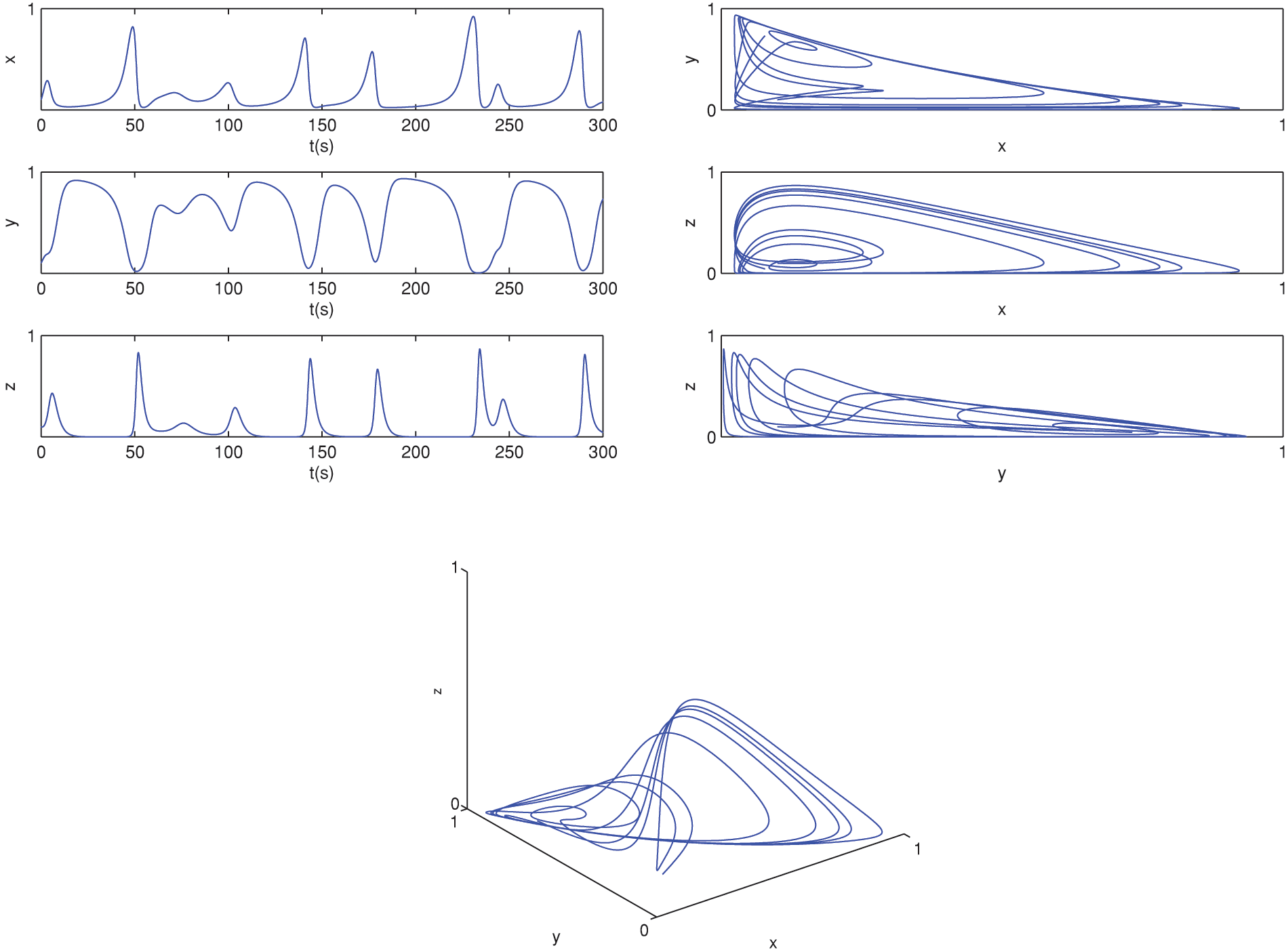
Figure 1: The behavior of the solution at classical derivative

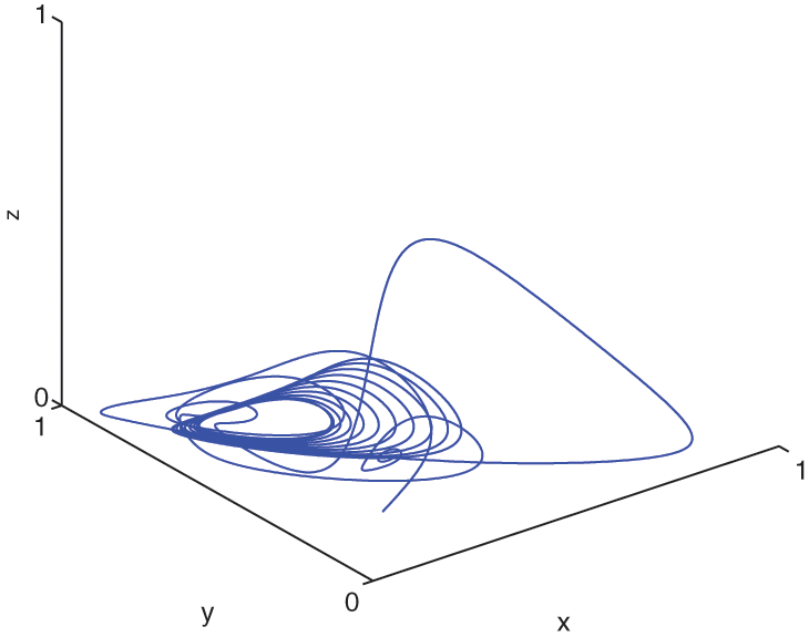
Figure 2: The behavior of the solutions for (6)–(8) at
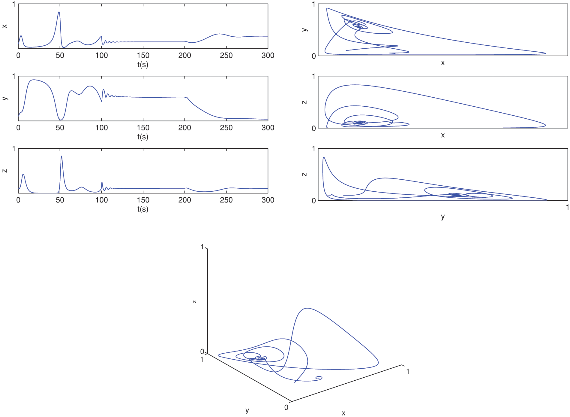
Figure 3: The behavior of the solutions for (6)–(8) at
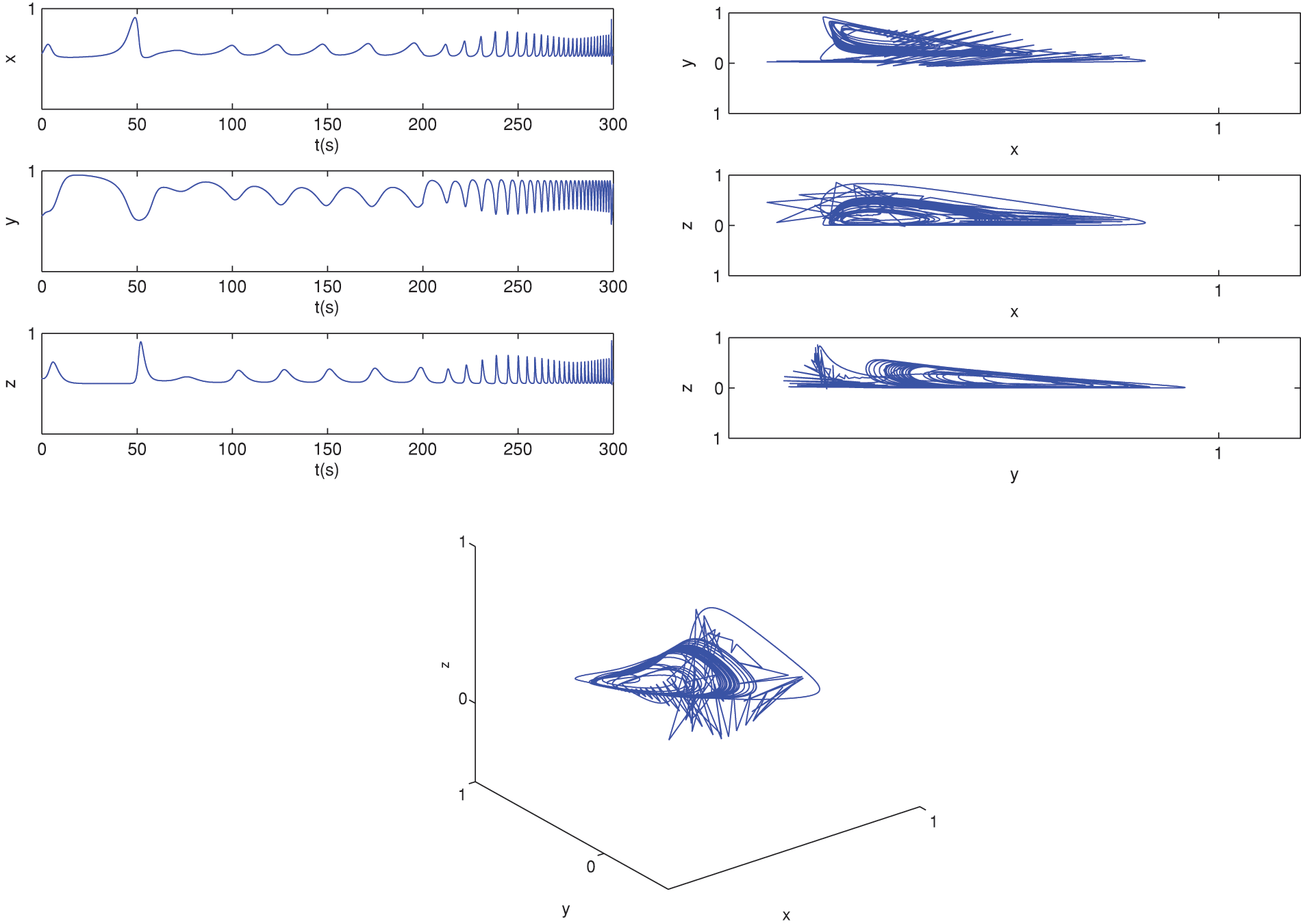
Figure 4: The behavior of the solutions for (6)–(8) at

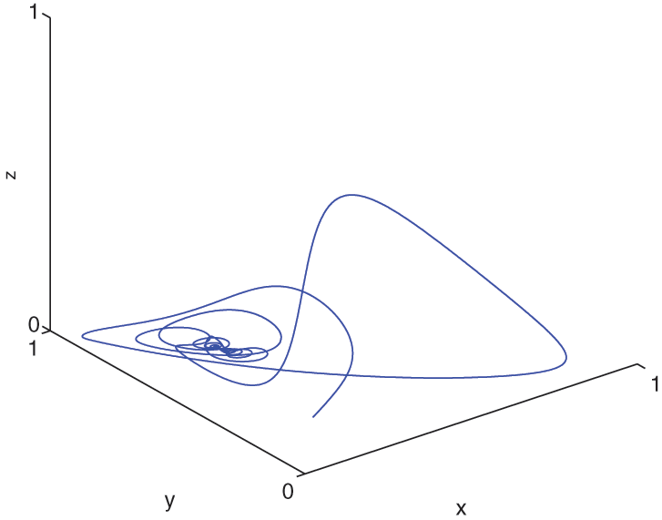
Figure 5: The behavior of the solutions for (6)–(8) at
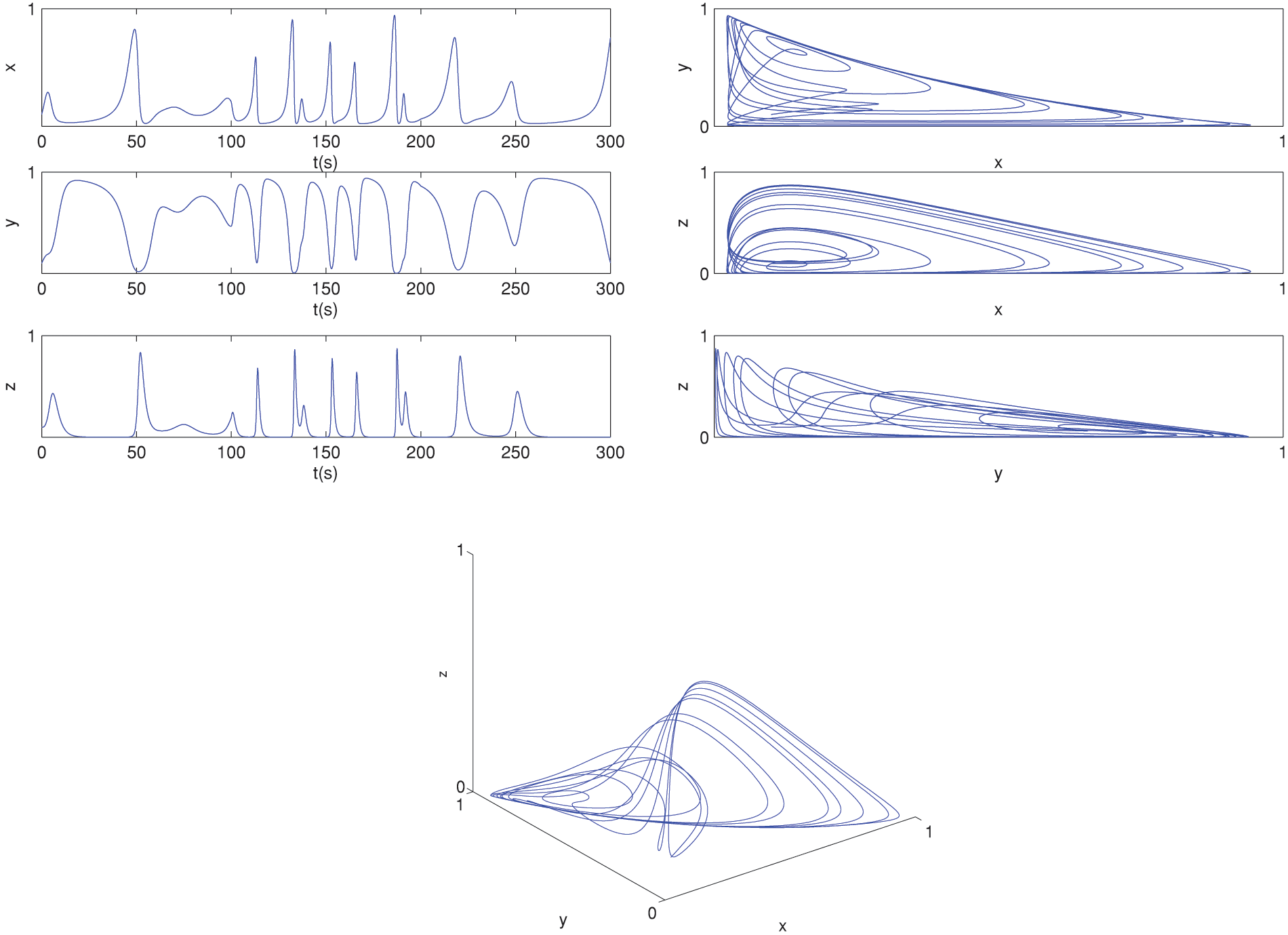
Figure 6: The behavior of the solutions for (6)–(8) at
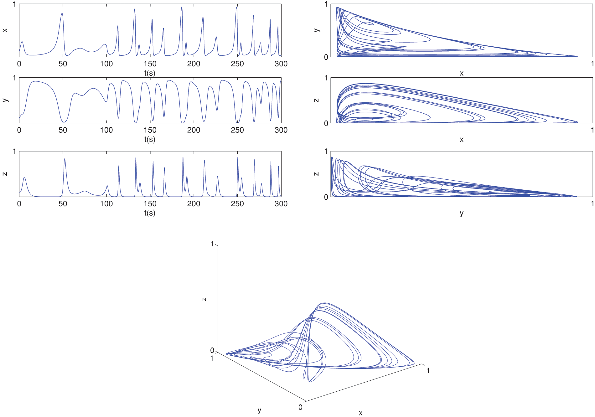
Figure 7: The behavior of the solutions for (6)–(8) at

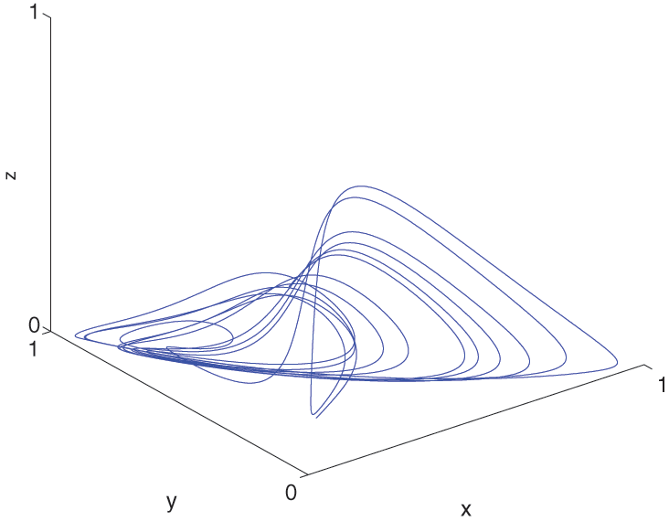
Figure 8: The behavior of the solutions for (9)–(11) at
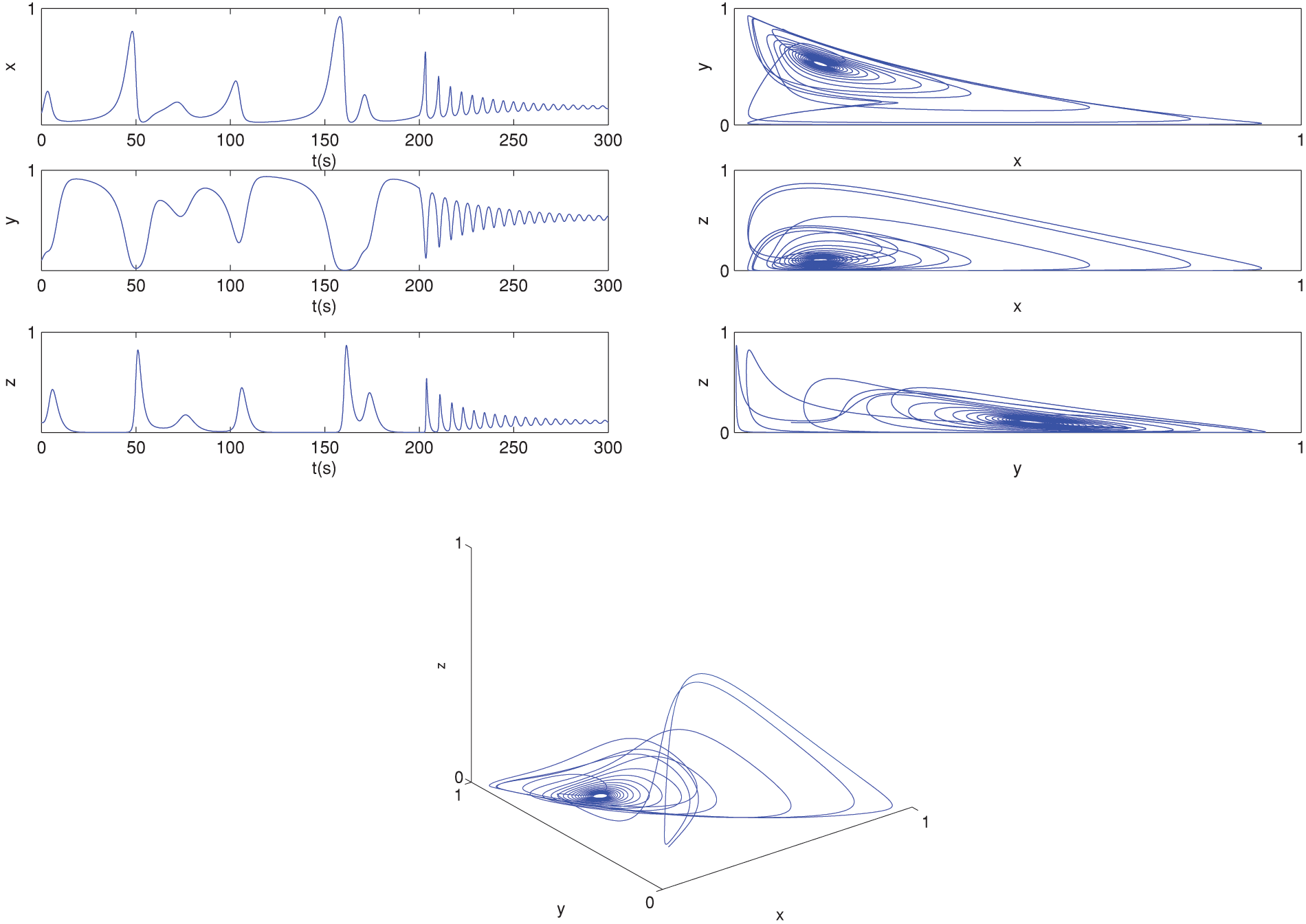
Figure 9: The behavior of the solutions for (9)–(11) at
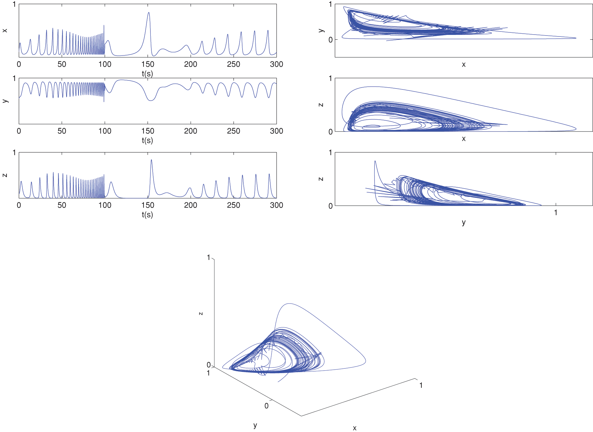
Figure 10: The behavior of the solutions for (9)–(11) at

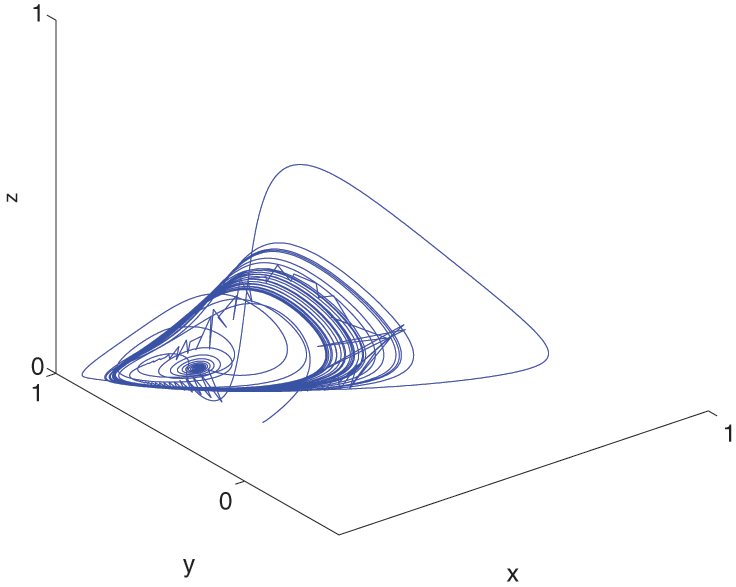
Figure 11: The behavior of the solutions for (9)–(11) at

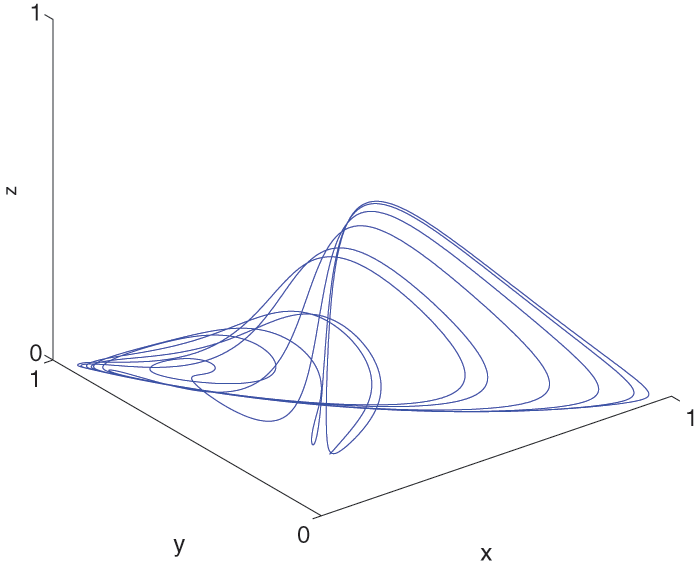
Figure 12: The behavior of the solutions for (9)–(11) at
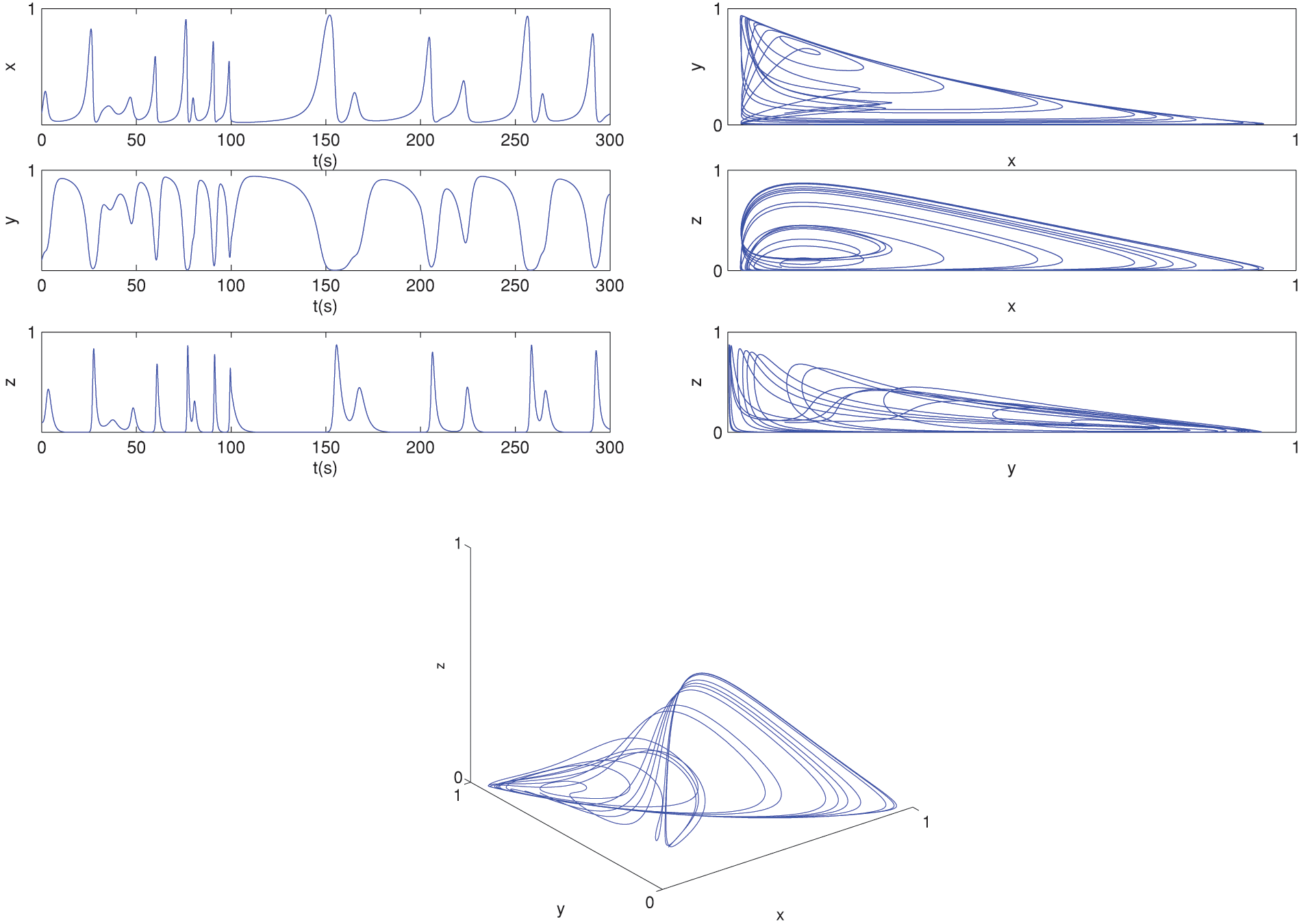
Figure 13: The behavior of the solutions for (9)–(11) at
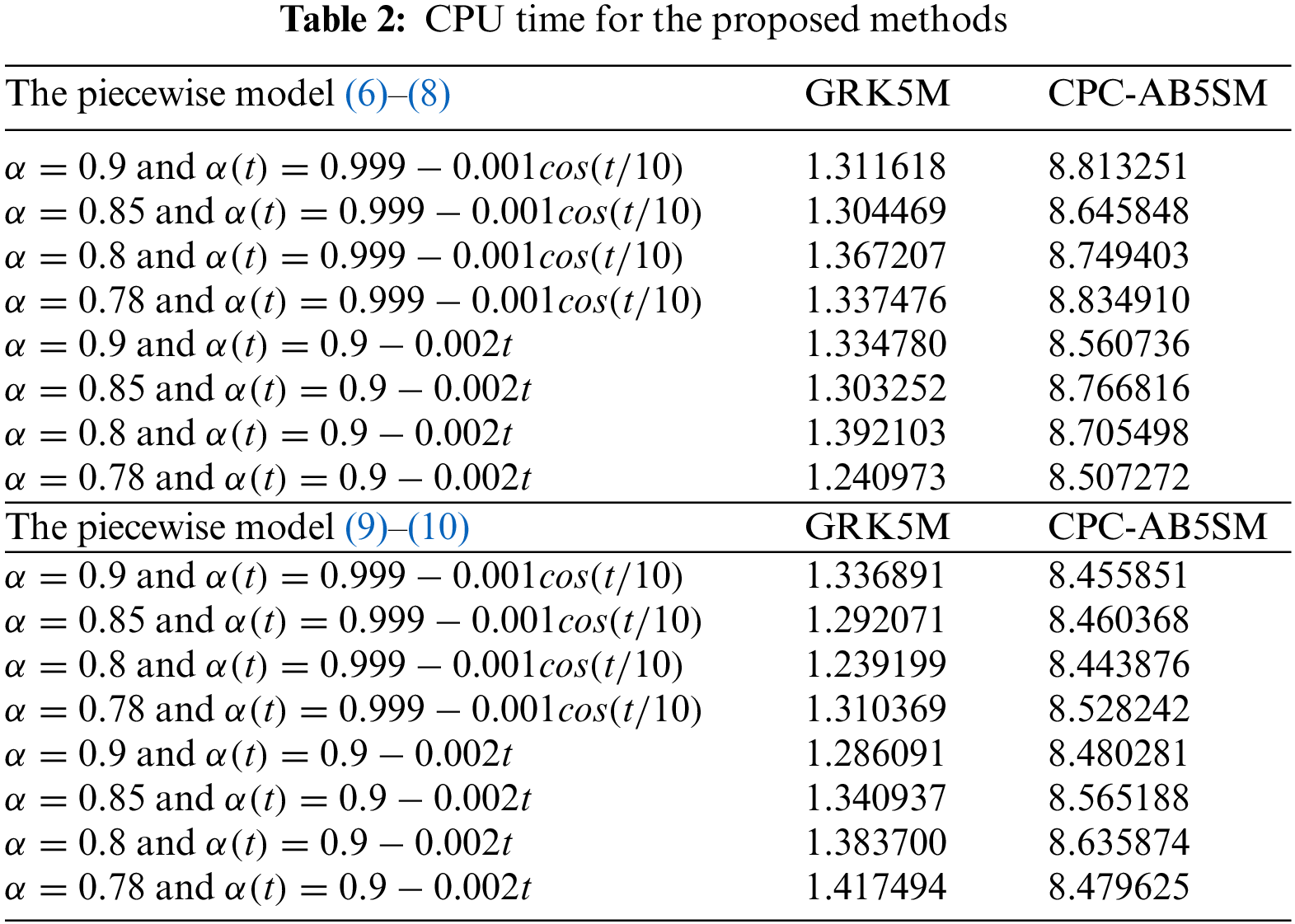
Figs. 1–3 show the behavior of the piecewise model solutions (6)–(8) using CPC-AB5SM (47) with different values of
The behavior of the solutions of the piecewise cancer model Eqs. (6)–(8) using CPC-AB5SM (47) with various values of
Also, Fig. 6 shows the behavior of piecewise model for (6)–(8) using GRK5M (54) at
Figs. 8 and 9 show the behavior of (9) and (10) using CPC-AB5SM (47) and different values of
Fig. 12 shows the behavior of (9) and (10) using the GRK5M (54) at
In this manuscript, two new hybrid variable-order fractional piecewise cancer models have been formulated. A detailed analysis of hybrid variable-order fractional piecewise cancer models is given, where the existence, uniqueness, and stability of the proposed model are established. Caputo proportional constant Adams-Bashfourth fifth step method is constructed with the discretization of the CPC operator to solve the variable-order and fractional order models. The proposed piecewise models are numerically studied using CPC-AB5SM and GRK5M. New behaviors were presented by numerical simulations for the proposed models. Through a series of numerical tests, we have showcased the efficiency of the proposed method and garnered robust empirical support for our theoretical findings. From the obtained simulation, the proposed method is better than the GRK5M in solving such models. We conclude from the results that the piecewise mathematical model representation of cancer in this study has exposed a property that has never been considered or observed in earlier studies using mathematical models based on classical, different fractional derivatives and variable order fractional derivatives. This approach of piecewise mathematical model representation of different real-world dynamic systems is an eye-opener for researchers as the approach has the potential to uncover hidden properties in the dynamics of a system. In the future, the present study can be extended to optimal control problems. In the future, we will extend this study to more complex dynamical systems.
Acknowledgement: The authors wish to express sincere appreciation to the reviewers for their valuable comments, which significantly improved this paper.
Funding Statement: This study did not receive any funding in any form.
Author Contributions: The authors confirm their contribution to the paper as follows: study conception and design: Nasser Sweilam, Seham M. Al-Mekhlafi; data collection: Aya Ahmed, Seham M. Al-Mekhlafi; analysis and interpretation of results: Nasser Sweilam, Seham M. Al-Mekhlafi; draft manuscript preparation: Aya Ahmed, Emad Abo-Eldahab, Ahoud Alsheri, Seham M. Al-Mekhlafi. All authors reviewed the results and approved the final version of the manuscript.
Availability of Data and Materials: The data that support the findings of this study are available from the first and corresponding authors upon reasonable request.
Conflicts of Interest: The authors declare that they have no conflicts of interest to report regarding the present study.
References
1. Kuznetsov, V. A., Knott, GD. (2001). Modeling tumor regrowth and immunotherapy. Mathematical and Computer Modelling, 33(12–13), 1275–1287. [Google Scholar]
2. de Pillis, L. G., Radunskaya, A. (2003). The dynamics of an optimally controlled tumor model: A case study. Mathematical and Computer Modelling, 37(11), 1221–1244. https://doi.org/10.1016/S0895-7177(03)00133-X [Google Scholar] [CrossRef]
3. Jahanshahi, H., Shanazari, K., Mesrizadeh, M., Soradi-Zeid, S. (2020). Numerical analysis of galerkin meshless method for parabolic equations of tumor angiogenesis problem. The European Physical Journal Plus, 135(11), 1–23. [Google Scholar]
4. Attia, R. A. M., Tian, J., Lu, D., Aguilar, J. F. G. (2022). Unstable novel and accurate soliton wave solutions of the nonlinear biological population model. Arab Journal of Basic and Applied Sciences, 29(1), 19–25. https://doi.org/10.1080/25765299.2021.2024652 [Google Scholar] [CrossRef]
5. Syam, M. I., Al-Refai, M., Fractional differential equations with Atangana-Baleanu fractional derivative: Analysis and applications. Chaos, Solitons & Fractals, 2, 100013. https://doi.org/10.1016/j.csfx.2019.100013 [Google Scholar] [CrossRef]
6. Sweilam, N. H., AL-Mekhlafi, S. M., Baleanu, D. (2021). A hybrid stochastic fractional order coronavirus (2019-nCov) mathematical model. Chaos, Solitons & Fractals, 145, 110762. https://doi.org/10.1016/j.chaos.2021.110762 [Google Scholar] [PubMed] [CrossRef]
7. Sweilam, N. H., Al-Ajami, T. M. (2015). Legendre spectral-collocation method for solving some types of fractional optimal control problems. Journal of Advanced Research, 6(3), 393–403. https://doi.org/10.1016/j.jare.2014.05.004 [Google Scholar] [PubMed] [CrossRef]
8. Baleanu, D., Fernandez, A., Akg, A. (2020). On a fractional operator combining proportional and classical differ-integrals. Mathematics, 8(3),360. https://doi.org/10.3390/math8030360 [Google Scholar] [CrossRef]
9. Kumar, S., Chauhan, R. P., Momani, S., Hadid, S. (2020). Numerical investigations on COVID-19 model through singular and nonsingular fractional operators. Numerical Methods for Partial Differential Equations, 1–27. https://doi.org/10.1002/num.22707 [Google Scholar] [CrossRef]
10. Safare, K. M., Betageri, V. S., Prakasha, D. G., Veeresha, P., Kumar, S. (2020). A mathematical analysis of ongoing outbreak COVID-19 in India through nonsingular derivative. Numerical Methods for Partial Differential Equations, 37(2), 1282–1298. [Google Scholar]
11. Khan, M. A., Atangana, A., Alzahrani, E., Fatmawati (2020). The dynamics of COVID-19 with quarantined and isolation. Advances in Difference Equations, 2020, 425. https://doi.org/10.1186/s13662-020-02882-9 [Google Scholar] [PubMed] [CrossRef]
12. Hajipour, M., Jajarmi, A., Baleanu, D. (2018). An efficient nonstandard finite difference scheme for a class of fractional chaotic systems. Journal of Computational and Nonlinear Dynamics, 13(2), 021013.https://doi.org/10.1115/1.4038444 [Google Scholar] [CrossRef]
13. Lin, W. (2007). Global existence theory and chaos control of fractional differential equations. Journal of Mathematical Analysis and Applications, 332(1), 709–726. https://doi.org/10.1016/j.jmaa.2006.10.040 [Google Scholar] [CrossRef]
14. Sweilam, N. H., Al-Mekhlafi, S. M., Albalawi, A. O. (2020). Optimal control for a fractional order malaria transmission dynamics mathematical model. Alexandria Engineering Journal, 59(3), 1677–1692. https://doi.org/10.1016/j.aej.2020.04.020 [Google Scholar] [CrossRef]
15. Omame, A., Abbas, M., Onyenegech, C. P. (2022). Backward bifurcation and optimal control in a co-infection model for SARS-CoV-2 and ZIKV. Results in Physics, 37, 105481.https://doi.org/10.1016/j.rinp.2022.105481 [Google Scholar] [PubMed] [CrossRef]
16. Shah, K., Abdeljawad, T., Ali, A. (2022). Mathematical analysis of the Cauchy type dynamical system under piecewise equations with Caputo fractional derivative. Chaos, Solitons and Fractals, 161(3), 112356. [Google Scholar]
17. Shah, K., Abdeljawad, T., Alrabaiah, H. (2022). On coupled system of drug therapy via piecewise equations. Fractals, 30(8), 114. [Google Scholar]
18. Shah, K., Abdeljawad, T. (2022). Study of a mathematical model of COVID-19 outbreak using some advanced analysis. Waves in Random and Complex Media. https://doi.org/10.1080/17455030.2022.2149890 [Google Scholar] [CrossRef]
19. Shah, K., Abdeljawad, T., Abdalla, B. (2023). Study of fractional order dynamical system of viral infection disease under piecewise derivative. Computer Modeling in Engineering & Sciences, 136(1), 921–941. https://doi.org/10.32604/cmes.2023.025769 [Google Scholar] [CrossRef]
20. Atangana, A., Araz, S. (2021). New concept in calculus: Piecewise differential and integral operators. Chaos, Solitons & Fractals, 145(2), 110638. https://doi.org/10.1016/j.chaos.2020.110638 [Google Scholar] [CrossRef]
21. N’Doye, I., Voos, H., Darouach, M. (2014). Chaos in a fractional-order cancer system. European Control Conference, pp. 171–176. Strasbourg, France. [Google Scholar]
22. Ma, C. Y., Shiri, B., Wu, G. C., Baleanu, D. (2020). New fractional signal smoothing equations with short memory and variable order. Optik, 218. 164507. https://doi.org/10.1016/j.ijleo.2020 [Google Scholar] [CrossRef]
23. Itik, M., Banks, S. P. (2010). Chaos in a three-dimensional cancer model. International Journal of Bifurcation and Chaos, 20(1), 71–79. https://doi.org/10.1142/S0218127410025417 [Google Scholar] [CrossRef]
24. Gómez-Aguilar, J. F., López-López, M. G., Alvarado-Martínez, V. M., Baleanu, D., Khan, H. (2017). Chaos in a cancer model via fractional derivatives with exponential decay and mittag-leffler law. Entropy, 19(12), 681.https://doi.org/10.3390/e19120681 [Google Scholar] [CrossRef]
25. Peinadoa, J., Ibáñez, J., Arias, E., Hernández, V. (2010). Adams-bashforth and adams-moulton methods for solving differential riccati equations. Computers and Mathematics with Applications, 60(11), 3032–3045.https://doi.org/10.1016/j.camwa.2010.10.002 [Google Scholar] [CrossRef]
26. Milici, C., Machado, J. T., Draganescu, G. (2019). Application of the Euler and Runge-kutta generalized methods for FDE and symbolic packages in the analysis of some fractional attractors. International Journal of Nonlinear Sciences and Numerical Simulation, 21(2). https://doi.org/10.1515/ijnsns-2018-0248 [Google Scholar] [CrossRef]
27. Sweilam, N., Al-Mekhlafi, S. M., Shatta, S. A., Baleanu, D. (2022). Numerical treatments for the optimal control of two types variable-order COVID-19 model. Results in Physics, 42, 105964. https://doi.org/10.1016/j.rinp.2022.105964 [Google Scholar] [PubMed] [CrossRef]
Cite This Article
 Copyright © 2024 The Author(s). Published by Tech Science Press.
This work is licensed under a Creative Commons Attribution 4.0 International License , which permits unrestricted use, distribution, and reproduction in any medium, provided the original work is properly cited.


 Submit a Paper
 Propose a Special lssue
 View Full Text
 Download PDF
 Downloads
 Citation Tools