 Open Access
ARTICLE
Prospect Theory Based Individual Irrationality Modelling and Behavior Inducement in Pandemic Control
Department of Automation, BNRist, Tsinghua University, Beijing, 100084, China
* Corresponding Author: H. Vicky Zhao. Email:
Computer Modeling in Engineering & Sciences 2024, 140(1), 139-170. https://doi.org/10.32604/cmes.2024.047156
Received 27 October 2023; Accepted 04 January 2024; Issue published 16 April 2024
Abstract
Understanding and modeling individuals’ behaviors during epidemics is crucial for effective epidemic control. However, existing research ignores the impact of users’ irrationality on decision-making in the epidemic. Meanwhile, existing disease control methods often assume users’ full compliance with measures like mandatory isolation, which does not align with the actual situation. To address these issues, this paper proposes a prospect theory-based framework to model users’ decision-making process in epidemics and analyzes how irrationality affects individuals’ behaviors and epidemic dynamics. According to the analysis results, irrationality tends to prompt conservative behaviors when the infection risk is low but encourages risk-seeking behaviors when the risk is high. Then, this paper proposes a behavior inducement algorithm to guide individuals’ behaviors and control the spread of disease. Simulations and real user tests validate our analysis, and simulation results show that the proposed behavior inducement algorithm can effectively guide individuals’ behavior.Keywords
The outbreak of COVID-19 has led to a severe public health crisis and great economic losses. Governments worldwide have taken various measures, including lockdowns and mandatory quarantines, to inhibit the spread of the disease. However, individuals may not comply with these policies, as many have their own opinions and preferences. In such public health crises, individuals tend to act irrationally, such as excessive panic in an epidemic outbreak and underestimation of the dangers of the epidemics in its later spread, which can significantly affect individuals’ decisions and ultimately affect the spread of the epidemic. Moreover, individuals’ behaviors and the epidemic affect each other. For example, individuals’ behaviors such as social distancing, wearing masks, and isolating can inhibit the spread of the epidemic, and individuals tend to choose protective behaviors when the pandemic is more severe. Therefore, it is crucial to model individuals’ behaviors during the epidemic and determine how to control the spread of the epidemic by guiding individuals’ behaviors without resorting to mandatory measures.
In the following, this paper reviews recent works on epidemic control over networks, individual behavior modeling during an epidemic, and irrational behavior modeling.
There are numerous studies on how to control the epidemic spread over networks, and many attempted to inhibit the epidemic spread on a network by removing nodes. Wang et al. pointed out that the epidemic spread on a network is highly correlated with the largest eigenvalue of the graph’s adjacency matrix [1]. Based on this, existing studies [2–5] attempted to manipulate the adjacency matrix’s eigenvalues by removing nodes to minimize the likelihood of epidemic outbreaks. Meanwhile, some studies [6–8] investigated macro-level approaches to control epidemic spread, such as restricting population movement or implementing proportional quarantine. Besides, studies [9–12] examined the impact of isolation and immunization on disease spread.
The studies on epidemic control investigated how to control the spread by isolating individuals, restricting population movement, etc. However, these studies all assumed that individuals would comply with the control policies, which is usually not the actual situation. In reality, individuals have their own ideas and may not necessarily obey policies such as isolation and movement restrictions.
1.1.2 Individual Behavior Modeling during an Epidemic
Some prior works attempted to model individual behaviors during an epidemic. The studies [13–17] showed that as the proportion of infected individuals in the environment increases, people are more likely to adopt protective behaviors. Zhang et al. assumed that individuals would be more likely to take protective behavior when there is a large proportion of infected neighbors [14], and they analyzed the effect of individual protective behavior on epidemic spread. The model proposed in [15] assumed that an individual’s adoption of protective behavior is affected by the proportion of infected neighbors, as well as regional and global infection rates. The studies [18–20] observed that information dissemination also affects individual protective behavior during the epidemic.
These studies modeled and analyzed individuals’ behavioral choices in the epidemic. However, they did not consider the common and critical issue of individual irrationality, which can significantly affect their decision-making process during an epidemic.
1.1.3 Irrational Behavior Modeling
Individuals usually resort to irrational decision-making when confronted with risks, such as the potential for infection during an epidemic. For instance, many people may be overly panicky in the early stages of an epidemic and may underestimate the risk of the epidemic in the later stages. A challenge here is how to mathematically model such irrational behaviors. Prospect theory provides theoretical models to quantify how individuals tend to overestimate small probabilities and underestimate high probabilities [21–25]. It is crucial to analyze the impact of this irrationality on individuals’ decisions. The study [26] considered risk aversion during the consensus reaching process (CRP) in group decision-making. The studies [27–29] analyzed the impact of irrationality on individuals’ decisions on whether to take vaccination during an epidemic, and they assumed that this is a one-time binary decision problem where users only make one binary decision during the entire epidemic. However, in reality, individuals can take multiple protective behaviors, such as wearing a mask, washing hands, and isolating at home, and they need to continuously decide whether to take such protective behaviors and which behavior to take during the entire epidemic. Individuals may choose to adopt the highest-level protective measures such as self-isolation when the epidemic is rapidly spreading, and choose to not take any protective behaviors when the epidemic is declining.
The existing studies modeled individuals’ irrationality and simple decisions such as whether to take a vaccination. However, they did not consider the continuous interaction and mutual influence between the epidemic spread and individual choices over time in the context of irrational behaviors.
Our work differs from prior works in two aspects. First, prior works on individual behavior modeling in epidemics either ignore the impact of irrational decision-making or fail to consider the continuous interaction and mutual influence between the epidemic spread and individual behaviors. In this paper, the prospect theory is applied to model individuals’ irrational decisions during an epidemic and the co-evolution of individuals’ behaviors and the epidemic. We theoretically analyze the impact of the individuals’ irrationality on their decisions as well as the epidemic. Second, existing works on epidemic control assume individuals’ absolute compliance with the government’s policies such as mandatory isolation. In this paper, based on the individual behavioral model, we propose an effective method to guide individuals’ behaviors and control the epidemic spread. In contrast to prior approaches, our disease spread control method does not rely on mandatory measures.
The main contributions of our work are:
• We build an M-choice epidemic-behavior co-evolution model to simulate individuals’ irrational decision-making and analyze their impact on the epidemic. We theoretically analyze the co-evolution of user behavior and epidemic and its steady state. Also, the impact of irrationality on individuals’ behaviors and disease spread is theoretically analyzed.
• Given the above individual behavior model, we propose a behavior inducement algorithm to guide individuals’ decisions to control the epidemic.
• We validate our individual behavior model and behavior inducement algorithm through simulations. In addition, we use real user tests to validate the conclusions about the impact of irrationality on individuals’ behavior.
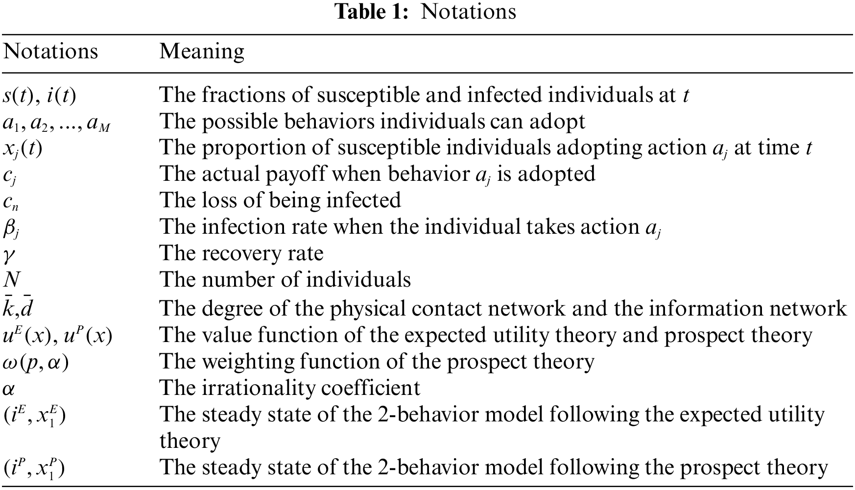
The rest of the paper is organized as follows. Section 2 introduces our proposed epidemic-behavior co-evolution model. Section 3 analyzes the steady state of the epidemic-behavior dynamics and the influence of irrationality. Section 4 presents the behavior inducement method to control the disease spread. Section 5 provides the simulation results. Section 6 shows the results of real user tests, and conclusions are given in Section 8. The important notations of this paper are listed in Table 1.
2 The M-Choice Epidemic-Behavior Co-Evolution Model
During an epidemic, individual behavioral choices and the spread of the disease mutually influence each other. When the probability of infection and the potential losses are high, people tend to adopt protective behaviors, which in turn can inhibit the epidemic spread. In this section, we propose a model to capture the co-evolution of individual behavioral choices and disease spread during a pandemic. We consider irrational behavior in our model and use the model with rational behavior assumption as a baseline to analyze the impact of irrationality on the evolutionary dynamics of the epidemic and its steady states. Based on the model presented in [30], we assume that individuals have a choice among M possible behaviors based on the severity of the epidemic, and these behavioral choices, in turn, affect the epidemic spread.
Following the work in [19], two undirected networks are used in this paper to represent the connections among individuals. The first network is the physical contact network where the disease spreads. The second network is the information network where individuals exchange information about their current health state and behavioral choices. It is worth noting that the two networks are different. In reality, an individual may get infected by strangers in a restaurant or on a bus, while their behaviors will not be influenced by these strangers since they have not interacted with them. Similarly, individuals’ decisions may be influenced by their friends on the Internet without any physical contact with each other. To simplify the analysis, we make the assumption that both the physical contact network and the information network are regular networks consisting of N nodes, where each node represents an individual. In a regular network, each node has a fixed degree, denoted as
Our model consists of two interconnected parts: the disease spread model and the behavior change model. The disease spread model quantifies how the epidemic spreads through the network given the current behaviors of all individuals, and the behavior change model describes how individuals update their behaviors based on the current number of infected individuals and the behaviors of their neighbors. The illustration of our model is in Fig. 1. In the following, the two components of our model will be introduced in detail.
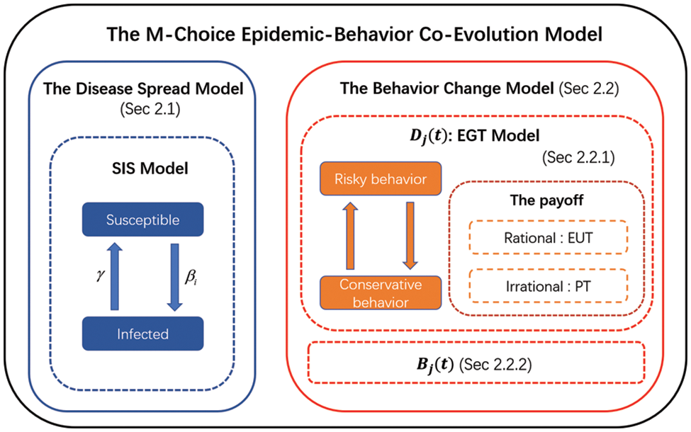
Figure 1: The proposed M-choice epidemic-behavior co-evolution model
We use the classic Susceptible-Infected-Susceptible (SIS) model to depict disease spread, which describes the disease spread process using differential equations. In addition to depicting disease spread, this method of differential equations has a wide range of applications, such as describing the spread of viruses in the body [31,32] and the evolution of opinions [33,34]. In the SIS model, each individual can be in one of two health states: susceptible or infected. We divide time into slots of equal length. At each time slot, a susceptible individual can be infected by an infected individual at a certain infection rate, and an infected individual recovers at a certain recovery rate. We assume that susceptible individuals can adopt different protective measures to reduce their risk of infection, and they have a total of M possible behavioral options
where
The individual behavior model quantifies the dynamics of
In Section 2.2.1, we focus on modeling
Game theory models strategic interactions among agents, providing insights into decision-making across diverse scenarios, from social networks [35] to supply chains [36] and beyond. To model individuals’ active behavior changes in response to their neighbors’ impact and the proportion of infected individuals, we employ the evolutionary game theory, which is a useful framework to investigate the impact of neighbors on individuals’ decisions [37,38]. The basic elements of the evolutionary game theory include individual, strategy, payoff, and strategy update rules. These elements will be introduced one by one in the following.
Individual and Strategy: Each individual is represented as a node in the information network. As mentioned in Section 2.1, we assume that there are a total of M possible protective behaviors
The Payoff: In this paper, we study the protective behavior of susceptible individuals. Note that infected individuals have different health states from susceptible ones, and they adopt the same and fixed strategy of no protective behaviors. Therefore, in this work, we assume that susceptible individuals do not value these infected individuals’ decisions, and the strategies of all susceptible individuals are only affected by their susceptible neighbors. So we define the payoff for susceptible individuals only, and ignore the payoffs of infected individuals, as they do not affect susceptible individuals’ update of their strategies.
In each time slot, every susceptible individual receives a payoff determined by the chosen strategy and interactions with neighbors. In this paper, we consider two scenarios where the susceptible individual is rational and irrational. Therefore, we define the payoff of different behaviors based on the expected utility theory (EUT) [39] and prospect theory (PT) [23], respectively, where EUT models the individual as a rational person and PT considers the individual’s irrationality. Here, following the prior work in [29], to simplify the analysis, we assume that either all individuals are rational or they are all irrational, and compare the two results to analyze the impact of users’ irrationality on the co-evolution of individuals’ behaviors and the epidemic.
Rational individuals’ payoff function: Expected utility theory (EUT) is an economic theory that models the decision-making of rational individuals. When an individual chooses a specific behavior, denoted as
In our behavior modeling and epidemic control problem, every susceptible individual adopting protective behavior
Irrational individuals’ payoff function: Different from the expected utility theory (EUT), the prospect theory (PT) considers the irrational tendencies exhibited by individuals when faced with uncertainty. In PT, individuals tend to overestimate the probability of small risks and underestimate the probability of large risks [21]. Therefore, not only are the actual and the perceived payoffs different, but the actual and the perceived probabilities are also different when irrational individuals face uncertainties.
Similar to EUT, the value function
where
In addition, instead of using the actual probability
where
Given the probability weighting function in (7) and the value function
In our problem, same as the analysis of
Note that if the value functions of EUT and PT are identical (i.e.,
Strategy Update Rules: In each time unit,
where
In our work, we assume that individuals with different behaviors are uniformly distributed in the entire network. Therefore, the probability that the focal individual
where
Combining (10) and (12), we have
In reality, even if individuals do not change their behaviors, the proportion of susceptible individuals with different behaviors will change over time due to transitions in health states. Let
Note that
Given (14), (15) and
2.2.3 The Overall Behavior Change Dynamics
Combining (3), (13) and (16), the complete differential equations describing the dynamics of individual behavior change are
2.3 The Dynamics and the Steady States of the Epidemic-Behavior Co-Evolution Model
Based on the disease spread Eq. (2) and the behavior change dynamics (17), the M-choice epidemic-behavior co-evolution model is obtained as follows:
Here, the first differential equation represents the dynamics of individuals’ health states, and the subsequent M equations model the changes in the proportions of susceptible individuals choosing each of the M behaviors.
At the steady state, both the proportion of infected individuals
To find the steady state of our M-choice disease spread and behavior change model, we follow an approach that is similar to [46] and apply Lyapunov’s first method [47].
Definition 1. The steady-state
where
and
3 Analysis of the Steady State and the Influence of Irrationality for the 2-Behavior Model
To obtain insights into the co-evolution process of epidemic spread and behavioral choice and their steady states, in this section, we consider a simple scenario where each susceptible individual can take two possible behaviors and the theoretical solution of (19) can be obtained. For example, a susceptible individual may either choose risky behavior such as continuing to go out in spite of the epidemic, or choose conservative behavior such as home isolation. Home isolation can significantly reduce the risk of being infected, but it leads to substantial economic loss and affects people’s physical and mental well-being. During the epidemic, individuals need to choose between high-cost low-risk conservative behavior and low-cost high-risk risky behavior. Their decisions are often influenced by the severity of the epidemic and the potential loss due to home isolation. People tend to choose self-isolation when the epidemic poses a greater threat to their health, and they tend to go out when the loss due to home isolation is too high (e.g., losing their jobs and income). By investigating this simple scenario, this paper aims to gain insights into the co-evolution process and its steady states, and theoretically analyze the impact of irrationality on the epidemic as well as individuals’ behaviors. For the more general scenario with more than two possible behavior choices, we use numerical solutions and simulation results to show the evolution process, and an example with three possible behavior choices is provided in Appendix A in Supplementary Material.
In this section, based on our model in the previous section, we analyze the evolution of the epidemic and the dynamics of individuals’ choices between two behaviors: the risky behavior (going out) represented by
3.1.1 The Steady States with All Rational Individuals
When all individuals are rational, the payoff is modeled by EUT in (5). Since
where
Theorem 1. The steady state
where
When
Proof: See Appendix B in Supplementary Material.
From Theorem 1, there are three possible steady states, which correspond to three different situations in reality:
• Case 1: The steady state
• Case 2: For the steady state
• Case 3: The steady state
3.1.2 The Steady States with Irrational Individuals
Next, we consider the scenario where all individuals are “irrational”, and model their payoff function using the PT. By substituting the PT utility function (9) into (17), the dynamic of the epidemic and the behavior can be expressed as:
Similarly, we can get the steady state of (23) in Theorem 2.
Theorem 2. The steady state
When
Proof: See Appendix D in Supplementary Material.
The three stable states in PT are similar to those in EUT:
• Case 1: The steady state (0,1) is the same as Case 1 under EUT. In this situation, the epidemic will always die out, and all individuals will choose the risky behavior.
• Case 2: The steady state
• Case 3: The steady state
3.2 Analysis of Individuals’ Irrationality
In this section, we analyze the influence of individuals’ irrationality on the steady state. In the weighting function in (7), the irrationality coefficient quantifies the irrationality degree of individuals, and a smaller value of
Theorem 3. Given the same set of system parameters (
3a. When
3b. When
If
– When
– When
On the contrary, if
– When
– When
3c. When
– In addition, if
– On the contrary, if
Proof: See Appendix E in Supplementary Material.
To better understand Theorem 3, note that in (24), Case 1 represents the situation where the infection rate is too low and the epidemic will eventually die out no matter how individuals choose their behaviors. Therefore, individuals’ irrationality will not affect the outcome when
For Theorem 3b, when
For Theorem 3c, when
Note that from Section 2.2, if the value functions of EUT and PT are identical (i.e.,
In summary, irrationality tends to make individuals become more extreme, that is, risk-averse when the risk is small and risk-seeking when the risk is high.
4 Behavior Inducement to Control the Disease Spread
In this section, based on our previous analysis in Sections 2 and 3, we study how to guide individuals’ behaviors and control epidemic spread through policy design and develop effective behavior inducement algorithms.
4.1 The Optimal Behavior Inducement Algorithms
We first discuss measures that governments can take to guide individuals’ behaviors during an epidemic. For example, they can incentivize or penalize certain behaviors, such as subsidizing risky behaviors (e.g., going out) to boost the economy, penalizing risky behaviors, or encouraging conservative behaviors (such as staying at home and wearing masks) to control the disease spread. In our model, this means the parameters
Next, we discuss the goals of behavior guidance. The first goal is to control the spread of the disease at the steady state. For example, the government may wish to keep the number of infected people as low as possible. Here, the loss caused by the epidemic is represented as
Since the irrationality coefficient should fall within
In this work, we do not specify the specific forms of
and the same constraint also holds for
From (24), there are three possible steady states. To solve the optimization problem (27), we need to consider all three possible steady states and analyze the optimal solution for each, which is very complicated. Then we introduce Theorem 4 to simplify this problem.
Given the system parameters and
where
From our analysis in Appendix F in Supplementary Material, we have the following Theorem 4.
Theorem 4. For the optimization problem (27), if
• if
• If
• If
From Theorem 4, we only need to model and solve the problem for Case 3 in (24), which greatly reduces the complexity of our problem.
4.2 Solving the Optimization Problems
In this section, we consider the following scenario and use it as an example to demonstrate how to model and solve the optimization problem in (27). Consider the scenario where the government wants to control epidemic spread and reduce its impact on the economy and people’s mental health. It means that, at the steady state after behavior inducement
Since the infection rate
From Theorem 4, we only need to get the optimal solution in Case 3 and then we can get the optimal solution of the whole space by comparing it with
Note that in (30),
Fig. 2 presents two examples of the feasible region of (
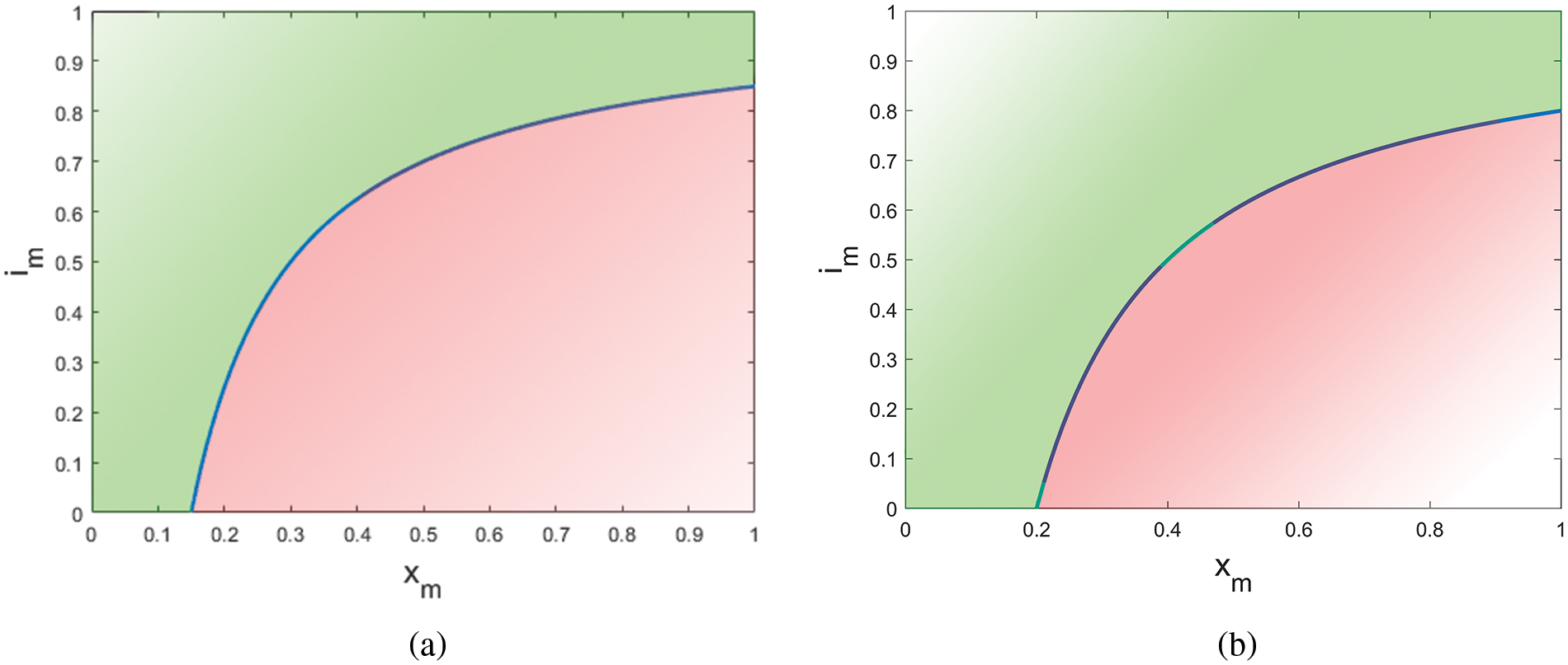
Figure 2: The range of
4.2.2 Solving the Optimization Problem with Feasible Constraints
If
where
According to Theorem 4, the optimization problem can be transformed into the problem in Case 3 and then we can get the optimal solution of the whole space by comparing it with
Here,
4.2.3 Reformulation of the Optimization Problem When the Constraints Are Infeasible
If the constraints
We can use the same method in Section 4.2.2 to solve (34), and the details are provided in Appendix H in Supplementary Material.
In this section, we first run simulations to validate our steady state analysis of the co-evolution process and the effect of irrationality on individuals’ behaviors and epidemic spread in Section 3. Then we validate the effectiveness of the behavior guidance algorithms proposed in Section 4. As there are few previous works have analyzed how to model irrational individuals in a pandemic, we do not compare our method with other works in this section.
5.1 Simulations of the Steady States of EUT and PT
Theorem 1 and Theorem 2 give theoretical analyses of the steady states when individuals are rational and irrational, respectively. To validate the two theorems, as an example, we conducted simulations on regular networks with 500 nodes. The physical contact network has a fixed degree of 10, while the information network has a degree of 20. We observe similar trends on other types of networks and with other parameters. We set the recovery rate to
Fig. 3 shows the simulation and theoretical results of
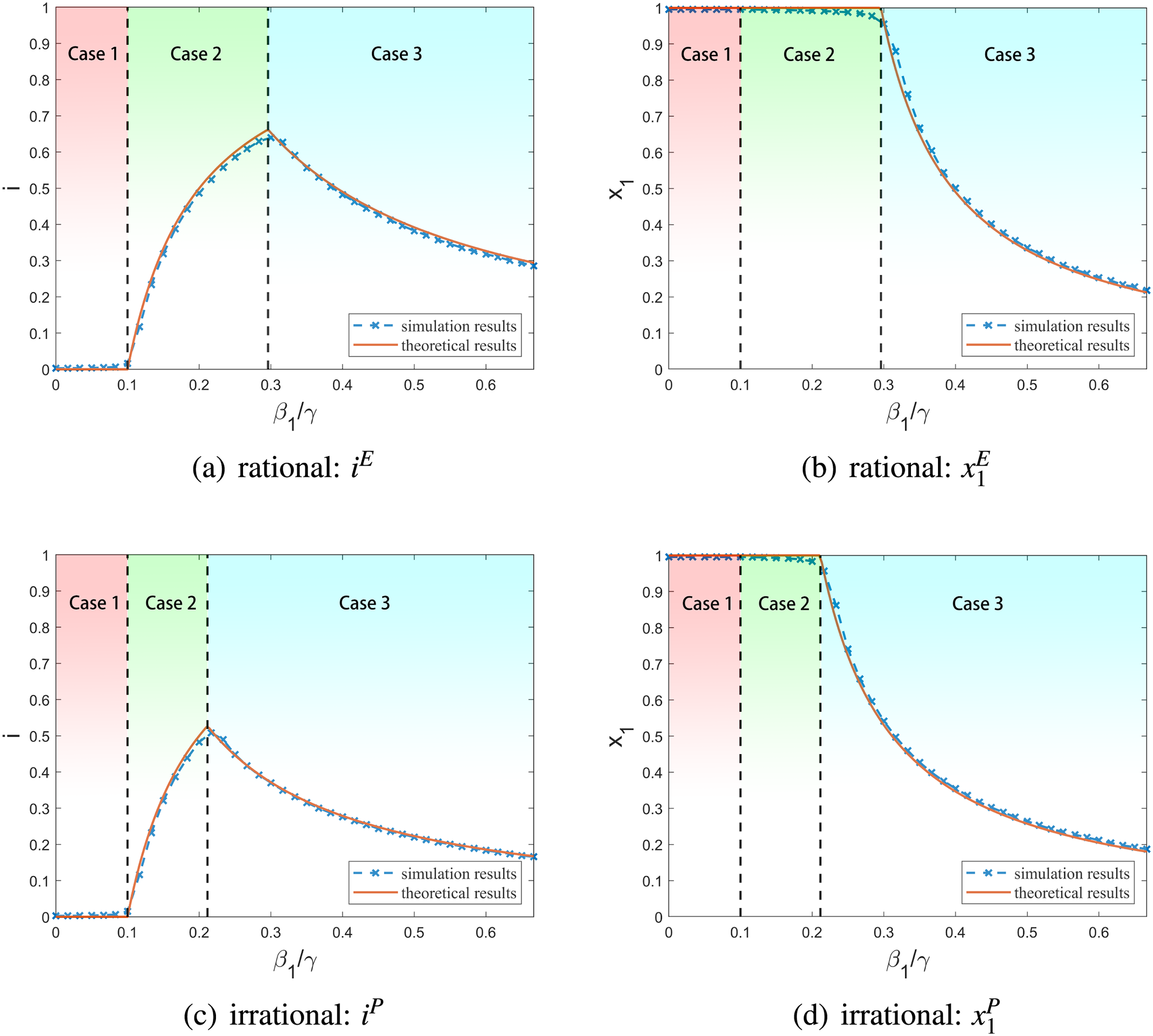
Figure 3: Simulation results of the steady states with rational and irrational individuals
Then we validate Theorem 3 and investigate the impact of irrationality on the steady states using the same simulation setup as before. Fig. 4 shows the average results of 50 simulation runs. We observe the same trend for other types of networks and other parameter settings. Note that in Fig. 4,
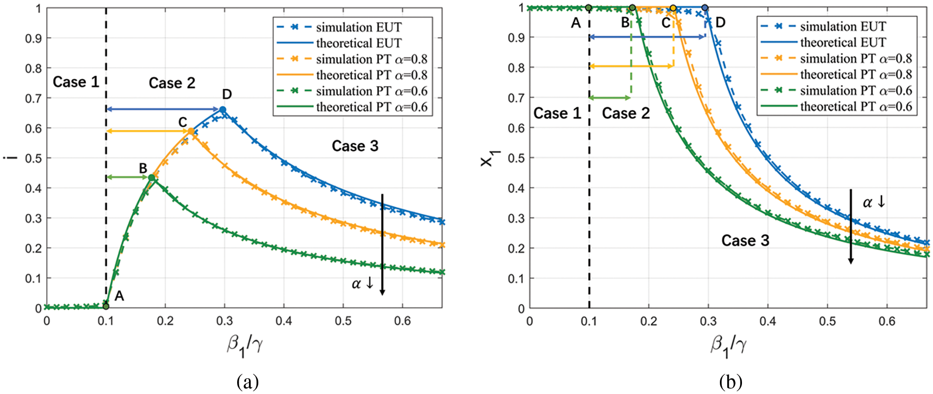
Figure 4: Simulation results of the steady states with different
• Before Point A, i.e., when
• Between Points A and B,
• Between Points B and C,
• After Point C,
The above shows an example where irrationality promotes conservative behaviors, and in most parameter settings, irrationality makes individuals more conservative. Appendix I in Supplementary Material shows an example where irrationality makes individuals risk-seeking. This situation only occurs when the infection rate is high, and the loss of disease is extremely low.
In summary, the simulation results effectively validate our analysis in Theorem 3.
5.2 Simulations of the Behavior Inducement Algorithm
Then we simulate the behavior inducement algorithm proposed in Section 4. We run simulations on regular networks with 500 nodes and a fixed degree of 10 for both the physical contact network and the information network. We let
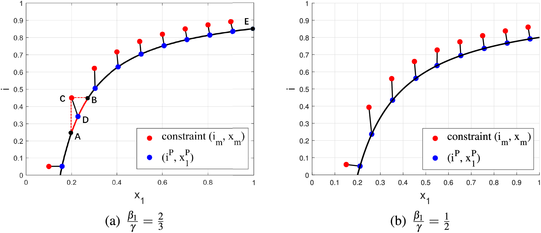
Figure 5: Simulation results of behavior inducement algorithm with feasible constraints
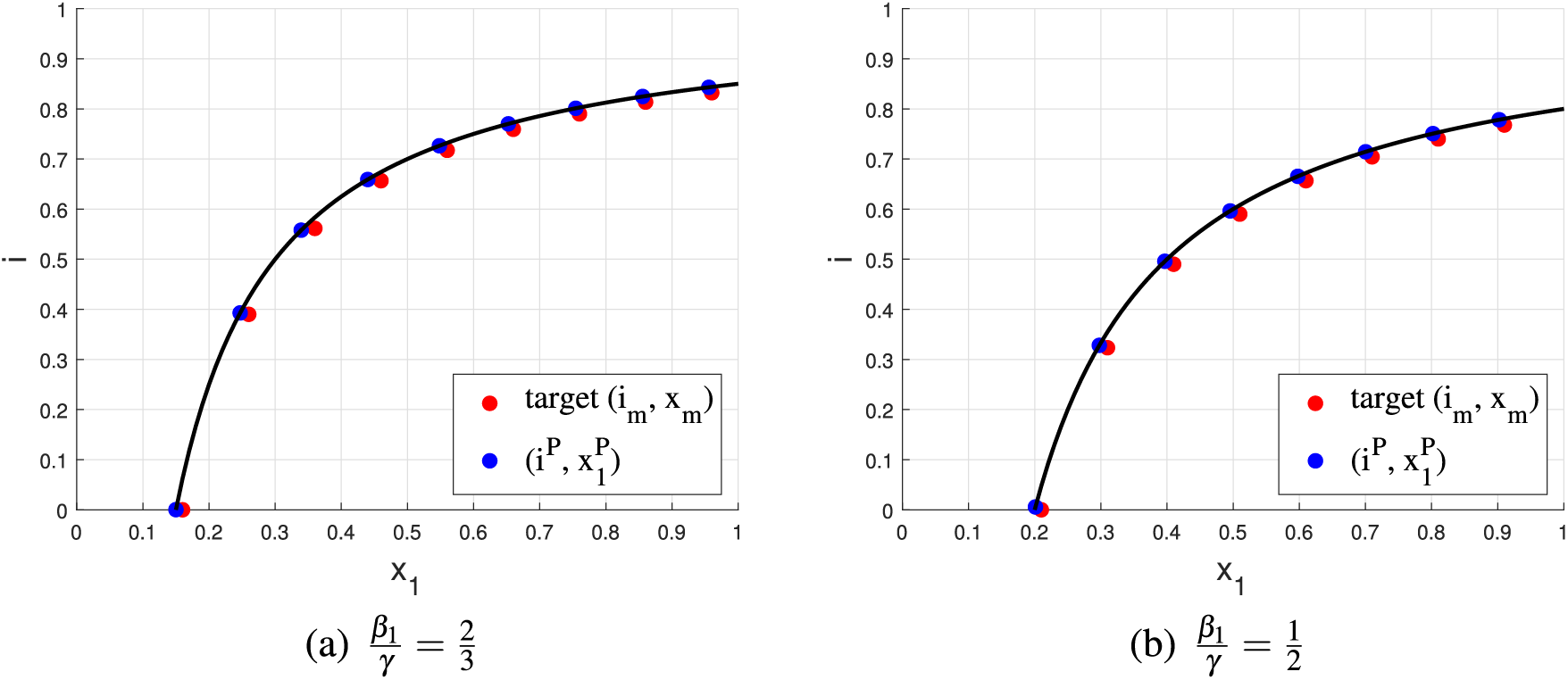
Figure 6: Simulation results of the behavior inducement algorithm with infeasible constraints
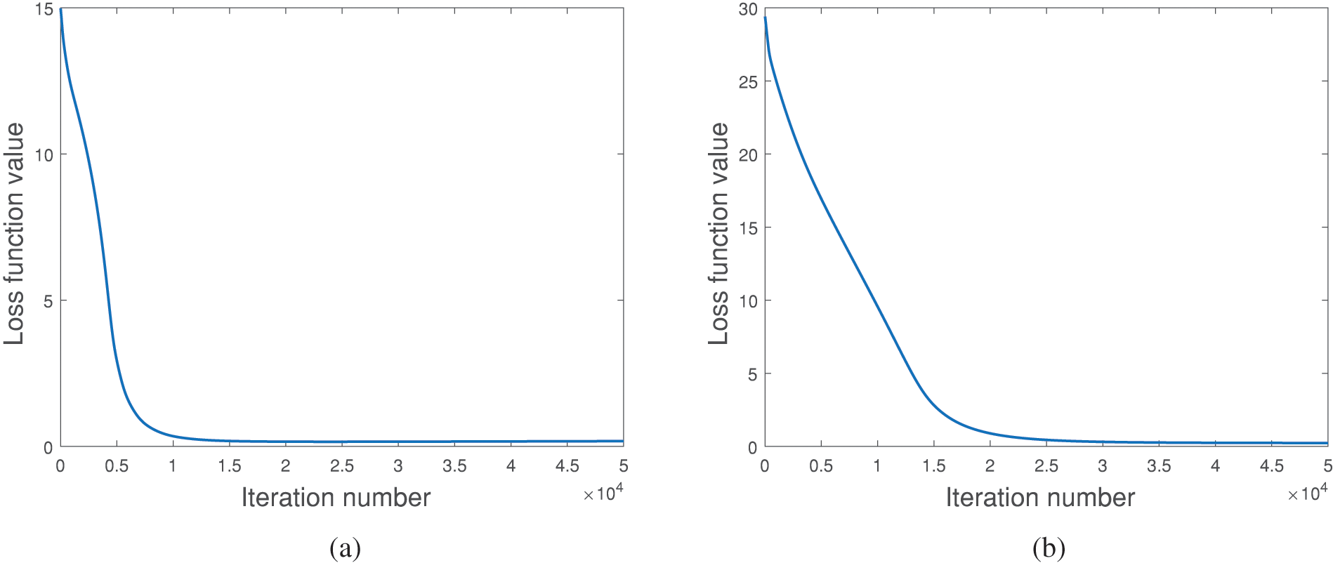
Figure 7: Simulation results of the behavior inducement algorithms. (a) The loss function in (33) with feasible constraints, and (b) the loss function in (34) with infeasible constraints
The results of the proposed algorithm under feasible constraints are shown in Fig. 5. The black solid line represents the boundary between the feasible and infeasible regions;
Simulation results of the proposed behavior inducement algorithm with infeasible constraints are shown in Fig. 6. Here, the given two constraints (
In summary, from Fig. 5–7, our behavior inducement algorithm is effective and converges well.
While the simulation experiments have validated our theoretical analysis, it is necessary to further validate our conclusions using real user tests. However, obtaining real user data on behavioral choices, network structure, and spread data simultaneously poses a significant challenge. Therefore, we qualitatively validate our conclusions through sociological experiments. In our test, 550 subjects were interviewed, including 237 males and 313 females. The distribution of data is provided in Appendix J in Supplementary Material.
In our test, we first collect data to estimate the irrationality coefficient
6.1 Estimating the Irrationality Coefficient
Data collection:Following the works in [23–25], we estimate the subjects’ irrationality coefficient
Question A: You have a
a. When the price is lower than
b. When the price is lower than
c. When the price is lower than
d. When the price is lower than
e. When the price is lower than
f. Even if the price is higher than
After the subjects have made their initial choices, a refined set of choices is presented to them to obtain fine-grained results. For instance, if a subject chooses option
Estimation of
Similar to [25], we use (7) and (6) as the probability weighting function and the value function, respectively, in our work. Note that from the definitions, we have
which is equivalent to
In (37),
6.2 Measuring Individuals’ Risk Preference
Data Collection: Then we proceed to collect data on the behavioral choices of different subjects when confronted with risky scenarios during a pandemic. In each question of this section, subjects are presented with a specific epidemic situation. Within each scenario, subjects must choose between going out and staying at home. They are informed that if they choose to go out, there is a certain probability of becoming infected. If they decide to stay at home, they are guaranteed not to be infected, but they will suffer from some form of loss. Below is an example in our experiment.
Question B: There is an epidemic spreading right now. If you come into contact with an infected person, you have a 5% probability of being infected. If you choose to go out, you will be in close contact with 20 people every day. If you decide to stay at home, you are guaranteed not infected but will suffer from some losses. However, if you go out, there is a chance of becoming infected. The loss of being infected is 20 times that of the loss due to home isolation. Your city has a population of 1 million, then:
a. When there is no confirmed case in the city, I will go out.
b. When the number of confirmed cases in the city is less than 10, I will go out.
c. When the number of confirmed cases in the city is less than 100, I will go out.
d. When the number of confirmed cases in the city is less than 1,000, I will go out.
e. When the number of confirmed cases in the city is less than 10,000, I will go out.
f. When the number of confirmed cases in the city is less than 100,000, I will go out.
g. When the number of confirmed cases in the city is higher than 100,000, I will still go out.
Calculating Individuals’ Risk Preference
6.3 Analysis of the Relationship between Irrationality and Behavioral Choice
We classify subjects into different groups based on their irrationality coefficient
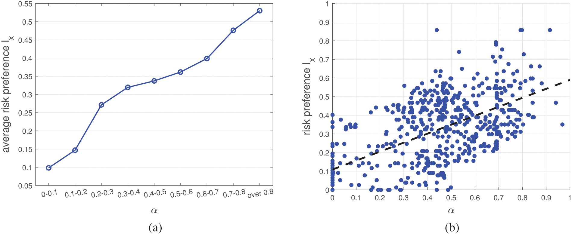
Figure 8: (a) The relationship between
Moreover, we also plot scatter plots of
7.1 The Impact of Cultural and Social Elements
Cultural and social elements can influence individual behavioral choices and disease spread, and our model can be used to analyze them to a certain extent.
First, in reality, an individual’s understanding and views of an epidemic may be affected by culture, beliefs, and social environment. For example, people in different countries have different opinions about COVID-19 [52]. Moreover, political opinions will also affect individuals’ concerns about COVID-19 [53]. In our model, people with different cultures and political opinions can have different
In addition, different costs of implementing policies in different cultures and countries can be reflected in our behavior inducement algorithm. For example, in some countries or cultures, the cost of implementing policies is lower, and individuals are more inclined to obey behavioral inducement. In our model, that means they have a lower
7.2 The Implementation of Behavior Inducement Method
In Section 4, we discuss how to control the spread of disease through behavior inducement. We assume that individuals’
Change people’s understanding of the diseases: Propaganda can influence people’s awareness of the dangers of diseases. For example, during the COVID-19 crisis, there was a tendency among supporters of the US Democratic Party to perceive COVID-19 as more harmful compared to supporters of the Republican Party. This disparity largely stemmed from the propaganda policies employed by the two parties [53]. Therefore, individuals’
Reward or punish specific behaviors: Governments can guide people’s behavior by rewarding and punishing specific behaviors. For example, reward the behavior of staying at home or punish the behavior of going out to control the spread of the disease. In this approach, an individual’s
Change people’s irrationality coefficient: Propaganda via social networks and media can influence individuals’ irrationality [49]. For example, the government can publicize during the disease that people do not need to overestimate the probability of small events and do not need to panic too much, which could reduce the irrationality of individuals. Then individuals’
Through theoretical analysis and experiments, we get some insights into disease spread control, which can guide government policies to a certain extent.
First, considering the practicalities of governance, the government can employ a multifaceted approach to control spread, utilizing methods like incentivizing and penalizing behaviors and raising awareness about the disease through propaganda. Through our experiments, we observe that the efficacy of a singular measure diminishes as its intensity increases. Therefore, employing multiple measures simultaneously can yield superior outcomes at a reduced cost.
Second, the influence of irrationality has great significance. The degree of individual irrationality can be affected by propaganda and other means. Through experiments, we find that changing the irrational coefficient
Finally, as discussed in Section 4.2, there are limits to the two goals of controlling spread and reducing economic losses. Therefore, governments need to formulate reasonable policies and make a trade-off between controlling the spread of disease and reducing economic losses. For example, in the case of certain seasonal and highly detrimental diseases, the government may opt to maximize control measures to limit the spread, even if it will lead to substantial short-term economic losses. In the case of prolonged epidemic diseases, it becomes crucial to pay increased attention to the long-term economic loss.
In this paper, we propose an epidemic-behavior co-evolution framework to analyze the co-evolution of user behavior and the disease spread during an epidemic. Our model considers the irrationality of individuals’ decision-making processes, and our theoretical analysis shows that individual irrationality polarizes individual behavior choices. That is, irrationality makes users risk-averse when the probability of being infected is small, while they tend to be risk-seeking when the probability of being infected is large. We then propose a behavior inducement algorithm to control the disease spread and reduce losses by guiding individual behavior. Simulation results show the correctness of our theoretical analysis and verify the validity of our guidance control method. We also qualitatively prove the correctness of our conclusions using real-user tests. Different from the prior works, in this work, we use prospect theory to model the individuals’ irrational behaviors during an epidemic and the co-evolution of individuals’ behaviors and the epidemic. Our research contributes to comprehending the irrational behavioral choices made by individuals during epidemics. Additionally, our behavior inducement approach does not rely on mandatory policies like prior works, providing a viable framework for governments to effectively control disease spread during epidemics.
Acknowledgement: None.
Funding Statement: The authors received no specific funding for this study.
Author Contributions: Wenxiang Dong built the model, derived the theory, conducted simulations and real user tests, and wrote the paper. H. Vicky Zhao provided research guidance and edited the paper.
Availability of Data and Materials: In our ethics application for the real user tests, we promised to protect the privacy of all test subjects. Therefore, we cannot provide the specific data of each sample in the real user tests. The distribution of the data can be provided upon request.
Conflicts of Interest: The authors declare that they have no conflicts of interest to report regarding the present study.
Supplementary Materials: The supplementary material is available online at https://doi.org/10.32604/cmes.2024.047156.
1We consider those epidemics with
2Note that from (21), if
3If
References
1. Wang, Y., Chakrabarti, D., Wang, C., Faloutsos, C. (2003). Epidemic spreading in real networks: An eigenvalue viewpoint. 22nd International Symposium on Reliable Distributed Systems, Florence, Italy, IEEE. [Google Scholar]
2. Tong, H., Prakash, B. A., Tsourakakis, C., Eliassi-Rad, T., Faloutsos, C. et al. (2010). On the vulnerability of large graphs. 2010 IEEE International Conference on Data Mining, Sydney, Australia, IEEE. [Google Scholar]
3. Chen, C., Tong, H., Prakash, B. A., Tsourakakis, C. E., Eliassi-Rad, T. et al. (2015). Node immunization on large graphs: Theory and algorithms. IEEE Transactions on Knowledge and Data Engineering, 28(1), 113–126. [Google Scholar]
4. Ahmad, M., Tariq, J., Shabbir, M., Khan, I. (2017). Spectral methods for immunization of large networks. Australasian Journal of Information Systems, 21, 1563. [Google Scholar]
5. Saxena, C., Doja, M., Ahmad, T. (2018). Group based centrality for immunization of complex networks. Physica A: Statistical Mechanics and its Applications, 508, 35–47. [Google Scholar]
6. Birge, J. R., Candogan, O., Feng, Y. (2022). Controlling epidemic spread: Reducing economic losses with targeted closures. Management Science, 68(5), 3175–3195. [Google Scholar]
7. Wan, R., Zhang, X., Song, R. (2021). Multi-objective model-based reinforcement learning for infectious disease control. Proceedings of the 27th ACM SIGKDD Conference on Knowledge Discovery & Data Mining, New York, USA, ACM. [Google Scholar]
8. Hota, A., Godbole, J., Pare, P. (2021). A closed-loop framework for inference, prediction, and control of sir epidemics on networks. IEEE Transactions on Network Science and Engineering, 8(3), 2262–2278. [Google Scholar]
9. Alazman, I., Albalawi, K. S., Goswami, P., Malik, K. (2023). A restricted sir model with vaccination effect for the epidemic outbreaks concerning COVID-19. Computer Modeling in Engineering & Sciences, 137(3), 841–854. https://doi.org/10.32604/cmes.2023.028674 [Google Scholar] [CrossRef]
10. Chen, Z., Zha, H., Shu, Z., Ye, J., Pan, J. (2022). Assess medical screening and isolation measures based on numerical method for COVID-19 epidemic model in japan. Computer Modeling in Engineering & Sciences, 130(2), 841–854. https://doi.org/10.32604/cmes.2022.017574 [Google Scholar] [CrossRef]
11. Farman, M., Akgül, A., Ahmad, A., Baleanu, D., Umer Saleem, M. (2021). Dynamical transmission of coronavirus model with analysis and simulation. Computer Modeling in Engineering & Sciences, 127(2), 753–769. https://doi.org/10.32604/cmes.2021.014882 [Google Scholar] [CrossRef]
12. Chu, Y. M., Sultana, S., Rashid, S., Alharthi, M. S. (2023). Dynamical analysis of the stochastic COVID-19 model using piecewise differential equation technique. Computer Modeling in Engineering & Sciences, 137(3), 2427–2464. [Google Scholar]
13. Xu, Y. H., Wang, H. J., Lu, Z. W., Hu, M. B. (2023). Impact of awareness dissemination on epidemic reaction–diffusion in multiplex networks. Physica A: Statistical Mechanics and its Applications, 621, 128723. [Google Scholar]
14. Zhang, H. F., Xie, J. R., Tang, M., Lai, Y. C. (2014). Suppression of epidemic spreading in complex networks by local information based behavioral responses. Chaos, 24(4), 043106. [Google Scholar]
15. Wu, Q., Fu, X., Small, M., Xu, X. J. (2012). The impact of awareness on epidemic spreading in networks. Chaos, 22(1), 013101. [Google Scholar] [PubMed]
16. Bagnoli, F., Lio, P., Sguanci, L. (2007). Risk perception in epidemic modeling. Physical Review E, 76(6), 061904. [Google Scholar]
17. Shang, Y. (2013). Modeling epidemic spread with awareness and heterogeneous transmission rates in networks. Journal of Biological Physics, 39(3), 489–500. [Google Scholar] [PubMed]
18. Funka, S., Gilada, E., Watkinsb, C., Jansena, V. A. (2009). The spread of awareness and its impact on epidemic outbreaks. Proceedings of the National Academy of Sciences of the United States of America, 106(16), 6872–6877. [Google Scholar] [PubMed]
19. Granell, C., Gómez, S., Arenas, A. (2013). Dynamical interplay between awareness and epidemic spreading in multiplex networks. Physical Review Letters, 111(12), 128701. [Google Scholar] [PubMed]
20. Granell, C., Gómez, S., Arenas, A. (2014). Competing spreading processes on multiplex networks: Awareness and epidemics. Physical Review E, 90(1), 012808. [Google Scholar]
21. Kahneman, D., Tversky, A. (2013). Prospect theory: An analysis of decision under risk. In: Handbook of the fundamentals of financial decision making: Part I, pp. 99–127. Hackensack, NJ, USA: World Scientific. [Google Scholar]
22. Prelec, D. (1998). The probability weighting function. Econometrica, 66(3), 497–527. [Google Scholar]
23. Tversky, A., Kahneman, D. (1992). Advances in prospect theory: Cumulative representation of uncertainty. Journal of Risk and Uncertainty, 5(4), 297–323. [Google Scholar]
24. Gonzalez, R., Wu, G. (1999). On the shape of the probability weighting function. Cognitive Psychology, 38(1), 129–166. [Google Scholar] [PubMed]
25. Prelec, D. (2000). Compound invariant weighting functions in prospect theory, pp. 67–92. Cambridge, UK: Cambridge University Press Cambridge. [Google Scholar]
26. Ji, Y., Ma, Y. (2023). The robust maximum expert consensus model with risk aversion. Information Fusion, 101866. [Google Scholar]
27. Oraby, T., Bauch, C. T. (2015). Bounded rationality alters the dynamics of paediatric immunization acceptance. Scientific Reports, 5(1), 10724. [Google Scholar] [PubMed]
28. Hota, A. R., Sundaram, S. (2019). Game-theoretic vaccination against networked sis epidemics and impacts of human decision-making. IEEE Transactions on Control of Network Systems, 6(4), 1461–1472. [Google Scholar]
29. Li, X. J., Li, X. (2020). Perception effect in evolutionary vaccination game under prospect-theoretic approach. IEEE Transactions on Computational Social Systems, 7(2), 329–338. [Google Scholar]
30. Poletti, P., Caprile, B., Ajelli, M., Pugliese, A., Merler, S. (2009). Spontaneous behavioural changes in response to epidemics. Journal of Theoretical Biology, 260(1), 31–40. [Google Scholar] [PubMed]
31. Attaullah, Ramzi, D., Weera, W. (2022). Galerkin time discretization scheme for the transmission dynamics of hiv infection with non-linear supply rate. AIMS Mathematics, 6, 11292–11310. [Google Scholar]
32. Attaullah, Alyobi, S., Yassen, M. F. (2022). A study on the transmission and dynamical behavior of an hiv/aids epidemic model with a cure rate. AIMS Mathematics, 7(9), 17507–17528. [Google Scholar]
33. Wang, L., Schuetz, C. G., Cai, D. (2021). Choosing response strategies in social media crisis communication: An evolutionary game theory perspective. Information & Management, 58(6), 103371. [Google Scholar]
34. Wang, J., Wang, X., Fu, L. (2020). Evolutionary game model of public opinion information propagation in online social networks. IEEE Access, 8, 127732–127747. [Google Scholar]
35. Molinero, X., Riquelme, F. (2021). Influence decision models: From cooperative game theory to social network analysis. Computer Science Review, 39, 100343. [Google Scholar]
36. Li, S., Qu, S. (2023). The three-level supply chain finance collaboration under blockchain: Income sharing with shapley value cooperative game. Sustainability, 15(6), 5367. [Google Scholar]
37. Jiang, C., Chen, Y., Liu, K. R. (2014). Graphical evolutionary game for information diffusion over social networks. IEEE Journal of Selected Topics in Signal Processing, 8(4), 524–536. [Google Scholar]
38. Li, Y., Zhao, H. V., Chen, Y. (2022). Graphical evolutionary game theoretic modeling of strategy evolution over heterogeneous networks. IEEE Transactions on Signal and Information Processing over Networks, 8, 739–754. [Google Scholar]
39. Simon, H. A. (1955). A behavioral model of rational choice. The Quarterly Journal of Economics, 69(1), 99–118. [Google Scholar]
40. Wakker, P. P. (2010). Prospect theory: For risk and ambiguity. Cambridge, UK: Cambridge University Press. [Google Scholar]
41. Kephart, J. O., White, S. R. (1992). Directed-graph epidemiological models of computer viruses. In: Computation: The micro and the macro view, pp. 71–102. Hackensack, NJ, USA: World Scientific. [Google Scholar]
42. Wu, J. T., Leung, K., Leung, G. M. (2020). Nowcasting and forecasting the potential domestic and international spread of the 2019-nCoV outbreak originating in Wuhan, China: A modelling study. The Lancet, 395(10225), 689–697. [Google Scholar]
43. Zhu, S., Srebric, J., Spengler, J. D., Demokritou, P. (2012). An advanced numerical model for the assessment of airborne transmission of influenza in bus microenvironments. Building and Environment, 47, 67–75. [Google Scholar] [PubMed]
44. Foster, A., Kinzel, M. (2021). Estimating COVID-19 exposure in a classroom setting: A comparison between mathematical and numerical models. Physics of Fluids, 33(2), 021904. [Google Scholar] [PubMed]
45. Traulsen, A., Claussen, J. C., Hauert, C. (2004). Coevolutionary dynamics: From finite to infinite populations. Physical Review Letters, 95(23), 238701. [Google Scholar]
46. Karlsson, C. J., Rowlett, J. (2020). Decisions and disease: A mechanism for the evolution of cooperation. Scientific Reports, 10(1), 13113. [Google Scholar] [PubMed]
47. Lyapunov, A. M. (1992). The general problem of the stability of motion. International Journal of Control, 55(3), 531–534. [Google Scholar]
48. Chakrabarti, D., Wang, Y., Wang, C., Leskovec, J., Faloutsos, C. (2008). Epidemic thresholds in real networks. ACM Transaction on Information and System Security, 10(4), 1–26. [Google Scholar]
49. Toczyski, P., Banerski, G. (2021). Patterns of digital users’ irrationality in the moment of digital transformation of the media. In: Digital interaction and machine intelligence, pp. 115–124. Springer International Publishing. [Google Scholar]
50. Gogtay, N. J., Thatte, U. M. (2017). Principles of correlation analysis. Journal of the Association of Physicians of India, 65(3), 78–81. [Google Scholar]
51. Senthilnathan, S. (2019). Usefulness of correlation analysis. SSRN Electronic Journal. https://doi.org/10.2139/ssrn.3416918 [Google Scholar] [CrossRef]
52. Dryhurst, S., Schneider, C. R., Kerr, J., Freeman, A. L., Recchia, G. et al. (2022). Risk perceptions of covid-19 around the world. In: COVID-19, pp. 162–174. London, UK: Routledge. [Google Scholar]
53. Bruine de Bruin, W., Saw, H. W., Goldman, D. P. (2020). Political polarization in us residents’ COVID-19 risk perceptions, policy preferences, and protective behaviors. Journal of Risk and Uncertainty, 61, 177–194. [Google Scholar] [PubMed]
Cite This Article
 Copyright © 2024 The Author(s). Published by Tech Science Press.
This work is licensed under a Creative Commons Attribution 4.0 International License , which permits unrestricted use, distribution, and reproduction in any medium, provided the original work is properly cited.


 Submit a Paper
 Propose a Special lssue
 View Full Text
 Download PDF
 Downloads
 Citation Tools