Comparative Analysis of ARIMA and LSTM Model-Based Anomaly Detection for Unannotated Structural Health Monitoring Data in an Immersed Tunnel

1  Introduction

To prevent the structural performance deterioration-induced catastrophic failures of immersed tunnel, the establishment of a Structural Health Monitoring (SHM) system has emerged as an effective solution [1–5]. A pivotal role of the SHM system is to monitor performance data and issue structural warnings through anomaly detection [6]. Traditionally, tunnel operators have relied on empirical judgment or simplistic fixed alarm thresholds to determine maintenance actions [7–10]. However, this fixed threshold approach either missed alarms or suffered from frequent false alarms. The approach failed because of its oversimplification of the problem as the long-term transformation of tunnel structures and the potential of vast SHM data were not considered.

The rapidly advancing digital transformation in infrastructure has thrust data-driven anomaly detection methods into the research spotlight. Autoregressive Support Vector Machines, as proposed in [11], outperform linear models by integrating sensor outputs for effective damage identification. Principal Component Analysis has enhanced long-term tunnel SHM [12], effectively detecting subtle deviations for potential early warning systems. The Switching Kalman Filter method [13] excels in identifying anomalies in structural behavior, demonstrating precision in detecting dam anomalies. Real-time anomaly detection using Bayesian Dynamic Linear Models [14,15] facilitates continuous parameter learning and efficient anomaly identification. Convolutional Neural Networks (CNN) have been adopted for data preprocessing and anomaly detection [16,17], offering scalability and accuracy. Du et al.’s work [18] introduced CNN-based anomaly detection while addressing class imbalance and limited data. Most recently, Entezami et al. [19] introduced unsupervised meta-learning, effectively addressing data challenges in long-term SHM. Together, these studies have advanced SHM anomaly detection methods, ranging from statistical techniques to cutting-edge deep learning approaches, enhancing accuracy and efficiency in assessing critical infrastructure.

However, for unannotated SHM data, the previously proposed supervised learning approaches have been inadequate due to the algorithms’ inability to learn anomaly patterns with limited examples. Currently, there are only very few studies that combine the mechanism of anomaly patterns with comprehensive data analysis [20–22]. Wang et al.’s studies on settlement characteristics of immersed tunnel and artificial island-immersed tunnel transition areas presented insightful findings and sound analytical results [23,24]. An alternate perspective is to learn normal behaviors by leveraging a substantial number of normal examples, which is the model-based anomaly detection approach discussed in this study. In SHM data, temporal continuity plays a pivotal role in anomaly detection [25]. This implies that data exhibit a high correlation across successive time steps, and sequence patterns tend to change gradually unless an abnormal condition arises. The logic is that if the model can effectively capture the normal behavior patterns within the sequence and understand their dependencies, then the model's predictions should closely align with the actual observations. Consequently, observations deviating significantly from predictions can be flagged as anomalies.

The crux of the model-based anomaly detection approach lies in constructing a prediction model, which falls into two categories. The first category comprises classical time series models such as Autoregressive (AR) model, Moving Average (MA) model, Autoregressive Moving Average (ARMA) model, Autoregressive Integrated Moving Average (ARIMA) model, and Seasonal Autoregressive Integrated Moving Average (SARIMA) model [26]. Capitalizing on temporal continuity, these models capture the temporal dependencies within sequences and provide accurate future predictions. For instance, Zeng et al. [27] proposed an improved m-ARIMA model to detect outliers, successfully reducing warning errors in optical fiber sensors. Liu et al. [28] employed an ARIMA model to predict concrete damage failure in service tunnels due to sulfate erosion. Huang et al. [29] developed an ARIMA model and concluded that it accurately predicted the evolution of tunnel deformational performance in the short term with low computational costs. The ARIMA model, widely applied in engineering, can be synergistically combined with other models for improved predictive capability.

The second category involves deep learning-based time series prediction methods [30]. Among these, Long Short-Term Memory (LSTM) stands out due to its ability to capture long-range temporal dependencies [31]. Li et al. utilized an improved LSTM model to predict acceleration responses in a three-span continuous bridge, utilizing residuals to determine sensor fault thresholds [32]. Son et al. introduced a multilayered LSTM model using tension data from a cable-stayed bridge, classifying abnormal data through reconstruction errors [33]. Dang et al. recognized that each structure possesses unique dynamic properties, and employed a hybrid deep learning architecture featuring CNN and LSTM to extract relevant features from sensory data [34].

Despite these advancements, limited research has systematically compared classical time series models and deep learning models for anomaly detection [35]. Moreover, the majority of research has been focused on large-scale bridges or dams, with limited attention on tunnels [36–38]. Consequently, this paper aims to compare classical ARIMA and deep learning LSTM models for anomaly detection, using the Hong Kong-Zhuhai-Macao Bridge immersed tunnel as a case study. The subsequent sections delineate the methodology (Section 2), present a detailed case study (Section 3), discuss findings (Section 4), and conclude (Section 5).

2  Model-Based Anomaly Detection Approach

2.1 Procedure of Model-Based Anomaly Detection

This section outlines a dynamic model-based approach for anomaly detection. The procedure involves several key steps. Initially, the data collected by the SHM system undergoes preprocessing, which includes format transformation and wavelet threshold denoising. After obtaining standardized and denoised data, a prediction model is constructed using both the ARIMA and LSTM methods. The fundamental concept behind the approach is for the model to capture the normal behavior of the time series. Consequently, if observations deviate significantly from the predictions, indicating a violation of time continuity, they are labeled as anomalies. In essence, if the prediction error falls outside a defined confidence interval, the observation is considered abnormal, leading to the issuance of hierarchical warning signals based on the degree of deviation. The flow chart of the procedure is depicted in Fig. 1.

Figure 1: Flow chart of the model-based anomaly detection approach

It is noteworthy that the method employs a rolling single-step prediction, continually advancing the time window while incorporating new observations into the model input. However, as time progresses, the model parameters need updating as the initial model fitted to previous data becomes less suitable for accurate predictions. Updating the model at every second is impractical due to time constraints. Thus, the paper introduces two metrics to govern when model updates occur: average deviation size and duration of model use. These metrics dictate parameter updates if the average error over a recent period exceeds an acceptable threshold or if the time interval since the last update surpasses a predefined maximum. This approach is based on the assumption that the presence of relatively few anomalies allows for their deviations to minimally impact subsequent model predictions. Additionally, incorporating time control acknowledges the evolving nature of the model over time.

Moreover, the confidence interval for prediction results should be tailored to the external environment and tunnel structure. Drawing inspiration from the PauTa Criterion or 3σ rule, the threshold can be determined based on historical data within a specific period. This statistical approach requires a sufficiently lengthy historical reference period to ensure a roughly normal distribution of sample data. However, the chosen period should not be excessively long, as a fixed threshold is only accurate under stable conditions. Based on the results of repeated attempts and considering that the dynamic prediction model updates this threshold to a reasonable range, this study adopts the statistical results of 1 h of SHM data to calculate the initial threshold value. However, it should be noted that this statistical-based threshold-setting approach may be influenced by data distribution skewness or overly stable conditions. Further studies and validations are needed to establish the optimal threshold-setting methods.

2.2 ARIMA-Based Model

The ARIMA model is a widely used classical time series prediction model, typically denoted as ARIMA (p, d, q), where p signifies the autoregressive parameter reflecting lag observations, d is the number of times that a raw sequence is differenced, and q indicates the moving average parameter denoting the window length. The developments of static and dynamic ARIMA models in this study were the same as those reported by Chen et al. [39].

2.3 LSTM-Based Model

Although classical models like ARIMA excel in time series prediction, their emphasis on linear relationships can constrain the predicted value distribution. Long Short-Term Memory (LSTM) is a widely used artificial neural network for time series modeling. The LSTM model “learns” from historical monitoring sequences and aims to predict the subsequent sequence value. Inputs consist of sequence values within a defined time window, and the goal is to predict the value immediately following the window.

The fundamental structure of LSTM mirrors the Recurrent Neural Network (RNN). The LSTM's distinct feature lies in its capacity to consider not only the current input but also the outputs of previous time steps. This enables the network to retain its previous state and enhances its capacity to learn long-term dependencies within the sequence. The network’s structure, as depicted in Fig. 2, showcases the data flow across time and layers [31–34].

Figure 2: Structure of LSTM

Unlike traditional RNNs, which struggle with long-term dependencies due to vanishing or exploding gradients, LSTM incorporates cell states and gate functions to handle such issues. The forget gate, input gate, and output gate govern the retention or removal of information and cell state modification. The mathematical formulations of these gates and the LSTM unit structure are provided in Eqs. (1)–(6) and Fig. 3 [31–34].

Figure 3: LSTM unit

(1) Forget gate:

Γf=σ(Wf[Xt,ht−1]+bf)(1)

(2) Input gate:

Γi=σ(Wi[Xt,ht−1]+bi)(2)

(3) Output gate:

Γo=σ(Wo[Xt,ht−1]+bo)(3)

(4) Cell state:

ct=tanh⁡(Wc[Xt,ht−1]+bc)(4)

ct=Γi∗ct+Γf∗ct−1(5)

(5) Output value:

ht=Γo∗ct(6)

where σ(x)=11+e−x,tanh=1−e−2x1+e−2x.

In detail, the sigmoid function is used as the activation function for the three gate functions, and the hyperbolic tangent function is used as the activation function for the cell state, which regulates the amount of information obtained. When moving forward from time t−1 to time t, the input of the current time step Xt and the output of the previous time step ht−1 update the cell state ct−1 through the forget gate Γo and input gate Γi. The output ht is then computed based on gate Γo and the updated cell state ct.

As depicted in Fig. 3, giving a more intuitive view of the preceding mathematical formula, where “+” represents matrix addition and “x” represents the dot product. Such a structure enables LSTM to control the retention and abandonment of the information by learning the parameters of the three gates to learn the long-term correlation contained in the sequence.

3  Case Study of an Immersed Tunnel

3.1 Overview of the Investigated Immersed Tunnel and Its SHM Data

The Hong Kong-Zhuhai-Macao Bridge (HZMB), an expansive 55 km-long project spanning Lingdingyang Bay, comprises three integral components: the main project of the bridge, the island, and the undersea tunnel. The information on the undersea immersed tunnel can be obtained from the literature [40,41], and the longitudinal layout of the immersed tunnel is shown in Fig. 4.

Figure 4: Longitudinal layout of the HZMB immersed tunnel

The standard tunnel element is 180 m long, consisting of eight segments each with a length of 22.5 m. The cross-sectional dimensions of the immersed tunnel are shown in Fig. 5.

Figure 5: Cross-sectional dimensions of the HZMB immersed tunnel (unit: mm)

An SHM system has been implemented on the HZMB. The SHM system acquires five types of monitoring data: ground motion, joint deformation, concrete strain, temperature, and humidity, as shown in Table 1. These monitoring items serve the following purposes [42]: (1) Ground motion: it will cause structural vibration or misalignment between the joints. In addition, the HZMB immersed tunnel passes through the sandy soil strata, which may be liquefied under the seismic effect, so special attention should be paid; (2) Strain of elements: important indicator for huge concrete structure; (3) Joint deformation: reflecting the effect and safety reserve of the waterproofing system and the dislocation of the rubber waterstop; (4) Temperature and humidity: reflecting the stress level of the concrete structure and the working environment of the monitoring system. The frequency of data acquisition in the system is 50 Hz.

3.2 Denoising Method

Noise is inevitable in the SHM system because of environmental reasons or unstable installation. Such factors culminate in suboptimal data quality. Fig. 6 presents an enlarged depiction of the concrete strain data before and after the denoising algorithm.

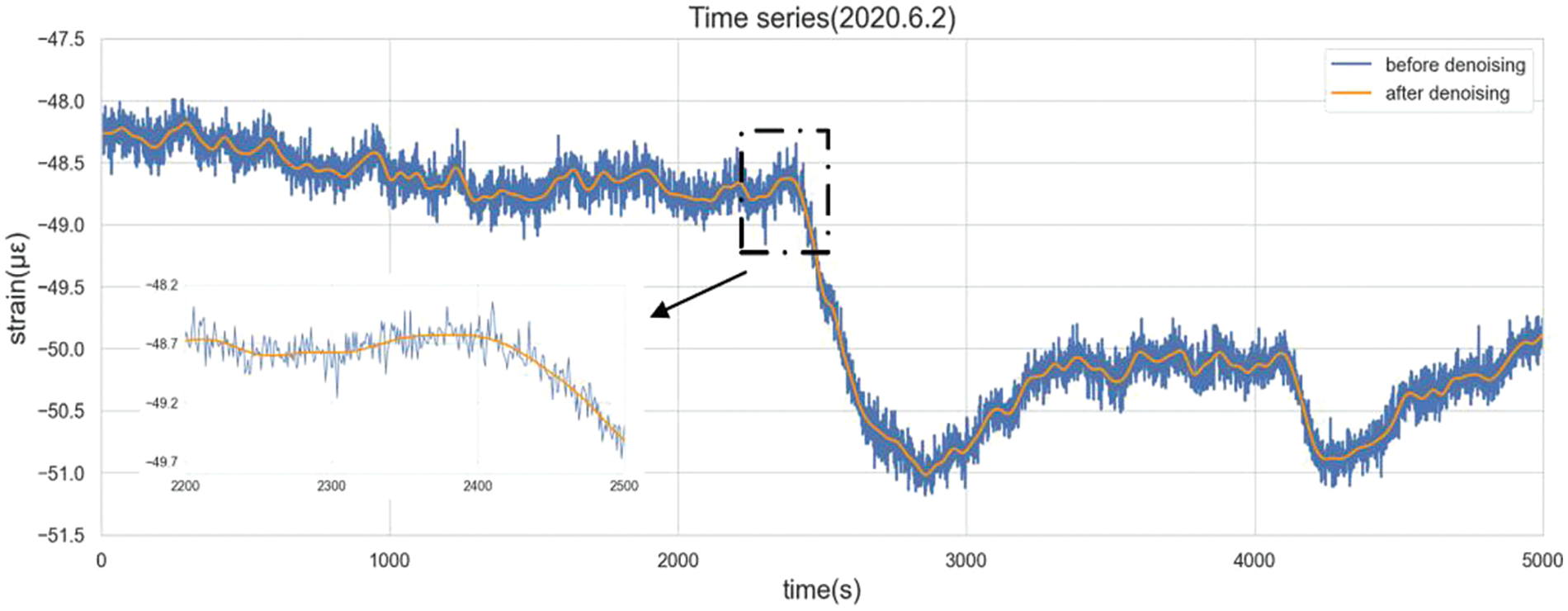
Figure 6: Time series before and after denoising (according to Chen et al. [39])

This study adopts wavelet threshold denoising method to eliminate noise. Specifically, the original data undergoes decomposition into five layers using Symlet 12 as the mother wavelet, for which the details were as obtained from the literature [42].

3.3 Establishment of the ARIMA-Based Model

3.3.1 Data Preprocessing

For the ARIMA model, the time series used should exhibit both stationarity and absence of white noise after differencing. Given ARIMA’s appropriateness for short-term predictions and the usual availability of historical modeling data containing fewer than 10 observations (resulting in p and q values predominantly below 10), this study adopts a dataset of 100 observations (equivalent to a 100-second time window) to develop the model. As an illustrative example, a time series of denoised concrete strain data from the HZMB immersed tunnel is employed, as depicted in Fig. 7.

Figure 7: Time series of concrete strain data from the HZMB immersed tunnel on June 02, 2020 (sourced from Chen et al. [39])

Table 2 provides insight into the initial series and the differenced series’ timing graphs, along with the Autocorrelation Function (ACF) plots and Partial Autocorrelation Function (PACF) plots. The timing graph of the second differentiated series exhibits no discernible trend, amplitude variation, or frequency change. Based on this observation, a preliminary judgment was made that the sequence aligns with the criteria for stationarity.

The Augmented Dickey-Fuller (ADF) test was employed to statistically evaluate the stationary of data, and the results are presented in Table 3. Consequently, the value of d, representing the order of differencing, was determined as two.

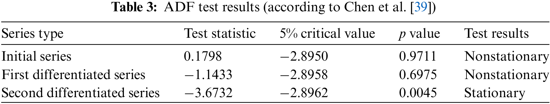
Finally, the Ljung-Box test was utilized to discern the presence of white noise in the second differentiated series. The p value of the second differenced series was 2.29 × 10−22, signifying that the series did not exhibit white noise characteristics, warranting further analysis.

3.3.2 Model Identification

The process of model identification is to set the number of Autoregressive (AR) and Moving Average (MA) terms by an optimization calculation. This study employs the Akaike Information Criterion (AIC) and Bayesian Information Criterion (BIC) to automatically select p and q, utilizing a 100-second time window of SHM data. As evident from the results presented in Table 4, optimal values of (p,d,q) were set as (5,2,0).

Thus, the ARIMA-based model's formulation is as follows:

∇2Xt=φ1∇2Xt−1+φ2∇2Xt−2+…+φ5∇2Xt−5+εt(7)

3.3.3 Static ARIMA Model

The parameter estimation method selected here is Maximum Likelihood Estimation (MLE) method. Fig. 8 shows the results of parameter estimation, and the meanings of corresponding parameters were as given in the literature [40].

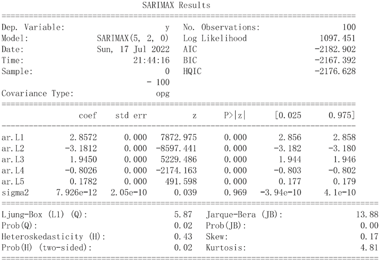
Figure 8: Parameters estimation of static ARIMA (sourced from Chen et al. [39])

The model's significance was assessed and illustrated in Fig. 9 (for which the explanatory note is the same as given in the literature [39]). Collectively, these results affirmed the model's significance.

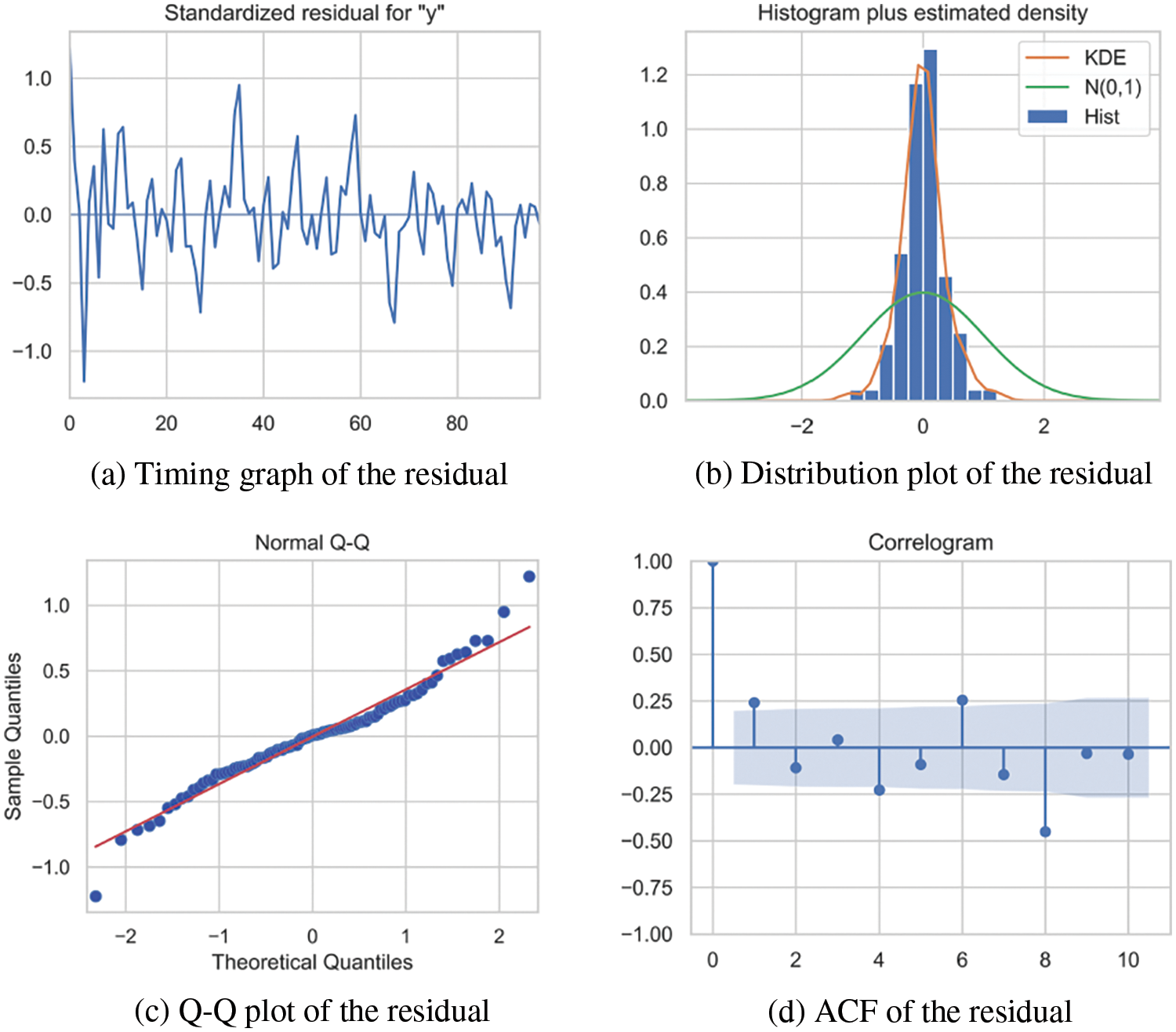
Figure 9: Assessment plots of the model's significance (sourced from Chen et al. [39])

Fig. 10 illustrates the point prediction and prediction intervals derived from the model over a ten-step forecast at different time points. Notably, ARIMA’s predictive accuracy was strong within the initial five-time steps; however, accuracy gradually diminished as the forecast horizon extended.

Figure 10: Static ARIMA prediction at different time points (redrawn according to Chen et al. [39])

3.3.4 Dynamic ARIMA Model

In this study, a model error monitoring approach is adopted to determine when model updates are required. The system automatically updates parameters based on the latest 100 s of observations. Test results revealed that selecting an update threshold of 5 × 10−8 prompted the model to update 29 times in a day. The error sequence exhibited steady fluctuations throughout the day, as depicted in Fig. 11. The sustained error levels over time confirmed that the model error monitoring approach effectively ensures the accuracy of dynamic ARIMA model.

Figure 11: Dynamic ARIMA error sequence (according to Chen et al. [39])

3.4 Establishment of the LSTM-Based Model

3.4.1 Data Preprocessing

When utilizing filtered data to construct an LSTM model, a noticeable lag in predicted values occurs when the data experiences rapid rises or falls (refer to Fig. 12). Examining the finer details in Fig. 13, it becomes evident that the predicted value at time t+1 closely resembles the input value at time t or some period prior.

Figure 12: Model validation (constructed using initial series)

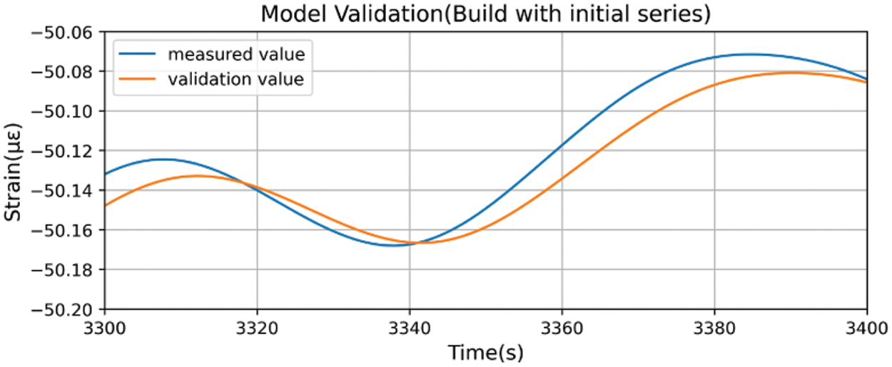
Figure 13: Model validation (constructed using initial series) (Zoomed in)

During prediction for time t+1, the model might learn to simply adopt the value from the preceding time as the forecasted value, as this could minimize errors across the board, aligning with optimization objectives. However, this approach does not harness any meaningful features, essentially yielding a sequence replication. The pronounced lag in prediction is evidently invalid.

There are two ways to solve this hysteresis. One is to apply a nonlinear function, such as the square, square root, and logarithm, to the sequence. The other is to differentiate the sequence until it is stationary. The first method requires nonlinear processing, thus changing the original sequence more radically. Moreover, the first method relies on the fact that the constructed nonlinear processing function is not recognized by the regressor of LSTM, but based on the experience of previous studies, this method has a high probability of failure and usually involves trying many different nonlinear processing functions [43]. The second method, on the other hand, is somewhat more generalizable. To build a model more robust and closer to the real situation, the second method is adopted in this paper.

Due to the iterative optimization of network parameters based on training set errors, model errors within the training set typically appear lower than actual errors. Consequently, sample data is divided into a training set and a test set. Striking a balance between training duration and model accuracy, this paper assigned 5/6 of the data instances to the training set and reserved the remaining 1/6 for the testing set. With a window width of 3600 s, the initial 3000 s were allocated for the training set, while the final 600 s formed the test set. The partitioning outcomes are depicted in Fig. 14.

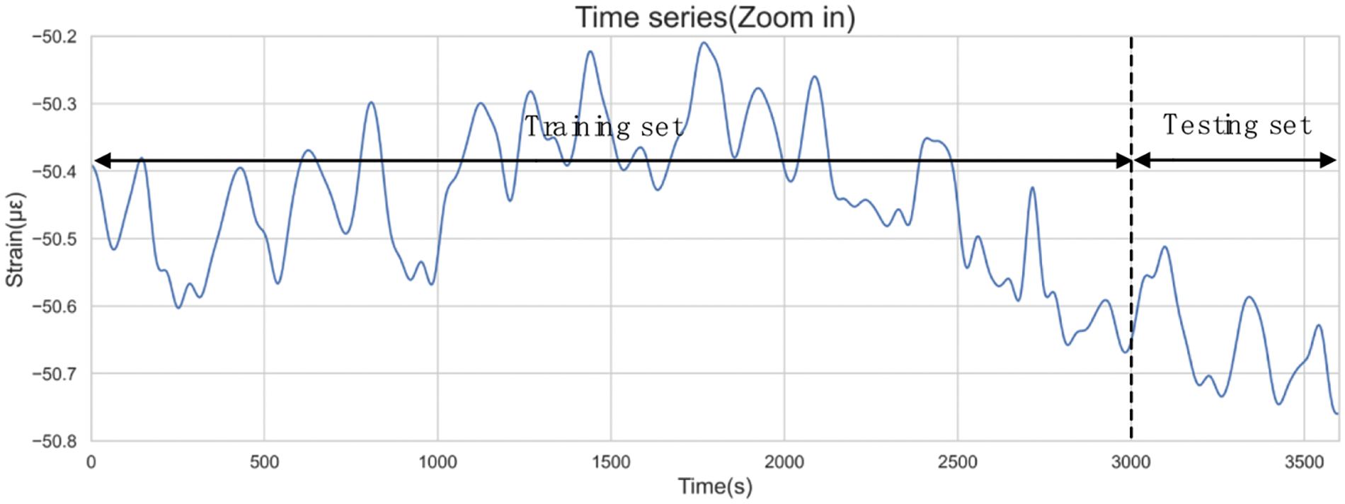
Figure 14: Data split results

Training samples should be transferred to a standard form so that they can be learned by neural networks. According to Section 2.3, the input of the training sample Xt should be the sequence value within the time window with a certain length, and the training label Y should be the sequence value at the next second of the time window. At each time step, the time window moves forward to obtain a new input sequence for a training label. As the fixed-size sliding window passes over the sequence from left to right, a series of input sequences and training labels are formed. As a result, a series of Xt and Y are obtained, with a one-to-one correspondence along the timeline. This process is shown in Fig. 15.

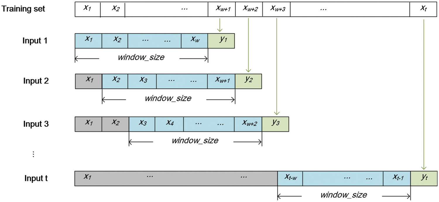
Figure 15: Standardized format of training samples

3.4.2 Hyperparameter Tuning

The main hyperparameters of LSTM include the number of hidden layers, the number of units at each layer, time window length, batch size, and number of epochs. To reduce the time of tuning, the model structure was set as a two-layer LSTM network with a batch size of 50 and an epoch number of 50. A discrete grid was set for the remaining hyperparameters, and a grid search was conducted to find the satisfying combination of hyperparameter values. Specifically, each grid value combination was used to train the network. The optimal performance combination was selected by evaluating the Mean Squared Error (MSE) of the model on the test set.

Because the weights are randomly initialized, the LSTM is unstable, meaning that the model's outcome varies even when the training data remains unchanged. To obtain a reliable model performance, each hyperparameter combination undergoes training ten times repeatedly, and the performance metrics are calculated by the overall mean of the absolute error on the test set. Table 5 lists the specific values and the optimal results of the hyperparameter tuning. It should be noted that this procedure of hyperparameter tuning was necessary because these hyperparameters have a large impact on the accuracy of the model output.

The output dimension of the second LSTM layer is the same as the dimension of the units in this layer, while the output of the model needs to be consistent with the dimension of label Y. Therefore, after two LSTM layers, a fully connected dense layer was added to carry out dimensional transformation. In summary, the network structure of the LSTM model in this paper is shown in Fig. 16.

Figure 16: LSTM network structure

3.4.3 Static LSTM Model

After standardizing training data and selecting hyperparameters, the parameters of the model can be trained iteratively. The adaptive moment estimation algorithm serves as the optimizer, dynamically setting the learning rate by assessing gradients’ first and second moments. The Mean Squared Error (MSE) was selected as the loss function. It is one of the most commonly used loss functions in machine learning and gives a high penalty for outliers in sequences.

To avoid the influence of randomness on the model, the network was repeatedly trained 50 times, and the distribution of MSE on the test set was recorded. The distribution was skewed to the right, as shown in Fig. 17. This indicated that most LSTM models exhibit small errors, but there were also a few cases where the errors are significantly greater than the average. Striking a balance between training duration and model quality, the model maximum allowable error was set as MSE < 2 × 10−8. If the error exceeds this threshold, random weights are reset, and the model undergoes retraining until it satisfies the error criteria.

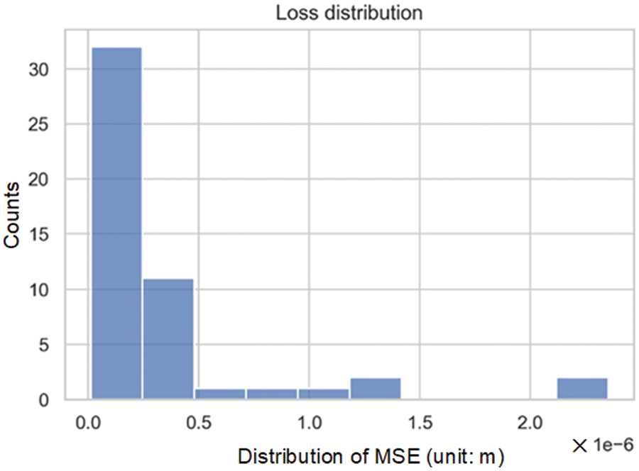
Figure 17: Loss distribution within the test set

Fig. 18 shows the change curves of MSE on the training set and the validation set during the 50 iterations. After 30 iterations, the test set error stabilized, approaching the training set error. This indicated that the model did not experience underfitting or overfitting problems and that the number of epochs could be set as 30.

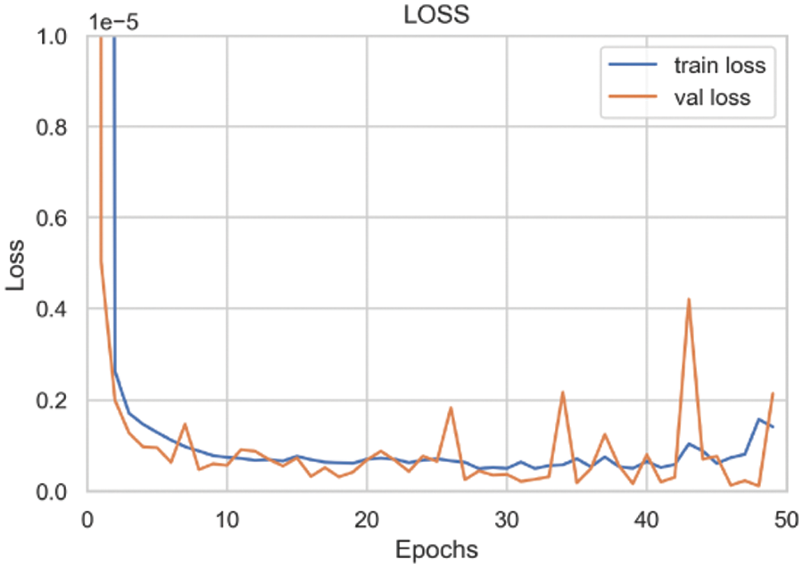
Figure 18: MSE loss during the training process

Fig. 19 shows that the model learned the dependencies of the sequence well and achieved good model performance. The prediction coincided with the observation in general and only made a slight error when the observation changed rapidly. The model was ready for the needs of subsequent anomaly detection.

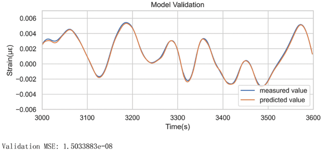
Figure 19: Model prediction values and measured values within the validation set

Fig. 20 was obtained by inversing the differencing operations. A comparison between model prediction details on the test set built with the original sequence (Fig. 13) and the differenced sequence (Fig. 21) underscored the efficacy of differencing preprocessing in mitigating the hysteresis phenomenon.

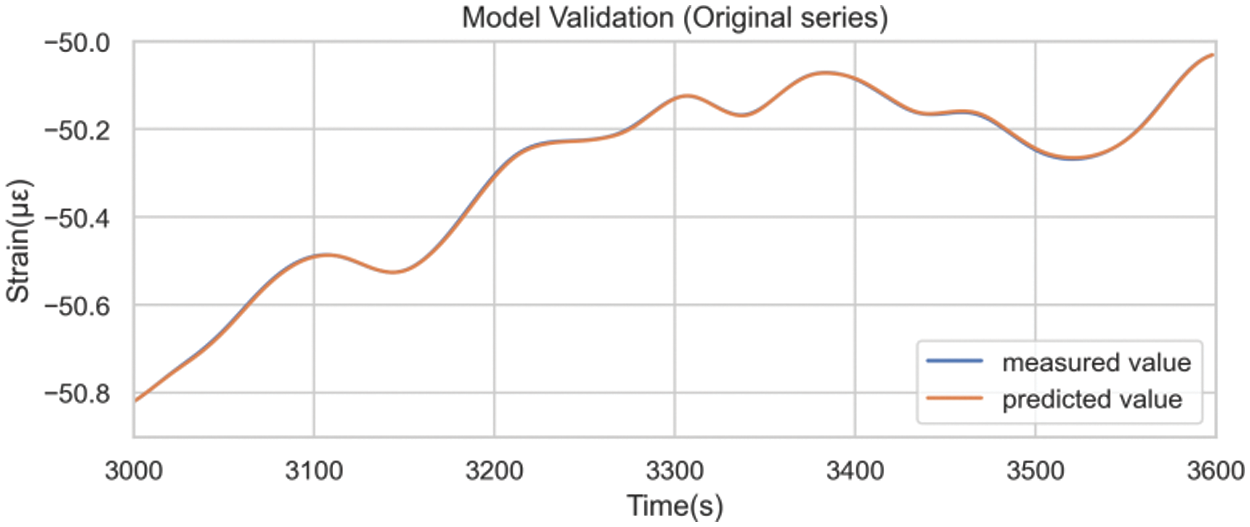
Figure 20: Model prediction results after inverting the difference

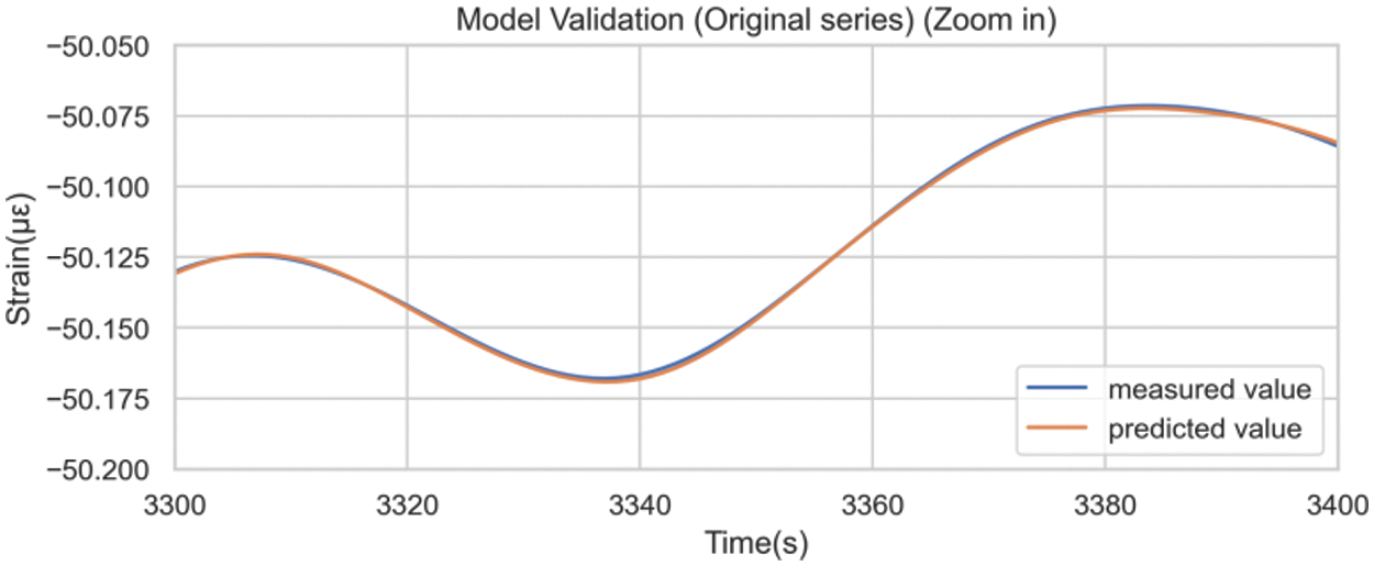
Figure 21: Model prediction results after inversing the difference (Zoomed in)

3.4.4 Dynamic LSTM Model

Parallel to the ARIMA model, this section delves into the dynamic modeling approach for LSTM. Based on test results, the LSTM model maintained robust prediction performance for at least an hour after fitting. Rebuilding the LSTM is time-intensive due to the model’s parameter complexity and the iterative training required to mitigate randomness effects. Thus, the model’s update interval was set to one hour. Precisely, adhering to the identical LSTM network framework and hyperparameters, the LSTM model is retrained every hour using data from the preceding hour. The training set to test set ratio remains at 5:1. Through this approach, the model updates with data from the previous hour, inheriting the prior hour's initial parameters to expedite model training. Dynamic modeling maintains the maximum allowable error standard established in the static model, indicating the training loop halts only when the model's MSE falls below 2 × 10−8.

Similar to the ARIMA model, the dynamic LSTM modeling approach is discussed in this section. Based on test results, the LSTM model maintained robust prediction performance for at least 1 h after fitting. Rebuilding the LSTM is time-intensive due to the model’s parameter complexity and the iterative training required to mitigate randomness effects. Thus, the model’s update interval was set to 1 h. Specifically, by keeping the LSTM network framework structure and hyperparameters unchanged, the LSTM model would be retrained every hour based on the data of the previous hour, with a training set and test set in the ratio of 5:1. Through this approach, the model was updated with data from the previous hour, inheriting the prior hour's initial parameters to expedite model training. Dynamic modeling was set to continue to use the maximum allowable error set in the static model, which means that the training loop would stop only if the MSE of the model fell below 2 × 10−8.

Due to the large amount and the similarities among SHM data, other SHM data (such as ground motion and joint deformation) were not analyzed for validation in this study. The temperature and humidity, which are categorized as environmental loads, are strongly influenced by natural conditions and need to be analyzed separately. Therefore, a two-day concrete strain data sample was introduced for model training of the LSTM network. Fig. 22 shows the dynamic LSTM model error over time, revealing a declining error initially, followed by stabilization within a narrow range. This demonstrated that the neural network could learn the characteristics of data during a long-term process and continuously optimize itself.

Figure 22: LSTM model error (built with the concrete strain data on June 1st and June 2nd)

4  Comparative Analysis of Anomaly Detection Results

4.1 Anomaly Detection Results Using the ARIMA-Based Model

The prediction error for a 1 h duration, which represents the discrepancy between the ARIMA model's one-step prediction and the actual observation, was calculated. As depicted in Fig. 23, the prediction error basically followed a normal distribution, which indicated that dynamic thresholds could be set based on the statistical feature of the previous hour.

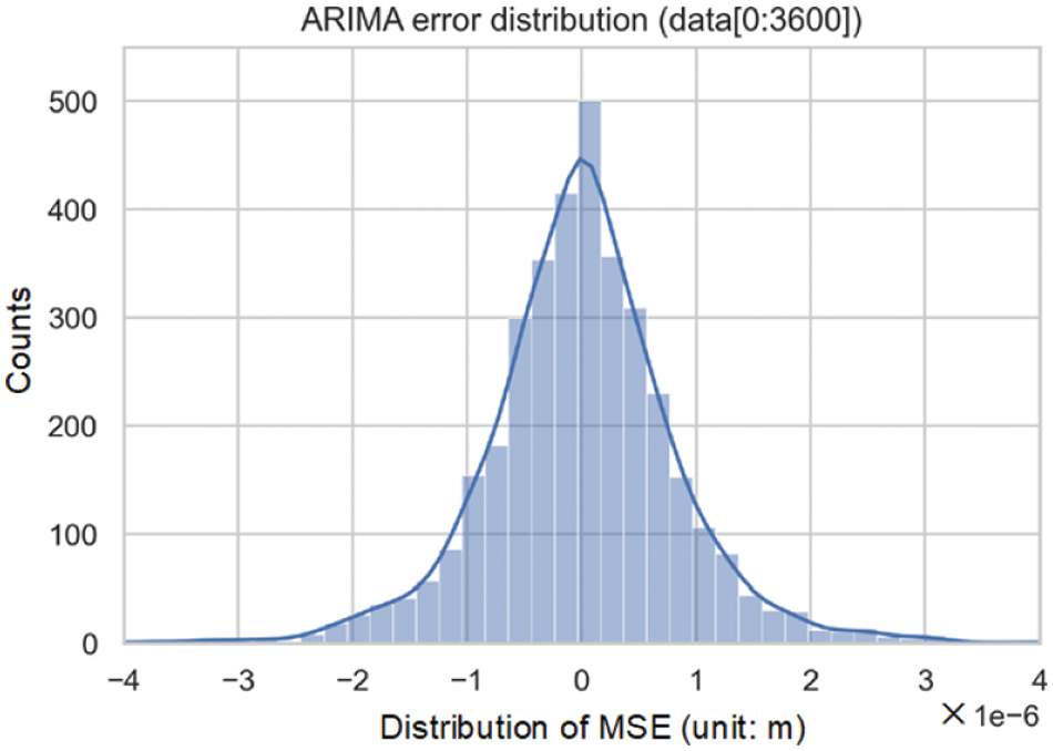
Figure 23: Distribution of one-hour prediction errors from the dynamic ARIMA model

Given that standard deviation gauges data variance, the previous hour’s data standard deviation was employed to gauge the permissible range of error fluctuations. By adjusting the coefficient of standard deviation, the confidence interval of different severities was set to realize the hierarchical warning. Utilizing thresholds set at 5.5, 6.5, and 7.5 standard deviations, outliers could be identified, as illustrated in Fig. 24.

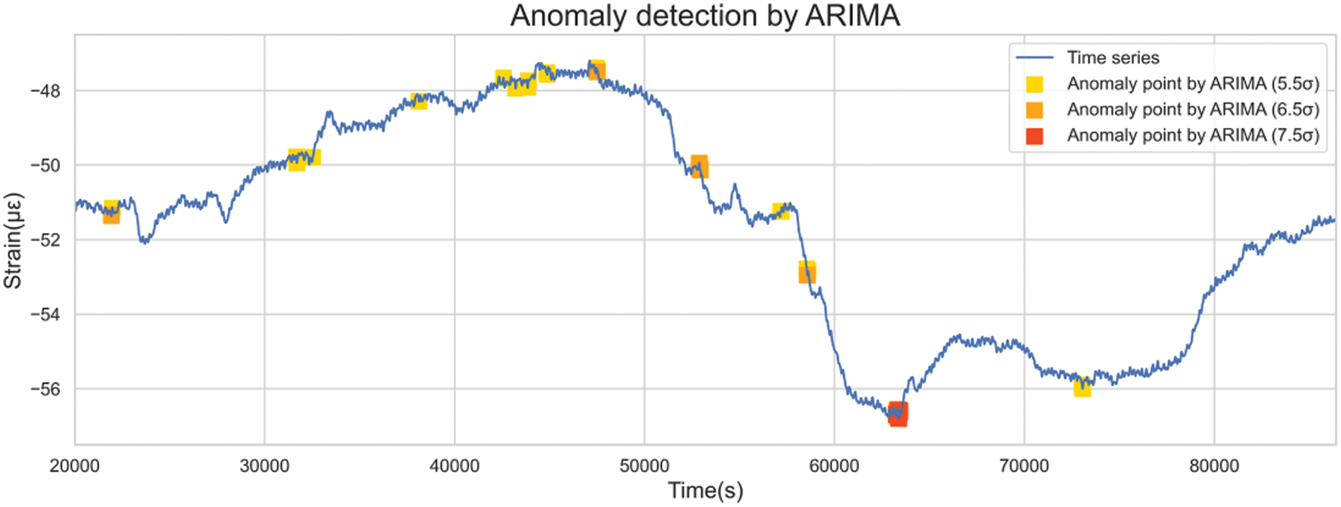
Figure 24: Detection of anomalies of different severity levels by the ARIMA-based model

4.2 Anomaly Detection Results Using the LSTM-Based Model

The anomaly detection mechanism employed by the dynamic LSTM model closely resembles that of ARIMA. Fig. 25 shows that the distribution of the prediction error resembled a bell-shaped curve, underscoring the potential to derive dynamic thresholds that correspond to diverse confidence intervals via varying standard deviation multiples.

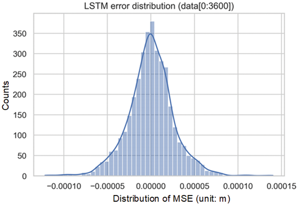
Figure 25: Distribution of one-hour prediction errors from the dynamic LSTM model

Thresholds of 5.5, 7, and 8 standard deviations were employed to identify outliers, as highlighted in Fig. 26.

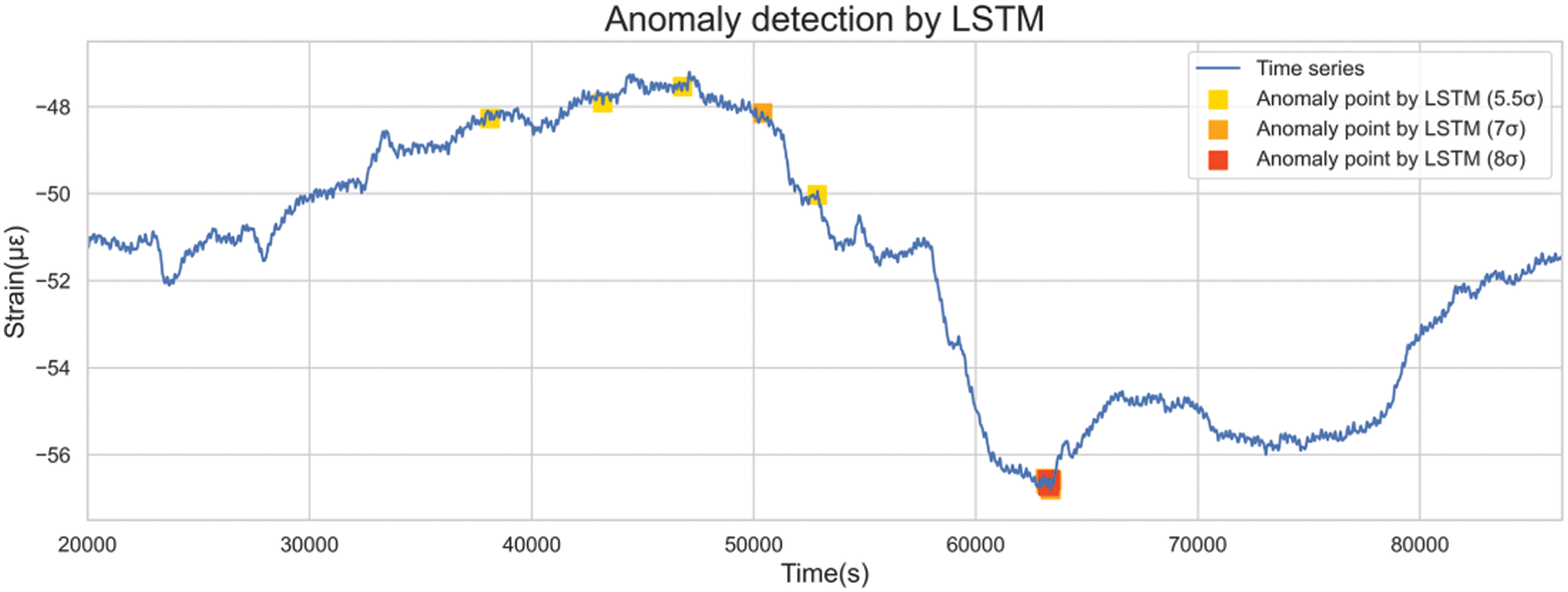
Figure 26: Detection of anomalies of different severity levels by the LSTM-based model

4.3 Comparative Analysis of the Two Models

4.3.1 Modeling Efficiency and Computational Performance

Considering the sequence requirements, the ARIMA model necessitates a stationary nonwhite noise sequence for effective modeling. In contrast, LSTM exhibits wider applicability due to its non-restrictive nature. LSTM merely demands the partitioning of original data into training samples and labels, thereby enabling broader adaptability compared to the ARIMA model.

Sample size plays a pivotal role in modeling. ARIMA requires a substantial sample size for statistical inference, with studies indicating a minimum requirement of at least 50 historical data points for acceptable results [44]. As ARIMA predominantly focuses on analyzing near-future temporal data changes with small order parameters, further enlarging the sample size does not proportionally enhance model quality. In contrast, LSTM, being a complex neural network, thrives on larger data volumes for proper training. The larger the sample size is, the more materials the LSTM model will learn, and its accuracy will be improved. Therefore, LSTM requires a larger sample size than ARIMA and benefits from more samples.

In terms of modeling speed, LSTM involves more parameters and intricate structures than ARIMA, leading to longer iterative calculations for parameter adjustments. Experimental evidence indicates that static ARIMA modeling can be completed in a mere 0.55 s, whereas static LSTM modeling takes approximately 131.7 s. Hence, ARIMA significantly surpasses LSTM in modeling speed. Both models ran on the same laptop with the following hardware information: an Intel Core i7-10750H processor with 16 GB of RAM, 1TB SSD hard disk, graphics card NVIDIA GeForce RTX 2060 Max-Q.

Regarding model stability, ARIMA operates deterministically; given data and hyperparameters, estimated model parameters are deterministic. In contrast, LSTM's modeling process is influenced by random factors like initial weight settings and batch selection, contributing to variable model outcomes across runs. To ensure accuracy, repeated modeling and setting of maximum acceptable errors are integrated into LSTM training. Consequently, ARIMA results tend to exhibit greater model stability than LSTM results.

4.3.2 Thresholds and Graded Anomalies

Fig. 27 illustrates the impact of different standard deviation coefficients on detected anomaly proportions. As the coefficient increased, the threshold became stricter, resulting in fewer detected anomalies.

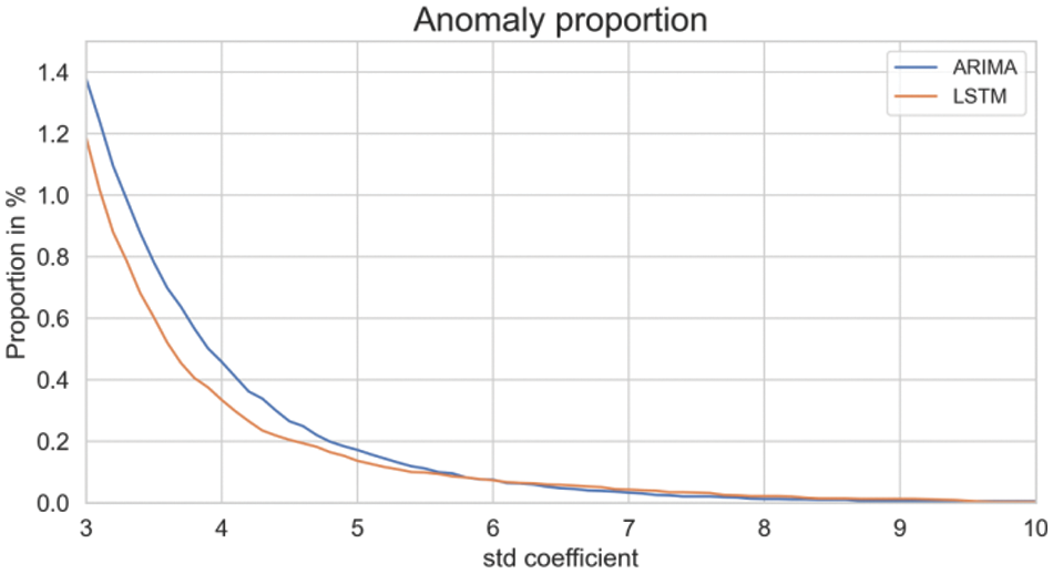
Figure 27: Detected anomaly proportions varying with different standard deviation coefficients

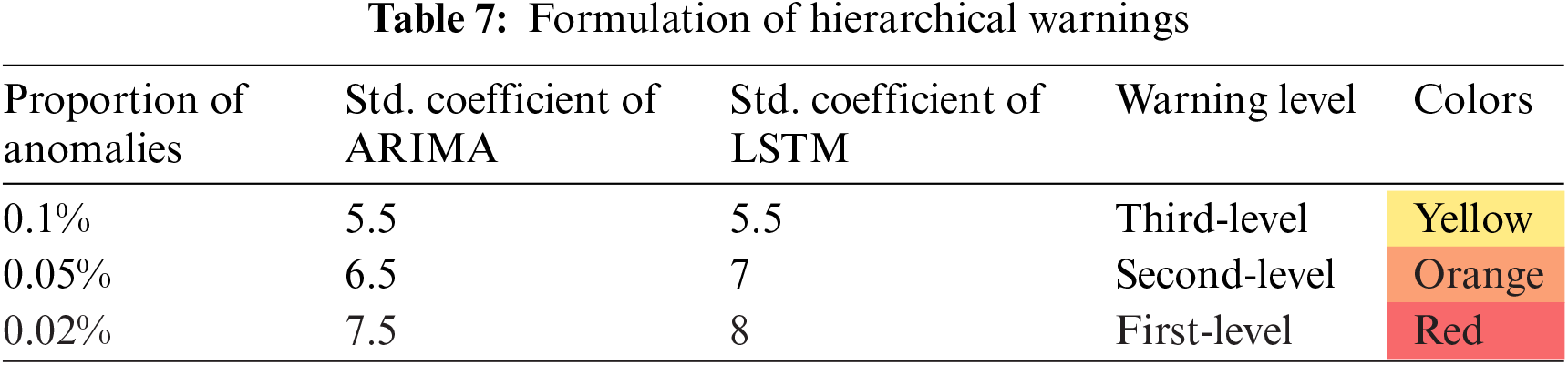
For a fair comparison, it is necessary to establish the anomaly detection criteria. Table 6 outlines the anomaly count and proportion with specific coefficients’ multiple standard deviation serving as thresholds.

Hierarchical warnings are formulated based on anomaly proportions, with corresponding thresholds established, as indicated in Table 7. With hierarchical warnings, tunnel operators can take measures for anomalies of varying severity.

4.3.3 Timing of Warnings and Characteristics of Detected Anomalies

This section delves into the distribution and specifics of anomalies identified by both models across first to third-level thresholds. To provide a clearer perspective, anomalies from both methods are plotted on the same graph.

1) First-Level Warning

First-level warnings have the largest standard deviation coefficient, the strictest identification standard, and the fewest outliers identified. These require immediate attention and emergency measures from operational personnel. As shown in Fig. 28, the distributions of the first-level anomalies identified by the two methods were consistent, both at the inflection point, where the sequence changes from the original downward trend to an upward trend.

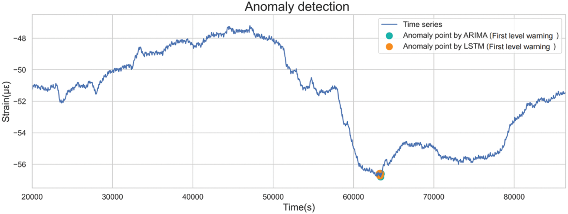
Figure 28: Distributions of the first-level anomalies

Fig. 29 demonstrates that LSTM detected first-level anomalies earlier than ARIMA. The discrepancy in anomaly detection timing indicated differing underlying logic. The anomalies identified by ARIMA were detected after the change in data trends occurred, where the sequence started to change rapidly. LSTM recognized the outliers earlier when the frequency of the sequence was significantly larger compared with the previous sequence. Such collective anomaly in the data often indicates a change in trend, enabling LSTM to offer early warnings.

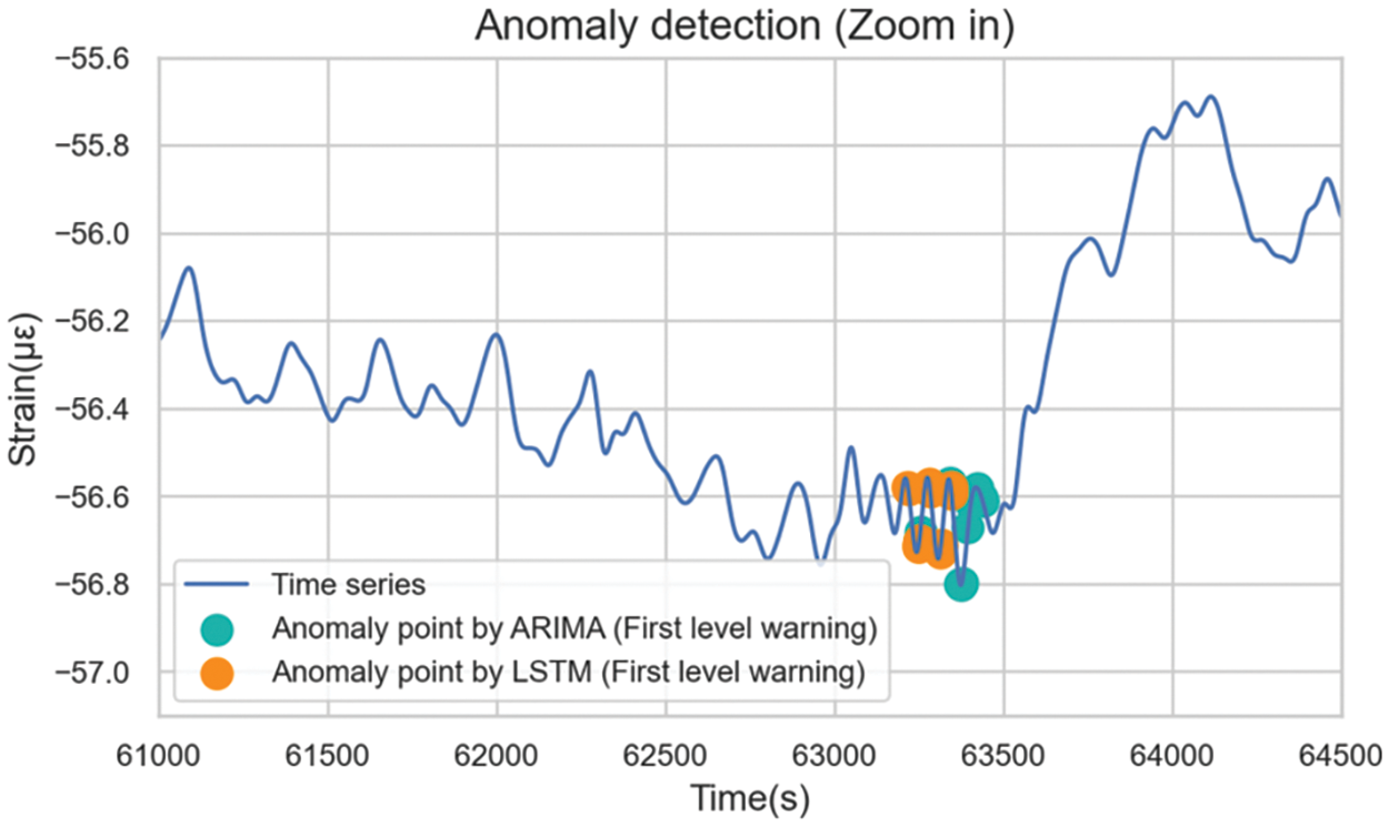
Figure 29: Details of the first-level anomalies

2) Second-Level Warning

Second-level warnings are issued when anomalies are detected according to moderate standards. Fig. 30 shows the distribution of second-level anomalies. Although anomalies detected by both methods were not entirely congruent, both models issued warnings near daily high and low points. Frequent warnings were also observed between 5,000 and 6,000 s, corresponding to steep data declines.

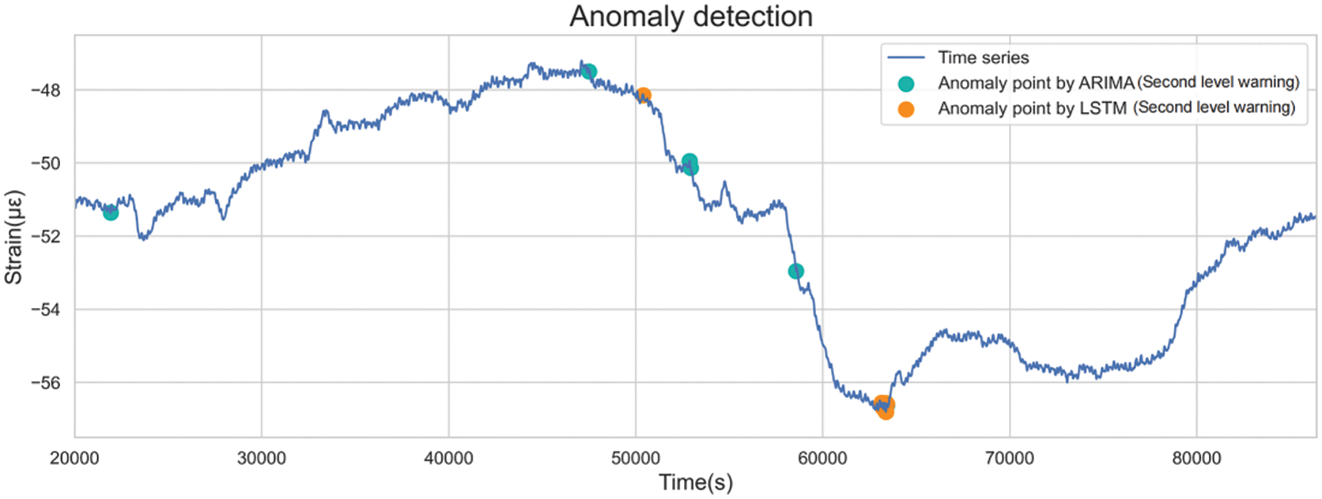
Figure 30: Distributions of the second-level anomalies

3) Third-Level Warning

With more liberal anomaly detection criteria, third-level warnings encompass numerous anomalies with relatively mild severity (Fig. 31). A comprehensive comparison and analysis of the characteristics of the two methods was facilitated due to the great anomaly count.

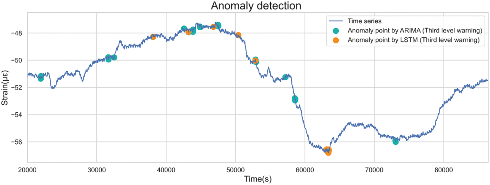
Figure 31: Distributions of the third-level anomalies

LSTM identified fewer anomalies in specific locations compared to ARIMA, attributed to divergent prediction data windows. For instance, ARIMA predicted using historical data from the last 5 s, while LSTM employed 100 s. Thus, if the value drops rapidly for 10 s at the same rate, ARIMA will not alarm for the last 5 s; LSTM, on the other hand, alerts all data within 10 s, being more sensitive to extended data changes.

Moreover, both models exhibited increased warnings between 40,000 and 50,000 s, corresponding to the day’s data peak. It was supposed that before the data trend changed, other hidden features, such as amplitude and frequency, fluctuated in advance. The LSTM model could detect such changes and provide an early warning.

Fig. 32 illustrates anomalies exclusively identified by either model, revealing distinct strengths. ARIMA swiftly detected drastic recent value changes, indicating potential structural issues. On the other hand, LSTM recognized changes earlier, thanks to its capacity to discern patterns from extended historical data. Figs. 32a and 32b are the anomalies recognized only by ARIMA. ARIMA used fewer historical observations for each prediction, which could efficiently detect the anomalies with drastic changes in recent values. Dramatic changes in a short period may cause structural damage, which requires timely investigation and removal of potential safety hazards. However, these anomalies do not necessarily represent structural damage, but may only represent severe vibration in a very short period of time. Therefore, continuous attention should be paid to subsequent sequence changes before making operational and maintenance decisions. Figs. 32c and 32d are the anomalies identified only by LSTM. If the signal behind the outlier is covered, it is difficult to distinguish the abnormal situation by the naked eye. However, the trend of the sequence did change soon after the warning. This showed that LSTM could learn the potential features of the sequence from a longer historical data window and predict the trend change in advance. As shown in Figs. 32e and 32f, ARIMA usually sent out an early warning just after the occurrence of anomalies, while LSTM could always identify data trend changes much earlier.

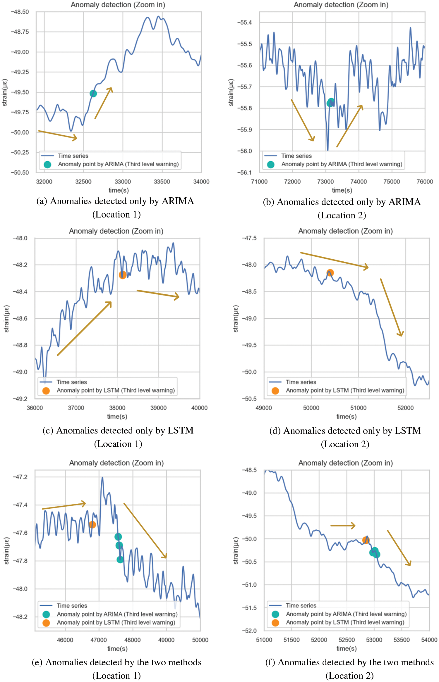
Figure 32: Details of the third-level anomalies

4.3.4 Comparison Summary

Based on the preceding analysis, the two models exhibited distinct characteristics, summarized in Table 8.

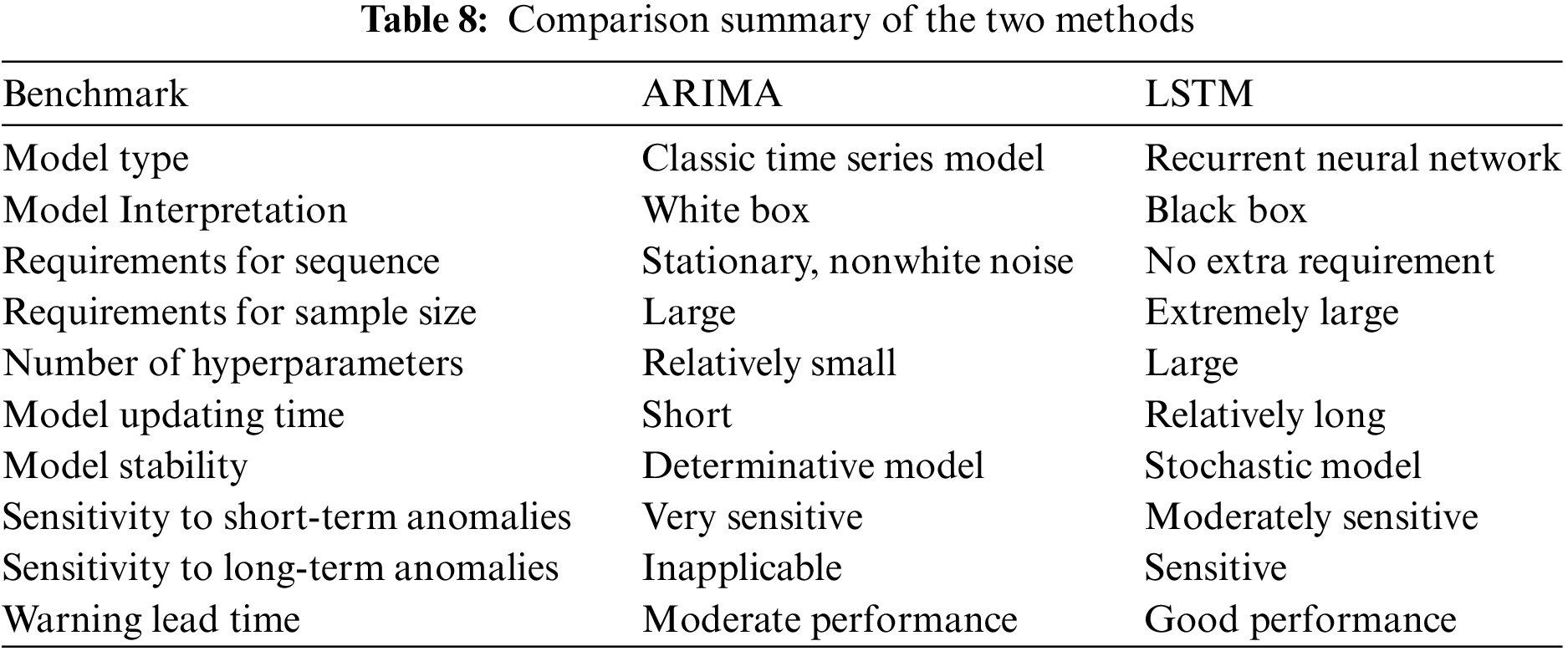
In conclusion, LSTM has fewer sequence constraints during modeling, but necessitates a larger sample size and presents a more intricate, less interpretable model. While ARIMA is adept at detecting short-term sequence fluctuations, its ability to detect medium- to long-term anomalies is limited. Moreover, ARIMA tends to issue warnings post-anomaly occurrence, leading to unsatisfied timing of early warning. On the contrary, LSTM demonstrates greater proficiency in predicting long-term sequence trends and delivering better performance of early warnings. One point to mention is that there is a difference in data applicability between ARIMA and LSTM, with ARIMA being stricter on the data and requiring a series of statistical testing and validation, as demonstrated in Section 3.3.3. This may lead to limitations in the application of ARIMA.

For a tunnel SHM system, a large data set is ready for deep learning, so the learning potential of the LSTM model can be fully utilized. Generally, LSTM yields more accurate anomaly detection outcomes than ARIMA. However, ARIMA’s advantage in monitoring short-term sequences should not be disregarded. Therefore, combining these methods effectively—using LSTM as the primary method for long-term trend monitoring and early warning, while employing ARIMA as a supplementary tool with stringent threshold criteria for prompt short-term anomaly identification—seems promising for future monitoring system designs.

5  Conclusion

This study presented a hierarchical model-based approach for anomaly detection and evaluated it by a comparative analysis using SHM data from the HZMB immersed tunnel. The conclusions are as follows:

1.    The concrete strain data of immersed tunnel elements were used in this paper, both ARIMA and LSTM could realize the dynamic model-based approach for anomaly detection. The model structure of ARIMA was ARIMA (5, 2, 0), and its modeling time was shorter, which took only 0.55 s; LSTM consisted of 1961 parameters, which needed to spend 131.7 s for modeling. However, ARIMA was slightly weaker than LSTM in prediction accuracy, thus using different criteria for updating the rolling dynamic model (5 × 10−8 for ARIMA and 2 × 10−8 for LSTM). Therefore, in terms of modeling features, ARIMA has better real-time performance and LSTM has better prediction accuracy.

2.    Dynamic model-based approach uses specific coefficients multiple standard deviation as an outlier screening criterion. ARIMA-based and LSTM-based model use very similar coefficients. For the first-level warning, which is the strictest, the coefficients of the two were roughly in the range of 7.5 to 8. For the second-level warning, the coefficients of the two were roughly in the range of 6.5 to 7. For the third-level warning, the coefficients of the two were both 5.5. This suggests that there is actually little difference between the two in terms of their ability to identify outlier data.

3.    In terms of data requirements, the ARIMA-based model requires stationary, nonwhite noise sequences, while the LSTM-based model has no additional sequence requirements. The comparative analysis of the two models indicated that ARIMA was highly sensitive to short-term anomalies, whereas LSTM was sensitive to long-term anomalies, leading to the phenomenon that LSTM performed better in early warnings. Therefore, it suggests combining LSTM for long-term trend monitoring and early warning with ARIMA as a supplementary tool for swift short-term anomaly identification.

Acknowledgement: We acknowledge the support given by the Hong Kong-Zhuhai-Macao Bridge Authority.

Funding Statement: This work was supported by the Research and Development Center of Transport Industry of New Generation of Artificial Intelligence Technology (Grant No. 202202H), the National Key R&D Program of China (Grant No. 2019YFB1600702), and the National Natural Science Foundation of China (Grant Nos. 51978600 & 51808336).

Author Contributions: The authors confirm their contributions to the paper as follows: study conception and design: Q. Ai, Q. Lang; data collection: X. Jiang, Q. Jing; analysis and interpretation of results: Q. Ai, H. Tian, H. Wang, X. Huang, X. Jiang, Q. Jing; draft manuscript preparation: Q. Ai, Q. Lang. All authors reviewed the results and approved the final version of the manuscript.

Availability of Data and Materials: Data is available on request to the authors.

Conflicts of Interest: The authors declare that they have no conflicts of interest to report regarding the present study.

References

1. Inaudi, D. (2009). Structural health monitoring of bridges: General issues and applications. In: Structural health monitoring of civil infrastructure systems, pp. 339–370. UK: Woodhead Publishing. [Google Scholar]

2. Zhang, X., Broere, W. (2023). Design of a distributed optical fiber sensor system for measuring immersed tunnel joint deformations. Tunnelling and Underground Space Technology, 131, 104770. [Google Scholar]

3. Zhang, X., Broere, W. (2023). Monitoring seasonal deformation behavior of an immersed tunnel with distributed optical fiber sensors. Measurement, 219, 113268. [Google Scholar]

4. Zhang, X., Broere, W. (2023). Monitoring of tidal variation and temperature change-induced movements of an immersed tunnel using distributed optical fiber sensors (DOFSs). Structural Control and Health Monitoring, 2023, 2419495. [Google Scholar]

5. Zhang, K., Qi, T., Li, D., Xue, X., Zhu, Z. (2021). Load testing and health monitoring of monolithic bridges with innovative reinforcement. International Journal of Structural Integrity, 12(6), 904–921. [Google Scholar]

6. Moyo, P., Brownjohn, J. M. W. (2002). Detection of anomalous structural behaviour using wavelet analysis. Mechanical Systems and Signal Processing, 16(2–3), 429–445. [Google Scholar]

7. Ai, Q., Yuan, Y., Shen, S. L., Wang, H., Huang, X. (2020). Investigation on inspection scheduling for the maintenance of tunnel with different degradation modes. Tunnelling and Underground Space Technology, 106, 103589. [Google Scholar]

8. Ai, Q., Yuan, Y. (2018). State-oriented maintenance strategy for deteriorating segmental lining of tunnel. Journal of Civil Engineering and Management, 24(6), 469–480. [Google Scholar]

9. Ai, Q., Yuan, Y., Jiang, X., Wang, H., Han, C. et al. (2022). Pathological diagnosis of the seepage of a mountain tunnel. Tunnelling and Underground Space Technology, 128, 104657. [Google Scholar]

10. Sun, F., Li, C. (2022). A comprehensive evaluation method and application of shield tunnel structure health based on variable weight theory. International Journal of Structural Integrity, 13(3), 394–410. [Google Scholar]

11. Farrar, C. R., Park, G., Farinholt, K. (2009). Structural Health monitoring with autoregressive support vector machines. Journal of Vibration and Acoustics, 131, 021004–1. [Google Scholar]

12. Maes, K., Salens, W., Feremans, G., Segher, K., François, S. (2022). Anomaly detection in long-term tunnel deformation monitoring. Engineering Structures, 250, 113383. [Google Scholar]

13. Nguyen, L. H., Goulet, J. A. (2018). Anomaly detection with the switching kalman filter for structural health monitoring. Structural Control and Health Monitoring, 25(4), e2136. [Google Scholar]

14. Nguyen, L. H., Goulet, J. A. (2019). Real-time anomaly detection with Bayesian dynamic linear models. Structural Control and Health Monitoring, 26(9), e2404. [Google Scholar]

15. Zhang, Y. M., Wang, H., Wan, H. P., Mao, J. X., Xu, Y. C. (2021). Anomaly detection of structural health monitoring data using the maximum likelihood estimation-based Bayesian dynamic linear model. Structural Health Monitoring, 20(6), 2936–2952. [Google Scholar]

16. Tang, Z., Chen, Z., Bao, Y., Li, H. (2019). Convolutional neural network-based data anomaly detection method using multiple information for structural health monitoring. Structural Control and Health Monitoring, 26(1), e2296. [Google Scholar]

17. Bao, Y., Tang, Z., Li, H., Zhang, Y. (2019). Computer vision and deep learning-based data anomaly detection method for structural health monitoring. Structural Health Monitoring, 18(2), 401–421. [Google Scholar]

18. Du, Y., Li, L. F., Hou, R. R., Wang, X. Y., Tian, W. et al. (2022). Convolutional neural network-based data anomaly detection considering class imbalance with limited data. Smart Structures and Systems, 29(1), 63–75. [Google Scholar]

19. Entezami, A., Sarmadi, H., Behkamal, B. (2023). Long-term health monitoring of concrete and steel bridges under large and missing data by unsupervised meta learning. Engineering Structures, 279, 115616. [Google Scholar]

20. Wang, H., Li, L., Li, J., Sun, D. A. (2022). Drained expansion responses of a cylindrical cavity under biaxial in situ stresses: Numerical investigation with implementation of anisotropic S-CLAY1 model. Canadian Geotechnical Journal, 60(2), 198–212. [Google Scholar]

21. Wu, J., Wang, Y., Cai, Y., Ma, G. (2020). Direct extraction of stress intensity factors for geometrically elaborate cracks using a high-order Numerical Manifold Method. Engineering Fracture Mechanics, 230, 106963. [Google Scholar]

22. Yan, P., Cai, Y., Wu, J. (2022). Local refinement strategy and implementation in the Numerical Manifold Method (NMM) for two-dimensional geotechnical problems. Computers and Geotechnics, 151, 104940. [Google Scholar]

23. Wang, Y. N., Wang, L. C., Zhao, L. S. (2023). Settlement characteristics of immersed tunnel of Hong Kong-Zhuhai–Macau Bridge project. Proceedings of the Institution of Civil Engineers-Geotechnical Engineering. pp. 1–13. https://doi.org/10.1680/jgeen.22.00200 [Google Scholar] [CrossRef]

24. Wang, Y. N., Qin, H. R., Zhao, L. S. (2023). Full-scale loading test of jet grouting in the artificial island-immersed tunnel transition area of the Hong Kong-Zhuhai-Macau Sea Link. International Journal of Geomechanics, 23(2), 05022006. [Google Scholar]

25. Aggarwal, C. C., Aggarwal, C. C. (2017). Time series and multidimensional streaming outlier detection. In: Outlier analysis, pp. 273–310. Germany: Springer Nature. [Google Scholar]

26. Meng, D., Yang, S., He, C., Wang, H., Lv, Z. et al. (2022). Multidisciplinary design optimization of engineering systems under uncertainty: A review. International Journal of Structural Integrity, 13(4), 565–593. [Google Scholar]

27. Zeng, J., Zhang, L., Shi, G., Liu, T., Lin, K. et al. (2017). An ARIMA based real-time monitoring and warning algorithm for the anomaly detection. Proceedings of IEEE 23rd International Conference on Parallel and Distributed Systems (ICPADS), pp. 469–476. Shenzhen, China. [Google Scholar]

28. Liu, D., Chen, H., Tang, Y., Gong, C., Jian, Y. et al. (2021). Analysis and prediction of sulfate erosion damage of concrete in service tunnel based on ARIMA model. Materials, 14(19), 5904. [Google Scholar] [PubMed]

29. Huang, H. W., Zhang, Y. J., Zhang, D. M., Ayyub, B. M. (2017). Field data-based probabilistic assessment on degradation of deformational performance for shield tunnel in soft clay. Tunnelling and Underground Space Technology, 67, 107–119. [Google Scholar]

30. Lara-Benítez, P., Carranza-García, M., Riquelme, J. C. (2021). An experimental review on deep learning architectures for time series forecasting. International Journal of Neural Systems, 31(3), 2130001. [Google Scholar]

31. Sak, H., Senior, A. W., Beaufays, F. (2014). Long short-term memory recurrent neural network architectures for large scale acoustic modeling. INTERSPEECH 2014, pp. 338–342. Singapore. [Google Scholar]

32. Li, L., Liu, G., Zhang, L., Li, Q. (2020). FS-LSTM-based sensor fault and structural damage isolation in SHM. IEEE Sensors Journal, 21(3), 3250–3259. [Google Scholar]

33. Son, H., Yoon, C., Kim, Y., Jang, Y., Tran, L. V. et al. (2022). Damaged cable detection with statistical analysis, clustering, and deep learning models. Smart Structures and Systems, 29(1), 17–28. [Google Scholar]

34. Dang, H. V., Tran-Ngoc, H., Nguyen, T. V., Bui-Tien, T., de Roeck, G. et al. (2020). Data-driven structural health monitoring using feature fusion and hybrid deep learning. IEEE Transactions on Automation Science and Engineering, 18(4), 2087–2103. [Google Scholar]

35. Divya, D., Marath, B., Santosh Kumar, M. B. (2023). Review of fault detection techniques for predictive maintenance. Journal of Quality in Maintenance Engineering, 29(2), 420–441. [Google Scholar]

36. Liang, Y., Wei, Y., Li, P., Li, L., Zhao, Z. (2023). Time-varying seismic resilience analysis of coastal bridges by considering multiple durability damage factors. International Journal of Structural Integrity, 14(4), 521–543. [Google Scholar]

37. Jiang, X., Zhang, Y., Zhang, Z., Bai, Y. (2021). Study on risks and countermeasures of shallow biogas during construction of metro tunnels by shield boring machine. Transportation Research Record, 2675(7), 105–116. [Google Scholar]

38. Jiang, X., Zhang, X., Wang, S., Bai, Y., Huang, B. (2022). Case study of the largest concrete earth pressure balance pipe-jacking project in the world. Transportation Research Record, 2676(7), 92–105. [Google Scholar]

39. Chen, J., Jiang, X., Yan, Y., Lang, Q., Wang, H. et al. (2022). Dynamic Warning method for structural health monitoring data based on ARIMA: Case study of Hong Kong-Zhuhai-Macao Bridge immersed tunnel. Sensors, 22(16), 6185. [Google Scholar] [PubMed]

40. Lin, M., Lin, W., Wang, Q., Wang, X. (2018). The deployable element, a new closure joint construction method for immersed tunnel. Tunnelling and Underground Space Technology, 80, 290–300. [Google Scholar]

41. Li, B., Hou, J., Min, K., Zhang, J. (2021). Analyzing immediate settlement of Hong Kong-Zhuhai-Macao Bridge immersed tunnel based on monitoring data. Ships and Offshore Structures, 16(sup2), 100–109. [Google Scholar]

42. Jiang, X., Lang, Q., Jing, Q., Wang, H., Chen, J. et al. (2022). An improved wavelet threshold denoising method for health monitoring data: A case study of the Hong Kong-Zhuhai-Macao Bridge immersed tunnel. Applied Sciences, 12(13), 6743. [Google Scholar]

43. Muluk, U. (2018). Answer of how to handle shift in forecasted value. How to handle shift in forecasted value. https://stackoverflow.com/questions/52252442/how-to-handle-shift-in-forecasted-value (accessed on 15/07/2023) [Google Scholar]

44. Zhang, R., Song, H., Chen, Q., Wang, Y., Wang, S. et al. (2022). Comparison of ARIMA and LSTM for prediction of hemorrhagic fever at different time scales in China. PLoS One, 17(1), e0262009. [Google Scholar] [PubMed]