Highly Accurate Golden Section Search Algorithms and Fictitious Time Integration Method for Solving Nonlinear Eigenvalue Problems

1  Introduction

We consider a general nonlinear eigenvalue problem [1]:

N(λ)x=0,(1)

which is an eigen-equation used to determine the eigen-pair (λ,x), where N(λ)∈Rn×n is a nonlinear matrix function of the eigen-parameter λ, but independent to x. Eq. (1) involves the following special cases:

N(λ)=A−λB(generalized eigenvalue problem),(2)

N(λ)=λ2M+λC+K(quadratic eigenvalue problem),(3)

N(λ)=λ2M+λG+K(gyroscopic eigenvalue problem),(4)

N(λ)=∑i=0kλiAi(polynomial eigenvalue problem),(5)

N(λ)=A−λB+∑i=1kλσi−λAi,(rational eigenvalue problem),(6)

where σi are the poles.

The nonlinear eigenvalue problem consists of finding vector x∈Cn and scalar λ∈C that satisfy Eq. (1). If λ∈R is a real eigenvalue, then the corresponding x∈Rn is a real eigenvector.

In the gyroscopic system (4), M, G, K ∈Rn×n, where M is a positive definite matrix, K is a negative definite matrix, and G=−GT is a skew-symmetric matrix [2,3]. Many quadratic eigenvalue problems like that in Eqs. (3) and (4) were reviewed in [4]. Most of the numerical methods that deal with nonlinear eigenvalue problems are Newton type methods [5–8]. In [9], some available solution techniques for the nonlinear eigenvalue problems using the Jacobi-Davidson, Arnoldi, and rational Krylov methods were presented. The Rayleigh functional was adopted in [10] for a rational eigenvalue problem, and the Rayleigh-Ritz method was adopted in [11,12] for polynomial and nonlinear eigenproblems. The nonlinear eigenvalue problem imposes a great challenge for researchers to develop efficient and accurate methods [9,13].

In the free vibration of a q-degree mass-damping-spring structure, the system of differential equations for describing the motion is [14]

Mq¨(t)+Cq˙(t)+Kq(t)=0,(7)

where q(t) is a time-dependent q-dimensional vector to signify the generalized displacements of the system.

In the engineering application, the mass matrix M and the stiffness matrix K are positive definite because they are related to the kinetic energy and elastic strain energy. However, the damping properties of a system reflected in the viscous damping matrix C are rarely known, making it difficult to evaluate exactly [15,16].

In terms of the vibration mode x, we can express the fundamental solution of Eq. (7) as

q(t)=eλtx,(8)

which leads to a nonlinear eigen-equation for (λ,x):

(λ2M+λC+K)x=0.(9)

Eq. (9) is a quadratic eigenvalue problem to determine the eigen-pair (λ,x). Especially, when C = 0 we have

(ω2M−K)x=0,(10)

by inserting q=eiωtx into Eq. (7). For the design of engineering structure knowing the frequencies of free vibration modes is of utmost importance. For the many applications of nonlinear eigenvalue problems, we are motivated to develop simple methods to tackle these nonlinear problems.

A lot of applications and solutions to quadratic eigenvalue problems have been proposed, e.g., the homotopy perturbation technique [17], the electromagnetic wave propagation and the analysis of an acoustic fluid contained in a cavity with absorbing walls [18], and a friction induced vibration problem under variability [19]. In addition, several applications and solvers of generalized eigen-value problems have been addressed, e.g., the overlapping finite element method [20], the complex HZ method [21], the context of sensor selection [22], and a generalized Arnoldi method [23].

This paper develops two simple approaches to solving nonlinear eigenvalue problems. The innovation points of this paper are as follows:

1. When solving the nonlinear eigenvalue problems, they can be transformed into minimization problems regardless of real and complex eigenvalues.

2. For solving the linear equations system on the right-hand side with a zero vector, this paper presents the variable transformation to create a new nonhomogeneous linear system and merit functions.

3. When solving real or complex nonlinear eigenvalue problems, the vector variable of merit functions can search linearly in a desired range of the curve or surface by using 1D and 2D golden section search algorithms.

4. A simpler method is combined with the Newton iteration method, which is convergent very fast to solve nonlinear eigenvalue problems.

The rest of the paper’s contents are organized as follows: Section 2 introduces the first method to recast the original homogeneous eigen-equation to a nonhomogeneous linear system for satisfying a minimization requirement to determine the real eigenvalue. An example demonstrates this method upon using the one-dimensional golden section search algorithm (1D GSSA) to seek real eigenvalue. Then, other minimization requirements are derived to determine the complex eigenvalue. An example demonstrates this method. Section 3 proposes a simpler method to derive other nonhomogeneous linear systems by directly implementing the normalization condition into the eigen-equation. The fictitious time integration method (FTIM) is employed to seek real eigenvalue, and the two-dimensional golden section search algorithm (2D GSSA) is employed to find complex eigenvalue. Some examples of nonlinear eigenvalue problems are presented in Section 4, which displays the advantages of the presented two methods. Finally, the conclusions are drawn in Section 5.

2  The First Method

We call the set of all eigenvalues λ of N the spectrum of N and denote it by

σ(N)={λ|Det[N(λ)]=0,λ∈C}.(11)

It is known that if λ∉σ(N), then Eq. (1) has only the trivial solution x=0. If λ∈σ(N), then Eq. (1) has a non-trivial eigenvector with x≠0.

As noticed by Liu et al. [24], from Eq. (1), it is hard to directly determine the eigenvalue and eigenvector by a numerical method. In fact, from Nx=0 we obtain x=0 by numerical method, since the right-hand side is a zero vector. In [24], a new strategy to overcome this difficulty is using the variable transformation to have a nonzero external excitation term on the right-hand side, such that a new nonhomogeneous linear system is created.

In order to definitely obtain a nonzero vector x, we can create a nontrivial solution of Eq. (1), of which at least one component of x is not zero, say the j0-th component. We can normalize it to be xj0 = 1. Let nij be the components of the matrix N(λ) for each specified λ, and we define

ei=−nij0,i=1,…,n0,(12)

y=(y1,…,yn0)T=(x1,…,xj0−1,xj0+1,…,xn)T,(13)

where nij0 is the j0-th column of the matrix N and n0=n−1. Then, it follows from Eq. (1) an n0=(n−1)-dimensional nonhomogeneous linear system:

Cy=e,C∈Rn0×n0, y, e∈Rn0,(14)

which is obtained by moving the j0-th column of the eigen-equation to the right-hand side as shown by the componential form:

∑j=1n0cijyj=ei,i,j=1,…,n0.(15)

In the Appendix, a computer code is given to derive cij from nij.

2.1 Real Eigenvalue

If λ is an eigenvalue and x is the corresponding eigenvector, ‖N(λ)x‖=0 by Eq. (1). In other case ‖N(λ)x‖>0 for all x≠0. Consequently, ‖N(λ)x‖≥0. For a given λ∈R, if x is solved from Eqs. (12)–(15) with a certain j0, then we can determine the correct eigenvalue of λ by minimizing the following merit function:

minλ∈[a,b]f1(λ):=‖N(λ)x‖≥0,(16)

where ‖N(λ)x‖ denote the Euclidean norm of N(λ)x, and [a,b] must include one real eigenvalue. It is emphasized that the vector variable x in Eq. (16) is not a trivial solution of Eq. (1). In contrast, x is solved from Eqs. (12)–(15) for each specified eigen-parameter λ∈[a,b]. The pair (λ,x) obtained from Eqs. (16) and (12)–(15) is an eigen-pair satisfying Eq. (1), such that ‖N(λ)x‖=0 is the minimum of f1. Otherwise, ‖N(λ)x‖>0 when λ is not an eigenvalue.

The motivation by transforming Eq. (1), which is a homogeneous equation with a zero vector on the right-hand side, to a nonhomogeneous Eq. (14) is that we can obtain a nonzero vector x by Eq. (13). Then, the minimization in Eq. (16) can be carried out. If we directly solve Eq. (1), only a trivial solution with x = 0 is obtained by numerical solver and thus Eq. (16) cannot be workable. Moreover, for each λ used in the minimization (16), Eq. (14) is a linear system that is easily solved for the new method being workable by using Eqs. (14)–(16).

The first method (FM) for solving the nonlinear eigenvalue problems is given as follows. (i) Select [a,b] and j0. (ii) Solve Eqs. (12)–(15) for each required λi∈[a,b]. (iii) Apply the one-dimensional golden section search algorithm (1D GSSA) to Eq. (16) for picking up the eigenvalue.

To demonstrate the new idea in Eq. (16), we consider Eq. (2) with [25]:

A=[23456445670367800289000110], B=[1−1−1−1−101−1−1−1001−1−10001−100001].(17)

We take a large interval with [a,b]=[−1,22] and j0 = 1, and plot f1(λ) with respect to λ∈[−1,22] in Fig. 1a, where five local minima signify five real eigenvalues.

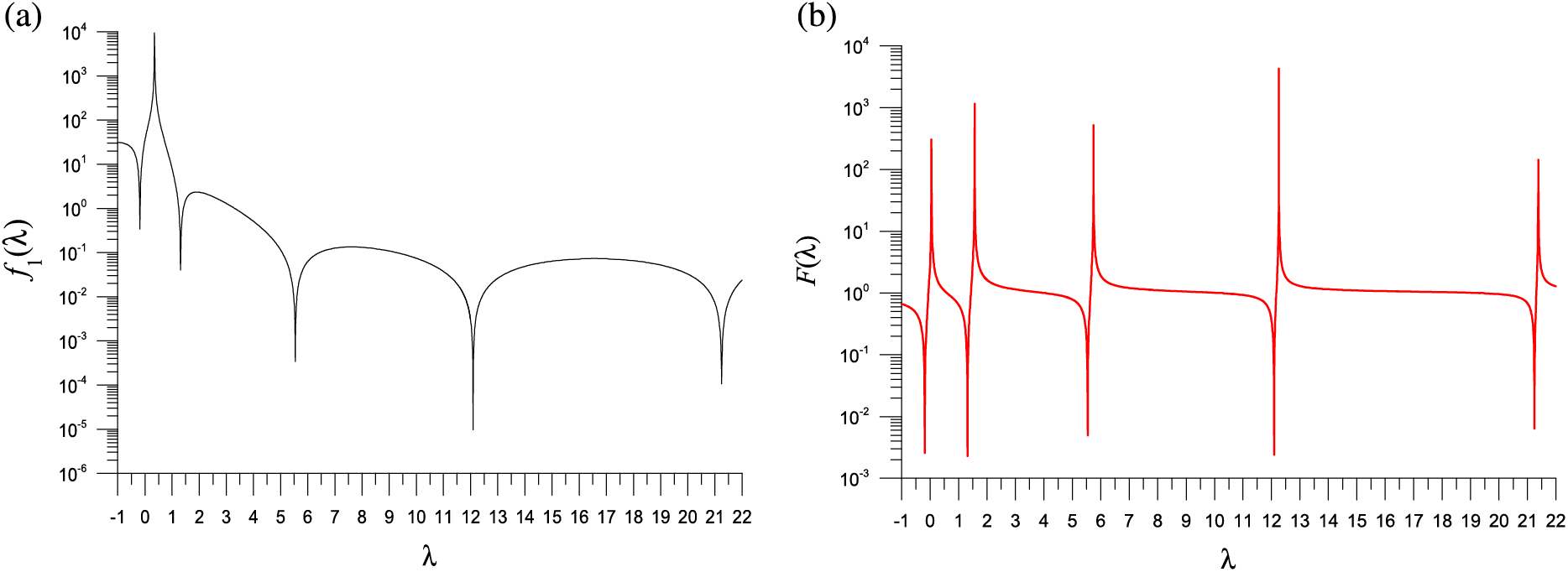
Figure 1: For a generalized eigenvalue problem, showing five minima in a merit function: (a) first method and (b) second method

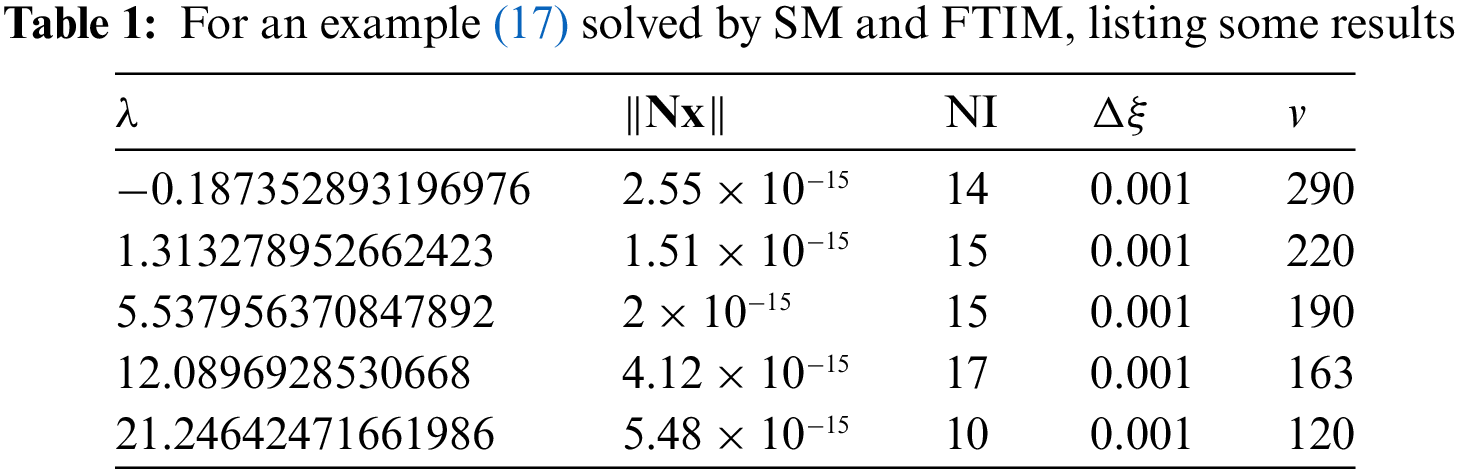
Applying the 1D GSSA to solve this problem, we record the number of iterations (NI) and the number of the computations of f1(λ) (NF). The detailed procedure to determine the precise value of the desired eigenvalue is that we first choose a finer interval [a,b] to only include that eigenvalue, then for each λ∈[a,b] required in the 1D GSSA we compute x from Eq. (13), which is then inserted into Eq. (16) to compute f1(λ). The 1D GSSA can lead to a precise eigenvalue that is minimized in the given interval [a,b].

With [a,b]=[−1,0], we obtain λ=−0.1873528931969765, where NI=73 and NF=74 and ‖Nx‖=7.47×10−15. For other four real eigenvalues we can keep the same efficiency and accuracy by using the 1D GSSA.

We note that the Newton type methods are not suitable for solving the minimization problem in Eq. (16), because those minimal points are very sharp as shown in Fig. 1a.

For a received nonlinear eigenvalue problem, the initial interval [a,b] should be selected large enough to include all real eigenvalues, and then by plotting f1(λ) vs. λ in that interval we can observe several minimal points as shown in Fig. 1a for example (17). These points locate the real eigenvalues approximately, and we apply the 1D GSSA with a smaller interval involving the desired one to compute the eigenvalue very accurately.

2.2 Complex Eigenvalue

The complex eigenvalue is assumed to be

λ=λR+iλI.(18)

Correspondingly, we take

N=N1+iN2,x=z+iw.(19)

Inserting Eqs. (18) and (19) into Eq. (1), yields

[N1−N2N2N1][zw]=0.(20)

Upon letting

X:=[zw],D:=[N1−N2N2N1],(21)

Eq. (20) becomes

D(λR,λI)X=0.(22)

To determine the complex eigenvalue, instead of Eq. (16), we consider

min(λR,λI)∈[a,b]×[c,d]f2(λR,λI):=‖D(λR,λI)X‖≥0.(23)

The first method (FM) seeks the complex eigenvalue by (i) selecting [a,b]×[c,d] and j0; (ii) for each (λR,λI)∈[a,b]×[c,d], required, solving Eqs. (12)–(15) with N replaced by D and x replaced by X; (iii) applying the two-dimensional GSSA (2D GSSA) to Eq. (23).

Both the convergence criteria of the 1D and 2D GSSA are fixed to be 10−15. About the 2D GSSA, one may refer [26].

When λR and λI take values inside a rectangle by (λR,λI)∈[a,b]×[c,d], we can plot ‖DX(λR,λI)‖ vs. (λR,λI) in the rectangle on the eigen-parametric plane. To display the advantage of Eq. (23), we consider a standard eigenvalue problem with

A=[1−112],B=[1001],(24)

whose complex eigenvalues are

λ=32±i32.(25)

We take [a,b]×[c,d]=[1.2,1.9]×[0.5,0.9], and plot f2 over the plane (λR,λI) in Fig. 2, where one minimum point is close to the point (3/2,3/2). When we apply the 2D GSSA to solve this problem, with [a,b]×[c,d]=[1.2,1.9]×[0.5,0.9], we can obtain NI=58, NF=232 and ‖Nx‖=1.54×10−14, and the error of the eigenvalue is 6.51×10−14.

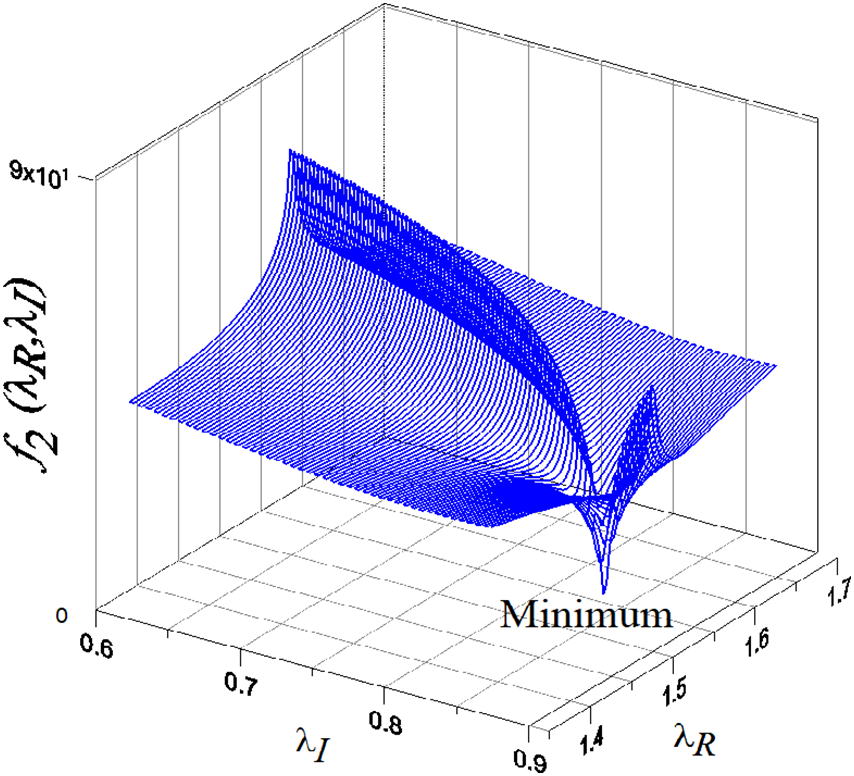
Figure 2: The detection of a complex eigenvalue as a minimal point of a merit function

3  A Simpler Approach to a Nonhomogeneous System

If x is an eigenvector of Eq. (1), then αx, α≠0 is also an eigenvector, which means that the solution x of Eq. (1) is not unique. Therefore, we can impose on Eq. (1) an extra normalization condition:

bTx=1.(26)

We can prove the following result.

Lemma 1. For x≠0 in Eq. (1) being imposed a normalized condition (26), for the eigenvector is unique.

Proof. Suppose that x≠0 and y≠0 are two solutions of Eqs. (1) and (26), and define u=x-y. Taking the difference, yields

Nu=0,(27)

bTu=0.(28)

Combining Eqs. (27) and (28) together yields

[NbT]u=[0n1].(29)

On both sides multiplied by

[NbT]T=[NT b],

we have

[NT b][NbT]u=[NT b][0n1].(30)

Hence, we can derive

(NTN+bbT)u=0.(31)

which leads to u=0 since NTN+bbT is invertible positive definite in view of Eq. (26), and thus

Theorem 1. For x≠0 in Eq. (1) being imposed by a normalized condition (26) for the uniqueness of x∈Rn, a linear equations system to determine x is given by

[N(λ)+bbT]x=b,(32)

where b≠0∈Rn is given.

Proof. Combined Eqs. (1) and (26) together yields an over-determined linear system:

[NbT]x=[0n1](33)

On both sides multiplied by

[NbT]T=[NT b],

we have

[NT b][NbT]x=[NT b][0n1].(34)

Hence, we can derive

(NTN+bbT)x=b.(35)

If the coefficient matrix N is highly ill-conditioned, we can reduce Eq. (35) to Eq. (32), which is easily derived by adding bTxb on both sides of Eq. (1) and from Eq. (26) with bTx=1 being used.

Eq. (35) bears certain similarity to the equations derived in [27,28] for solving ill-posed linear system, where the idea is adding bbT as a regularization of Eq. (1) and b plays the role as a regularization vector.

Eqs. (32) and (16) are the simplest method to find the real eigenvalues of Eq. (1), which is labeled as the second method or a simpler method (SM). It is apparent that Eq. (32) is simpler than Eqs. (12)–(15) used in the first method (FM) to solve the nonzero vector variable x.

In general, the GSSA requires many iterations and the evaluations of merit function to solve the minimization problem. The fictitious time integration method (FTIM) was first coined by Liu et al. [29] to solve a nonlinear equation. Eq. (16) is to be solved by FTIM for finding the real eigenvalues.

Let us define

F(λ):=‖N(λ)x‖,(36)

which is an implicit function of λ. To obtain λ, we need to solve a highly nonlinear scalar equation:

F(λ)=0.(37)

For Eq. (37), Liu et al. [29] developed an iterative scheme:

λk+1=λk+vΔξ1+kΔξF(λk),k=0,1,…,(38)

where Δξ is a fictitious time increment. The iterations in Eq. (38) are terminated if F(λk+1)>F(λk).

Starting from an initial guess λ0 smaller than the desired eigenvalue, Eq. (38) can generate a monotonically increasing sequence of λk, k=1,… to tend to the true eigenvalue. When an initial guess λ0 is larger than the desired eigenvalue, we can take

λk+1=λk−vΔξ1+kΔξF(λk),k=0,1,…,(39)

which makes a monotonically decreasing sequence of λk, k=1,… to tend to the true eigenvalue.

The second method (SM) for determining the real eigenvalue of Eq. (1) is summarized as follows. (i) Select λ0 and b, and give Δξ and v. (ii) Solve Eq. (32) for each required λk. (iii) Apply the FTIM in Eq. (38) for tending to the desired eigenvalue.

We revisit the generalized eigenvalue problem given by Eq. (17) and using the SM. In Fig. 1b, we plot F(λ) with respect to the eigen-parameter in an interval, whose five minimums represent five eigenvalues. The presented merit curve is quite different from that in Fig. 1a obtained by the first method (FM).

With b=(1,0,0,0,0)T, Table 1 lists the eigenvalue, the error ‖Nx‖, the number of iterations (NI), Δξ and v used in the FTIM. The first eigenvalue is very close to that obtained by the first method in Section 2.1. The accuracy of the SM is slightly better than the FM with a smaller error of ‖Nx‖. Moreover, NI is saving about five times.

Theorem 2. For x≠0 in Eq. (1) being imposed by a normalized condition (26) for the uniqueness of x∈Cn, if λ is a complex eigenvalue, a linear equations system to determine x can be derived as follows:

[N1+bbT−N2N2N1+bbT][uv]=[b0n],(40)

where

λ=λR+iλI,N=N1+iN2,x=u+iv.(41)

Proof. Inserting Eq. (41) into Eq. (32), yields

(N1+bbT+iN2)(u+iv)=b.(42)

Equating the real and imaginary parts of Eq. (42), we have

(N1+bbT)u−N2v=b,N2u+(N1+bbT)v=0,(43)

which can be recast to that in Eq. (40).

When x is solved from Eq. (40), we can employ the minimization in Eq. (23) by picking up the complex eigenvalue with the aid of 2D GSSA.

We revisit the standard eigenvalue problem given by Eq. (24) by using the SM with b=(1,1)T and ε=10−15 for the 2D GSSA. With [a,b]×[c,d]=[1.2,1.9]×[0.5,0.9], we can obtain NI=73 and ‖Nx‖=7.22×10−16, and the error of the eigenvalue is 4.44×10−16. The SM is more accurate than the FM.

To compare with the Newton method, we supplement Eq. (1) by

‖x‖=1,(44)

which is a normalized condition. Letting xn+1=λ, yields the following nonlinear equations with dimension m=n+1:

N(xm)x=0,(45)

x12+…+xn2−1=0.(46)

At the k-th step the Jacobian matrix reads as

Jk=[N(xmk)N′(xmk)xk2(xk)T0   ].(47)

Then the Newton iteration method is given by

[xk+1xmk+1]=[xk+1xmk+1]−Jk−1[N(xmk)xk‖xk‖2−1].(48)

The iteration is terminated if it converges with a given criterion ε=10−15.

In Table 2, we list the results computed from the Newton method, where the initial guess is x0=1 and λ0=c0.

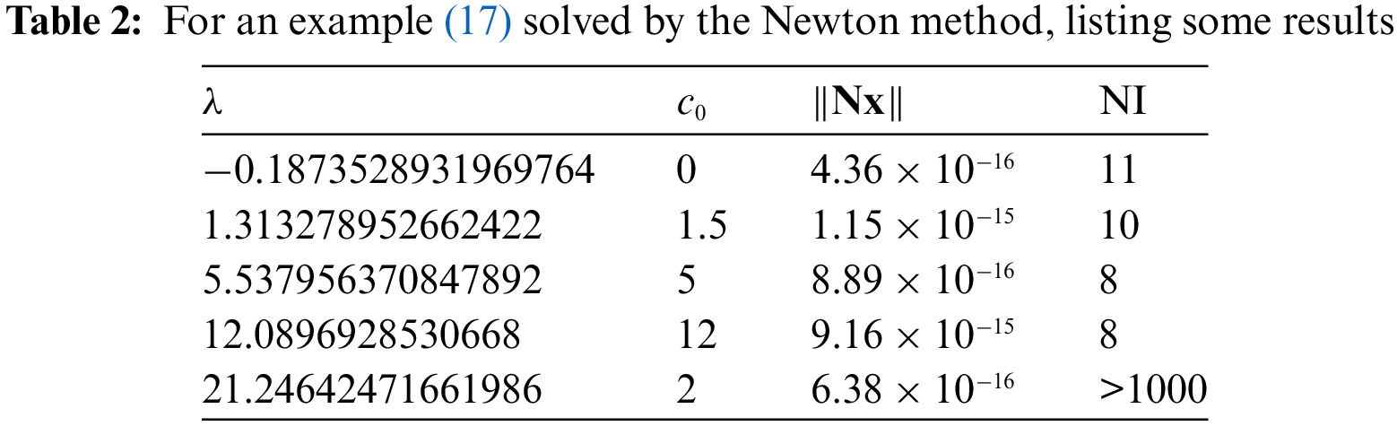
We can observe that c0 must be chosen to close the exact eigenvalue; otherwise, it converges very slowly as that for the last eigenvalue.

To improve the performance, we can combine the Newton method to the SM, and solve Eqs. (32) and (26) by the following iteration:

[xk+1xmk+1]=[xkxmk]−[N(xmk)+bbTN′(xmk)xkbT0]−1[N(xmk)xk+b⋅xkb−bb⋅xk−1].(49)

The iteration is terminated if the given convergence criterion ε=10−15 is fulfilled.

In Table 3, we list the results computed from the SM and Newton method, where b=(1,0,…,0)T and the initial guess is x0=1 and λ0=c0.

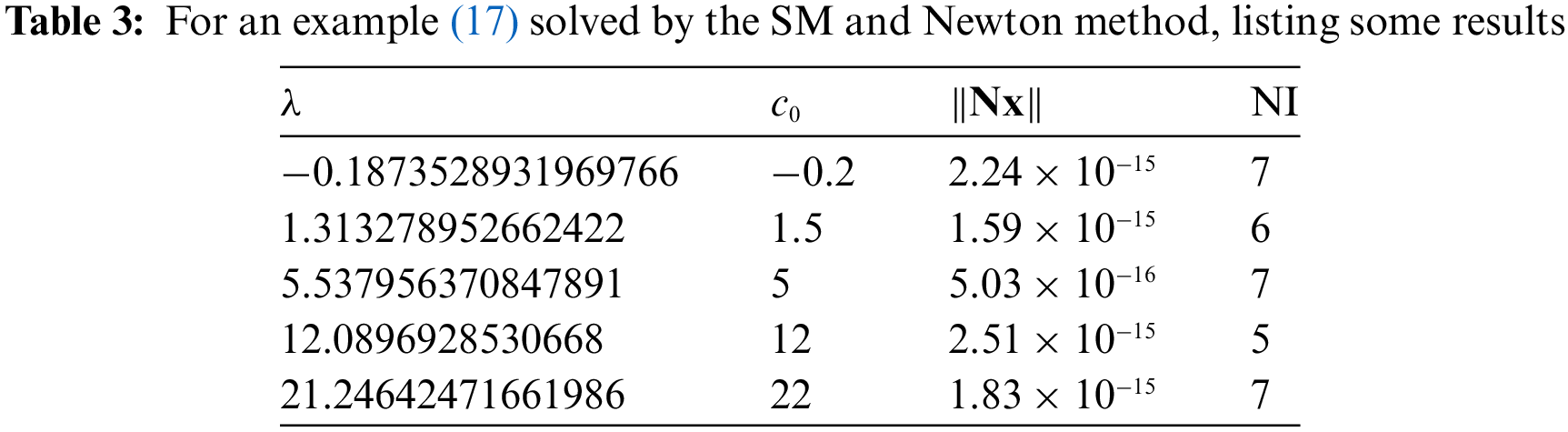
Upon comparing Table 3 with Table 2, it is obvious that the combination of the simpler method (SM) to the Newton iteration outperforms the original Newton method.

Remark 1. Even the proofs of Theorems 1 and 2 are simple and straightforward, they are crucial for the developments of the proposed numerical methods for effectively and accurately solving the nonlinear eigenvalue problems. Eq. (49) as an application of Theorem 1 is a very effective combination of the SM and Newton method to solve nonlinear eigenvalue problems.

4  Examples of Nonlinear Eigenvalue Problems

Example 1. Consider

N(λ)x=(λ2M+λC+K)x=0,(50)

where

M=[060060001],C=[1−602−70000],K=I3.(51)

We apply the 1D GSSA to solve this problem. With [a,b]=[0,0.1], we obtain λ=0.04080314176866114, where NI=68 and NF=69. ‖Nx‖=8.62×10−16 is obtained. With [a,b]=[0.6,0.8], we obtain λ=0.7425972620277175, where NI=70, NF=71 and ‖Nx‖=0. Let λ=μ and we can derive

N1=[(μR2−μI2)2−4μR2μI2]M+μRC+K,N2=4μRμI(μR2−μI2)M+μIC.(52)

There are totally 24 eigenvalues as shown in Fig. 3a, which are computed by the detecting method based on 2D GSSA.

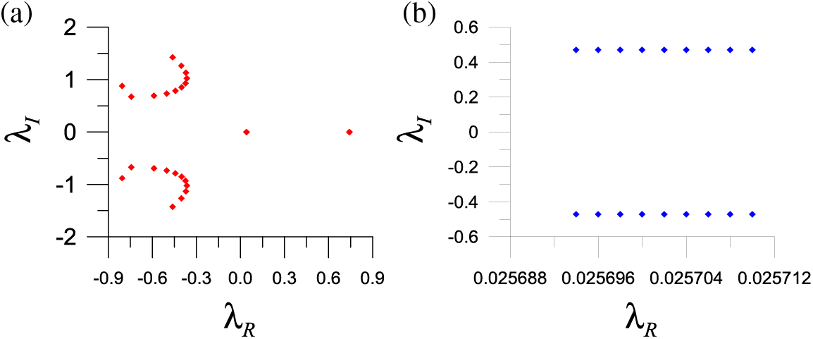
Figure 3: For the distribution of (a) example 1 with 24 eigenvalues and (b) example 3 with 18 eigenvalues

In Eq. (50), if λ is replaced by λ, there exist four real eigenvalues 1/3, 1/2, 1, ∞ and two imaginary eigenvalues ±i as shown in [4].

With b=(1,1,1)T, we plot F(λ) in Fig. 4 with respect to the eigen-parameter, of which two minimums represent two real eigenvalues.

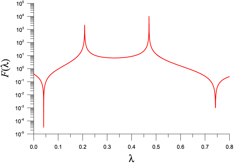
Figure 4: For a nonlinear eigenvalue problem of example 1 solved by SM, showing two minimums in a function F used in the FTIM

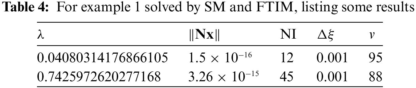
Table 4 lists the eigenvalue, the error ‖Nx‖, the number of iterations (NI), Δξ and v used in the FTIM.

Example 2. Next, we consider [8]

N(λ)x=[A+exp⁡(−λ)B−λI3]x=0,(53)

where

A=[010001−a3−a2−a1],B=[000000−b3−b2−b1].(54)

It describes a time-delay system.

We take a1 = 1.5, a2 = 1, a3 = 0.5 and b1 = 0.3, b2 = 0.2, b3 = 0.1, and there exist four complex eigenvalues. Through some manipulations, we find that

N1=(λR,λI)=A+exp⁡(−λR)cos⁡λIB−λRI3,N2=(λR,λI)=−exp⁡(−λR)sin⁡λIB−λII3.(55)

When we apply the 2D GSSA to solve this problem, with [a,b]×[c,d]=[−1.5,1.5]×[0,10] and j0 = 2, we obtain NI=78, NF=312 and ‖Nx‖=4.96×10−16. The complex eigenvalue is λ=−0.3208498325636319±i0.6608850649667835, and the corresponding complex eigenvector is x1=−0.5944815593616035−i1.224510484674573, x2=1 and x3=−0.3208498325636320−i0.6608850649667830. With [a,b]×[c,d]=[−1.5,−1.4]×[0.9,1.1] and j0 = 2, we obtain NI=70, NF=280 and ‖Nx‖=8.95×10−16. The complex eigenvalue is λ=−1.422926059141503±i1.035178169828797, and the corresponding complex eigenvector is x1 = −0.4595550672255327−i0.3343261375879888, x2=1, and x3=−1.422926059141503+i1.035178169828797.

By taking the parameters of ai, bi, i = 1, 2, 3 as that listed in [8,30], there exists a double non-semi simple eigenvalue 3πi. With [a,b]×[c,d]=[−10−15,10−15]×[9.42,9.45] and j0 = 6, we obtain NI=60, NF=240 and ‖Nx‖=3.97×10−15. The eigenvalue obtained is very close to 3πi with an error 6.17×10−10. To detect the imaginary eigenvalue, we can also use the 1D GSSA with [c,d]=[9.42,9.43] and j0 = 6; we can obtain NI=56, NF=60, ‖Nx‖=1.78×10−15 and with an error 4.66×10−10 of the obtained eigenvalue.

Example 3. From [8]

N(λ)=λ3A3+λ2A2+A0,(56)

where

A3=[−4312−17−1101−13],A2=[2−61−222117−11],A0=[−16−47−14713687].(57)

We can derive

N1(λR,λI)=(λR3−3λRλI2)A3+(λR2−λI2)A2+A0,N2(λR,λI)=(3λR2λI−λI3)A3+2λRλIA2.(58)

By applying the 2D GSSA to solve this problem with [a,b]×[c,d]=[0.01,0.03]×[0.4,0.5] and j0=6, we obtain NI=68, NF=272 and ‖Nx‖=3.595×10−15. While the complex eigenvalue is λ=0.02570242595103067+i0.4701394321627314, the complex eigenvector is x1 = −0.1802298005308327+i0.6067208490359938, x2=0.3535853100582456−i1.158223781021044, and x3=−0.3638331326048661+i. There are totally 18 eigenvalues as shown in Fig. 3b. Notice that the eigenvalue λ = 0.0257 + i0.4701 provided in [8] leads to a much larger error with ‖Nx‖=1.65×10−3.

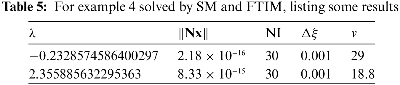
Example 4. We consider

N(λ)=λ2A2+λA1+A0,(59)

where

A2=[−4312−17−1101−13],A1=[2−61−222117−11],A0=[−16−47−14713687].(60)

We apply the SM to solve this problem with b=(0,1,0)T and ε=10−15. In Fig. 5, with respect to the eigen-parameter in an interval, two minimums represent two real eigenvalues.

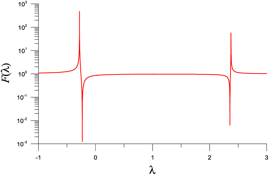
Figure 5: For a nonlinear eigenvalue problem of example 4 solved by SM, showing two minima in a function F used in the FTIM

Table 5 lists the eigenvalue, the error ‖Nx‖, the number of iterations (NI), Δξ and v used in the FTIM.

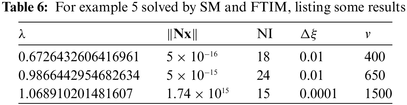
Example 5. This example is Example 6.2 of [31], and we have a quadratic eigenvalue problem (3) with

M=c11Im⊗M∼+c12M∼⊗Im,C=c21Im⊗C∼+c22C∼⊗ImK=c31Im⊗K∼+c32K∼⊗Im,(61)

where

M∼=16(4Im+B+BT),C∼=B−BT,K∼=B+BT−2Im,B=[00⋯010⋯0⋱⋱⋱⋮…010].(62)

By taking m = 5, we have n = 25, and we take c11 = 1, c12 = 1.3, c21 = 0.1, c22 = 1.1, c31 = 1 and c32 = 1.2.

We apply the SM to solve this problem with b=(1,…,1)T and ε=10−15. In Fig. 6, with respect to the eigen-parameter in an interval, three minimums represent three real eigenvalues.

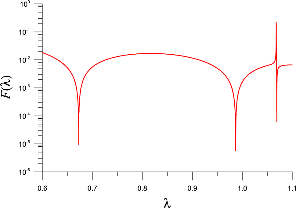
Figure 6: For a nonlinear eigenvalue problem of example 5 solved by SM, showing three minima in a function F used in the FTIM

Table 6 lists the eigenvalue, the error ‖Nx‖, the NI, Δξ and v used in the FTIM. The last eigenvalue in Table 6 can be obtained from the FTIM (39).

In Table 7, we list the results computed from the Newton method, where the initial guess is x0=1 and λ0=c0.

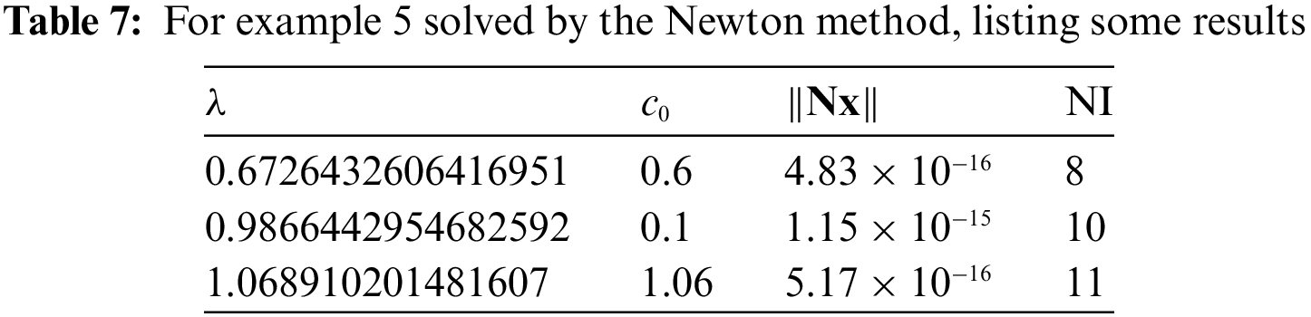
We can observe that c0 must be chosen to close the exact eigenvalue; otherwise, it converges very slowly as that for the first and third eigenvalues.

In Table 8, we list the results computed from the Newton method, where b=1 and the initial guess is x0=1 and λ0=c0.

Upon comparing Table 8 to Table 7, the performance is improved by combining SM to the Newton method.

Example 6. As a practical application, we consider a five-story shear building with [32]

M=[140000001200000000000012000000100]kipg,K=[800−400000−400600−200000−200400−200000−200300−100000−100100]kipin.(63)

We take n = 5 and plot ‖f1(ω)‖ vs. ω in Fig. 7a, where we can observe five minimal points. Starting from [a,b]=[0,1] and under a convergence criterion 10−15, with NI = 73 and NF = 74, ω2=0.203999161269661 is obtained and ‖Kx−ω2Mx‖=1.27×10−13 is obtained, where x is solved from Eqs. (12)–(15) with j0 = 1 with the first mode being shown in Fig. 7b at the first column.

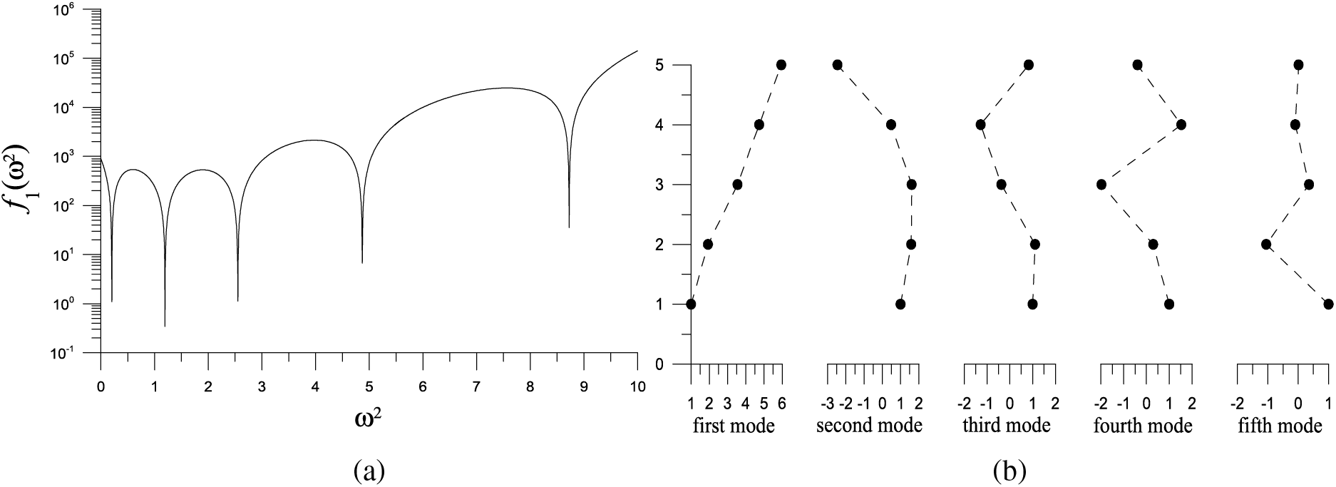
Figure 7: For example 6 of a five-degree MK system, (a) showing five minima in a merit function, and (b) displaying the five vibration modes

Starting from [a,b]=[1,2] and with NI = 73 and NF = 75, ω2=1.195924448669029 is obtained and ‖Kx−ω2Mx‖=1.27×10−13 is obtained, with the second mode being shown in Fig. 7b at the second column.

Starting from [a,b]=[2,3] and with NI = 73 and NF = 74, ω2=2.55144529001161 is obtained and ‖Kx−ω2Mx‖=3.18×10−13 is obtained, with the third mode being shown in Fig. 7b at the third column.

Starting from [a,b]=[4,5] and with NI = 72 and NF = 74, ω2=4.870842516791812 is obtained and ‖Kx−ω2Mx‖=5.72×10−13 is obtained, with the fourth mode being shown in Fig. 7b at the fourth column.

Starting from [a,b]=[8,9] and under a convergence criterion 10−15, with NI = 71 and NF = 73, ω2=8.725407630876937 is obtained and ‖Kx−ω2Mx‖=3.98×10−11 is obtained, where x is solved from Eqs. (12)–(15) with j0 = 1, and the fifth mode is shown in Fig. 7b at the fifth column.

5  Conclusions

This study proposes two simple approaches to solve the nonlinear eigenvalue problems, which directly implement a normalization condition for the uniqueness of the eigenvector into the eigen-equation. When the eigen-parameter runs in a desired range, the curve or surface for real and complex eigenvalues reveals local minimums of the constructed merit functions. In the merit function, the vector variable is solved from the nonhomogeneous linear system, which is available by reducing the eigen-equation by one dimension less and moving the normalized component to the right side. It is possible to quickly obtain the real and complex eigenvalues using 1D and 2D golden section search algorithms to solve the resultant minimization problems. The second method is simpler than the first by inserting the normalization condition into the eigen-equation. From the resulting nonhomogeneous linear system, the fictitious time integration method (FTIM) computes the real eigenvalues faster, which saves computation costs compared to the GSSA. The combination of the simpler method with the Newton iteration outperforms the original Newton method. Combining the simpler method to the Newton iteration without using the extra parameters is also better than the FTIM. It can obtain highly precise eigenvalues and eigenvectors very fast.

Acknowledgement: The authors would like to thank the National Science and Technology Council, Taiwan, for their financial support (Grant Number NSTC 111-2221-E-019-048).

Funding Statement: The corresponding authors would like to thank the National Science and Technology Council, Taiwan for their financial support (Grant Number NSTC 111-2221-E-019-048).

Author Contributions: The authors confirm contribution to the paper as follows: study conception and design: Chein-Shan Liu; data collection: Jian-Hung Shen; analysis and interpretation of results: Yung-Wei Chen; draft manuscript preparation: Chung-Lun Kuo and all authors reviewed the results and all approved the final version of the manuscript.

Availability of Data and Materials: Not applicable.

Conflicts of Interest: The authors declare that they have no conflicts of interest to report regarding the present study.

References

1. Betcke, T., Higham, N. J., Mehrmann, V., Schröder, C., Tisseur, F. (2013). NLEVP: A collection of nonlinear eigenvalue problems. ACM Transactions on Mathematical Software, 39(2), 1–28. https://doi.org/10.1145/2427023.2427024 [Google Scholar] [CrossRef]

2. Qian, J., Lin, W. W. (2007). A numerical method for quadratic eigenvalue problems of gyroscopic systems. Journal of Sound and Vibration, 306(1–2), 284–296. https://doi.org/10.1016/j.jsv.2007.05.009 [Google Scholar] [CrossRef]

3. Chen, C., Ma, C. (2019). An accelerated cyclic-reduction-based solvent method for solving quadratic eigenvalue problem of gyroscopic systems. Computers & Mathematics with Applications, 77(10), 2585–2595. https://doi.org/10.1016/j.camwa.2018.12.040 [Google Scholar] [CrossRef]

4. Tisseur, F., Meerbergen, K. (2001). The quadratic eigenvalue problem. SIAM Review, 43(2), 235–286. https://doi.org/10.1137/S003614450038198 [Google Scholar] [CrossRef]

5. Higham, N. J., Kim, H. M. (2001). Solving a quadratic matrix equation by Newton’s method with exact line searches. SIAM Journal on Matrix Analysis and Applications, 23(2), 303–316. https://doi.org/10.1137/S089547989935097 [Google Scholar] [CrossRef]

6. Meerbergen, K. (2009). The quadratic Arnoldi method for the solution of the quadratic eigenvalue problem. SIAM Journal on Matrix Analysis and Applications, 30(4), 1463–1482. https://doi.org/10.1137/07069273X [Google Scholar] [CrossRef]

7. Hammarling, S., Munro, C. J., Tisseur, F. (2013). An algorithm for the complete solution of quadratic eigenvalue problems. ACM Transactions on Mathematical Software, 39(3), 1–19. https://doi.org/10.1145/2450153.2450156 [Google Scholar] [CrossRef]

8. Jarlebring, E. (2012). Convergence factors of Newton methods for nonlinear eigenvalue problems. Linear Algebra and its Applications, 436(10), 3943–3953. https://doi.org/10.1016/j.laa.2010.08.045 [Google Scholar] [CrossRef]

9. Mehrmann, V., Voss, H. (2004). Nonlinear eigenvalue problems: A challenge for modern eigenvalue methods. GAMM Mitteilungen, 27(2), 121–152. https://doi.org/10.1002/gamm.201490007 [Google Scholar] [CrossRef]

10. Betcke, M. M., Voss, H. (2008). Restarting projection methods for rational eigenproblems arising in fluid-solid vibrations. Mathematical Modelling and Analysis, 13(2), 171–182. https://doi.org/10.3846/1392-6292.2008.13.171-182 [Google Scholar] [CrossRef]

11. Hochstenbach, M. E., Sleijpen, G. L. (2008). Harmonic and refined Rayleigh-Ritz for the polynomial eigenvalue problem. Numerical Linear Algebra with Applications, 15(1), 35–54. https://doi.org/10.1002/nla.562 [Google Scholar] [CrossRef]

12. Xiao, J., Zhou, H., Zhang, C., Xu, C. (2017). Solving large-scale finite element nonlinear eigenvalue problems by resolvent sampling based Rayleigh-Ritz method. Computational Mechanics, 59, 317–334. https://doi.org/10.1007/s00466-016-1353-4 [Google Scholar] [CrossRef]

13. Chiappinelli, R. (2018). What do you mean by “nonlinear eigenvalue problems”? Axioms, 7(2), 39. https://doi.org/10.3390/axioms7020039 [Google Scholar] [CrossRef]

14. Meirovitch, L. (1986). Elements of vibrational analysis, 2nd edition. New York: McGraw-Hill. [Google Scholar]

15. Smith, H. A., Singh, R. K., Sorensen, D. C. (1995). Formulation and solution of the non-linear, damped eigenvalue problem for skeletal systems. International Journal for Numerical Methods in Engineering, 38(18), 3071–3085. https://doi.org/10.1002/nme.1620381805 [Google Scholar] [CrossRef]

16. Osinski, Z. (1998). Damping of vibrations. Rotterdam, Netherlands: A.A. Balkema. https://doi.org/10.1201/9781315140742 [Google Scholar] [CrossRef]

17. Sadet, J., Massa, F., Tison, T., Turpin, I., Lallemand, B. et al. (2021). Homotopy perturbation technique for improving solutions of large quadratic eigenvalue problems: Application to friction-induced vibration. Mechanical Systems and Signal Processing, 153, 107492. https://doi.org/10.1016/j.ymssp.2020.107492 [Google Scholar] [CrossRef]

18. Hashemian, A., Garcia, D., Pardo, D., Calo, V. M. (2022). Refined isogeometric analysis of quadratic eigenvalue problems. Computer Methods in Applied Mechanics and Engineering, 399, 115327. https://doi.org/10.1016/j.cma.2022.115327 [Google Scholar] [CrossRef]

19. Sadet, J., Massa, F., Tison, T., Talbi, E., Turpin, I. (2022). Deep Gaussian process for the approximation of a quadratic eigenvalue problem application to friction-induced vibration. Vibration, 5(2), 344–369. https://doi.org/10.3390/vibration5020020 [Google Scholar] [CrossRef]

20. Lee, S., Bathe, K. J. (2022). Solution of the generalized eigenvalue problem using overlapping finite elements. Advances in Engineering Software, 173, 103241. https://doi.org/10.1016/j.advengsoft.2022.103241 [Google Scholar] [CrossRef]

21. Hari, V. (2022). On the quadratic convergence of the complex HZ method for the positive definite generalized eigenvalue problem. Linear Algebra and its Applications, 632, 153–192. https://doi.org/10.1016/j.laa.2021.08.022 [Google Scholar] [CrossRef]

22. Dan, J., Geirnaert, S., Bertrand, A. (2022). Grouped variable selection for generalized eigenvalue problems. Signal Processing, 195, 108476. https://doi.org/10.1016/j.sigpro.2022.108476 [Google Scholar] [CrossRef]

23. Alkilayh, M., Reichel, L., Ye, Q. (2023). A method for computing a few eigenpairs of large generalized eigenvalue problems. Applied Numerical Mathematics, 183, 108–117. https://doi.org/10.1016/j.apnum.2022.08.018 [Google Scholar] [CrossRef]

24. Liu, C. S., Kuo, C. L., Chang, C. W. (2022). Free vibrations of multi-degree structures: Solving quadratic eigenvalue problems with an excitation and fast iterative detection method. Vibration, 5(4), 914–935. https://doi.org/10.3390/vibration5040053 [Google Scholar] [CrossRef]

25. Golub, G. H., van Loan, C. F. (2013). Matrix computations. Maryland: The John Hopkins University Press. [Google Scholar]

26. Rani, G. S., Jayan, S., Nagaraja, K. V. (2019). An extension of golden section algorithm for n-variable functions with MATLAB code. IOP Conference Series: Materials Science and Engineering, 577(1), 012175. https://doi.org/10.1088/1757-899X/577/1/012175 [Google Scholar] [CrossRef]

27. Liu, C. S., Hong, H. K., Atluri, S. N. (2010). Novel algorithms based on the conjugate gradient method for inverting ill-conditioned matrices, and a new regularization method to solve ill-posed linear systems. Computer Modeling in Engineering & Sciences, 60(3), 279–308. https://doi.org/10.3970/cmes.2010.060.279 [Google Scholar] [CrossRef]

28. Liu, C. S. (2012). Optimally scaled vector regularization method to solve ill-posed linear problems. Applied Mathematics and Computation, 218(21), 10602–10616. https://doi.org/10.1016/j.amc.2012.04.022 [Google Scholar] [CrossRef]

29. Liu, C. S., Atluri, S. N. (2008). A novel time integration method for solving a large system of non-linear algebraic equations. Computer Modeling in Engineering & Sciences, 31(2), 71–83. https://doi.org/10.3970/cmes.2008.031.071 [Google Scholar] [CrossRef]

30. Jarlebring, E., Michiels, W. (2010). Invariance properties in the root sensitivity of time-delay systems with double imaginary roots. Automatica, 46(6), 1112–1115. https://doi.org/10.1016/j.automatica.2010.03.014 [Google Scholar] [CrossRef]

31. Mehrmann, V., Watkins, D. (2001). Structure-preserving methods for computing eigenpairs of large sparse skew-Hamiltonian/Hamiltonian pencils. Journal on Scientific Computing, 22(6), 1905–1925. https://doi.org/10.1137/S1064827500366434 [Google Scholar] [CrossRef]

32. Berg, G. V. (1998). Elements of structural dynamics. New Jersey: Prentice-Hall. [Google Scholar]

Appendix

In this appendix, we demonstrate the computer code to obtain the coefficient matrix [cij] from [nij] by

Do i=1:n0,

k=0,

Do j=1:n,

If j=j0 next j,

k=k+1,

cik=nij,

Enddo of j,

Enddo of i.(A1)

If (y1,…,yn0) in Eq. (14) can be obtained by a suitable linear solver, x=(x1,…,xn)T is computed by

k=0,

Do j=1:n,

If j=j0 xj=1, next j,

k=k+1,

xj=yk.(A2)