Toward Improved Accuracy in Quasi-Static Elastography Using Deep Learning

1  Introduction

Elastography is a non-invasive medical imaging technique to map the elastic properties and stiffness of soft tissues. It has been prevalent in clinical medicine and applied to diagnose tumorous diseases, including breast and thyroid cancers [1–4]. For the static elastography [1,5–7], the tissue deformation throughout the region of interest (ROI) can be obtained by applying quasi-static uniaxial compression [8,9]. Since the shear modulus or Young’s modulus is inversely proportional to the strain for a linear elastic material subject to the uniaxial compression, the strain images can be used to assess the stiffness distribution of the ROI [10]. However, strain imaging is usually very noisy and cannot quantify the elastic property distribution of soft tissues. Alternatively, we can solve the inverse problem in elasticity to identify the elastic property distribution of soft tissues. Typically, the inverse problem in elasticity is posed as a constrained optimization problem where the equilibrium equations associated with linear elastic solids should be satisfied [11–13]. In every optimization step, the forward problem in elasticity needs to be solved to update the displacement field under the current estimation of the elastic property distribution, and solving the forward problem requires boundary conditions. In elastography, we are merely interested in a sub-region of the entire organ. Thus, the exact boundary conditions cannot be determined. Moreover, the iterative inverse approach is computationally intensive. Thus, the real-time display of the reconstructed results cannot be realized. Most importantly, since it is unrealistic to eliminate noise from measured data, the reconstructed elastic property distribution is always influenced by noise and cannot be recovered to its exact distribution.

In the past decade, the rapid progress in machine learning (ML) or deep learning (DL) provides state-of-the-art techniques to solve the parameter identification problem. Especially for the applications of elasticity imaging, great efforts are made to make the ML and DL powerful tools with high accuracy and computational efficiency [14–18]. A variety of deep learning network architectures are used for material parameter identification from different perspectives [19–22], such as conditional Generative Adversarial Networks [14], physics-informed neural network [19], and convolutional neural network [20]. In the framework of DL, we are merely concerned with image-to-image translation. Thus, the requirement of the boundary conditions in the optimization-based approaches can be circumvented [18]. Further, with well-trained DL models, the reconstructed elastic property distribution can be reconstructed and displayed very fast. Therefore, there is great potential to develop novel and real time elastography techniques based on DL in clinical medicine. It should be noted that there have been a few studies on elastography based on DL models. Patel et al. applied Convolutional Neural Networks (CNN) models to directly classify malignant and benign tumors from displacement images in order to avoid solving for and analyzing the elastic modulus images [18]. As a result, the location and shape of the tumors cannot be determined. This is not beneficial for the cancer ablation treatment in which the tumors should be accurately located. Ni et al. have used the conditional Generative Adversarial Networks (cGAN) model to solve the inverse problem in elasticity to identify the nonhomogeneous elastic property distribution of solids [14]. However, this work merely shows the proof of concept with simulated data. Besides, the strain field is usually very noisy, which can contribute errors to the solution of the inverse elasticity problem. Therefore, the feasibility of the DL model in elastography should be further examined.

In this paper, we apply the cGAN to solve the inverse problem in elasticity and characterize the shear modulus distribution of soft tissues. In the training process, we utilize the simulated data acquired from finite element simulation [23] instead of the scarce clinical dataset in typical studies [24,25]. In the testing process, we will utilize both the noisy simulated data and experimental data to test the feasibility and reliability of the proposed approach. In order to make the DL model more robust to noise, we also attempt to recover the exact elastic property distribution with a noisy training displacement field. The reconstructed shear modulus distribution acquired from the DL model is also compared with the optimization-based inverse approach.

This work is organized as follows: In Methods Section, we will discuss how to apply the cGAN model to solve the inverse problem in elasticity. In Results Section, we validate the quality of the shear modulus reconstructions with several typical numerical and experimental examples. Observations are discussed and analyzed in Discussion Section. In the end, we summarize our findings in Conclusion Section.

2  Methods

In this paper, we employ a Deep Learning (DL) methodology to effectively characterize the distribution of elastic properties in soft solids using full-field displacement fields. The foundation of this method lies in utilizing displacement field data derived from finite element simulations as the training dataset, with the shear modulus distribution as the target parameter. To validate the efficacy of our proposed DL approach, we leverage both simulated finite element data and a collection of experimental datasets. The accuracy of the reconstructed shear modulus distribution is then juxtaposed against results obtained through the optimization-based inverse method (OP) which is based on the adjoint method [26,27]. For a concise overview of the OP technique, please refer to Part B in the supplementary materials.

2.1 cGAN-Based DL Method

A GAN comprises two fundamental components: a generator and a discriminator. The generator’s purpose is to craft synthetic data from unknown distributions, while the discriminator is tasked with distinguishing counterfeit samples from authentic ones. These two networks engage in a dynamic, zero-sum training process, continually challenging each other. A specialized variant of the GAN, known as a conditional GAN (cGAN), introduces a conditional framework. Here, both the generator and discriminator factor in auxiliary information, enabling the cGAN model to discern specific patterns. Notably, cGANs find extensive utility in image translations, as evidenced by applications and investigations [28–30].

In our current study, we employ a cGAN-based Pix2Pix model for effecting translations from displacement fields to material distributions. For the generator and discriminator roles, we adopt the U-net architecture and PatchGAN, respectively [29,31], as depicted in Fig. 1. Given the substantial body of work that delves into the theoretical and structural aspects of cGANs [29,32], we refrain from an exhaustive discussion herein. Our focus centers on the generator, which fabricates synthetic shear modulus distributions based on the input displacement field. Simultaneously, the discriminator discerns these fabricated distributions from authentic shear modulus distributions originating from the same displacement field. The training dataset stems from finite element simulations, and our model’s efficacy is assessed using both simulated and experimental datasets. A schematic illustration of the cGAN-based displacement-modulus mapping model can be found in Fig. 1.

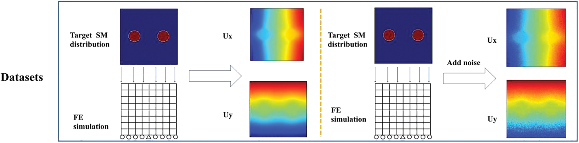
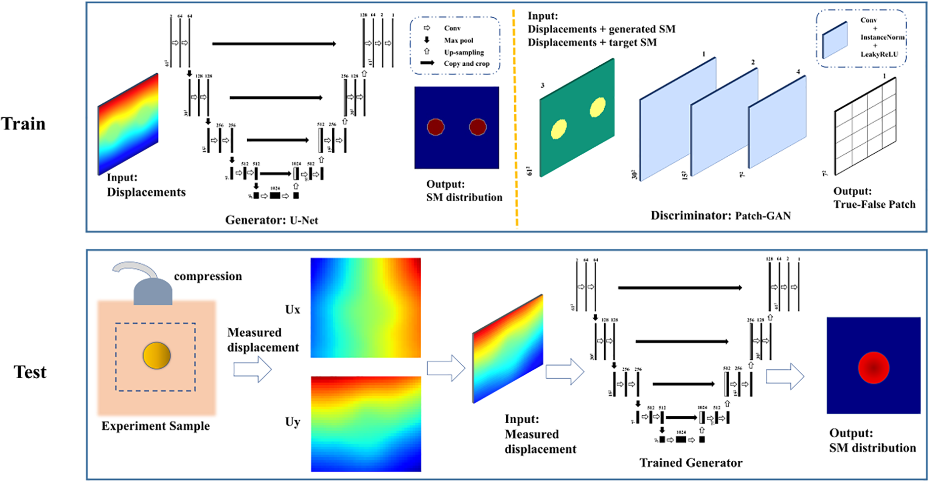
Figure 1: Flowchart of the cGAN-based inverse scheme: The training data for our DL model was generated through finite element simulation, and we utilized a cGAN structure to train the model. Our trained DL model will subsequently be tested using experimental data

The adopted generator encoder-decoder U-net structure is shown in Fig. 2. Inspired by [29], the objective function to be minimized is written as:

G∗=argminG maxDLcGAN(G,D)+λLL1(G)(1)

where LcGAN(G,D)=Ex,y[log⁡D(x,y)]+Ex[log⁡(1−D(x,G(x))] and LL1(G)=Ex,y[‖y−G(x)‖1]. E denotes the expectation in statistics, x is the input displacement image with channel 61 × 61 × 2 since both the axial and lateral displacement components are involved in the training process and the domain of interest is discretized by 61 × 61 nodes. y is the associated target shear modulus (SM) distribution image with channel 61 × 61 × 1. G(x) are the generated shear modulus distribution image by the generator G from x. D(x,y) and D(x,G(x)) represent the discrimination of true and fake samples by the discriminator D, respectively. In addition, we also use the L1 loss term for the U-net for contributing to the generation of fake samples, where λ is the weight of the L1 loss. In this study, we conducted a search for λ values ranging from 0 to 100, and based on our results, we recommend setting λ to 60.

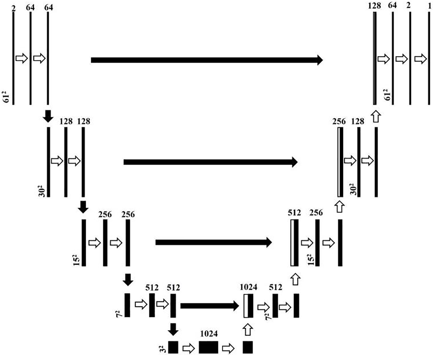
Figure 2: The structure of the adopted U-net translating the displacement input (with channel 61 × 61 × 2) to the SM output (with channel 61 × 61 × 1)

The cGAN models are Implemented with Pytorch1.7.1, CUDA11.0, Nvidia RTX2080. The Adam optimizer is adopted to train the cGAN model, with a learning rate of 0.002 and momentum parameters β1 = 0.5, β2 = 0.999.

2.2 Sample Generation

The training data is generated from the finite element simulation. The governing equation is given by:

∇⋅σ=0onΩ(2)

u=u∘     onΓu(3)

σ⋅n=t∘  onΓt(4)

In Eqs. (2)–(4), Γu and Γt denote the displacement and traction boundaries, respectively. The prescribed displacement and traction are represented by u∘ and t∘, respectively. Γu∪Γt=∂Ω constitutes the entire boundary of the problem domain Ω, and Γu∩Γt=∅ without overlapping. The soft tissue is assumed to be incompressible and linear elastic solid. The stress tensor σ can be expressed in terms of the strain tensor ε, shear modulus μ, identity tensor I and hydrostatic pressure p for an incompressible linear elastic material:

σ=2με+pI(5)

Thus, we merely need to reconstruct the shear modulus distribution herein. To generate the simulated datasets, we use the target shear modulus distribution throughout the problem domain and solve for the corresponding displacement field using linear finite element method. In this study, the shear modulus distribution is considered as the circular inclusions embedded in the square domain. The location and size of the circular inclusions vary among different samples. To better simulate the practical situations, we set the shear modulus of inclusions to the range of 2–200 kPa, while the shear modulus of the background is 1 kPa. The radius of the circular inclusions varies between 0.1 and 0.2 mm, and the centroid of each inclusion is appropriately positioned inwards within the square domain to prevent any penetration beyond its boundaries. A uniform pressure of 0.1 kPa is applied on the top edge of the square domain, while the y-direction displacement of the bottom edge is fixed, and the x-direction displacement of the center of the bottom edge is also fixed. We assume the small deformation theory for all samples, as the global strain was within 5% for each of the samples.

Since the experimental or clinical data is usually noisy, we add noise to the simulated displacement field in training to reduce the impact of noise on the reconstructed results. The noise level is defined by:

noise level=∑i=1NN(u¯i−ui)2∑i=1NNu¯i2×100%(6)

where NN is the total number of the finite element nodes in the domain of interests. u¯i and ui are the nodal exact and noisy displacement values, respectively. We will also utilize the noisy dataset at different noise levels for training and testing.

Note that, for the sake of convenience, the naming convention for the test datasets and trained models is as following: For the test datasets, the name will be “TestData (xx%, N)”, xx% is the noise level of the test data and N is the target number of the inclusions of the sample in the testing dataset. Similarly, for the DL models, the name will be “Model (xx%, N)” xx% is the noise level of the training dataset and N is the target number of the inclusions of the sample in the training dataset.

2.3 Experimental Data

To test the feasibility of the proposed method, we also utilize the experimental data acquired by the ultrasound-based elastography for a tissue mimicking phantom. The description of the data acquisition has been presented in [6,33] and a brief description is shown in Fig. 3. Within the experimental setup, a tissue-mimicking (TM) elasticity phantom (model 049A, CIRS Inc., Norfolk, VA, USA) is enlisted for the purpose of phantom experiments. This phantom exhibits shear moduli of 26.67 and 8.33 kPa within the inclusion and background regions, respectively, signifying a distinctive shear modulus ratio of 3 between these distinct components. The deformation of the phantom is orchestrated through an axial compression (∼0.8%) achieved by a motorized translation mechanism. The requisite pre- and post-deformation radio-frequency (RF) data is diligently acquired utilizing a Philips iU22 ultrasound system (Philips Medical Systems, Bothell, WA, USA), coupled with an L9-3 linear array transducer. The sampling frequency employed stands at 32 MHz. Each captured image comprises 320 RF lines, meticulously spaced at a 0.12 mm interval. To further enrich the data extraction process, both axial and lateral (i.e., perpendicular to the ultrasound beam direction) displacements are meticulously deduced from the pre- and post-deformation RF signals. This endeavor is accomplished through the astute application of a two-step optical flow methodology, synergistically intertwined with the B-spline fitting technique. Unlike the simulated data, the experimental data is the displacements for a subregion of the tissue mimicking phantom. Thus, the boundary conditions of the region of interest are not clear. The full procedure for the estimation of the full-field displacement field has been described in detail in [34].

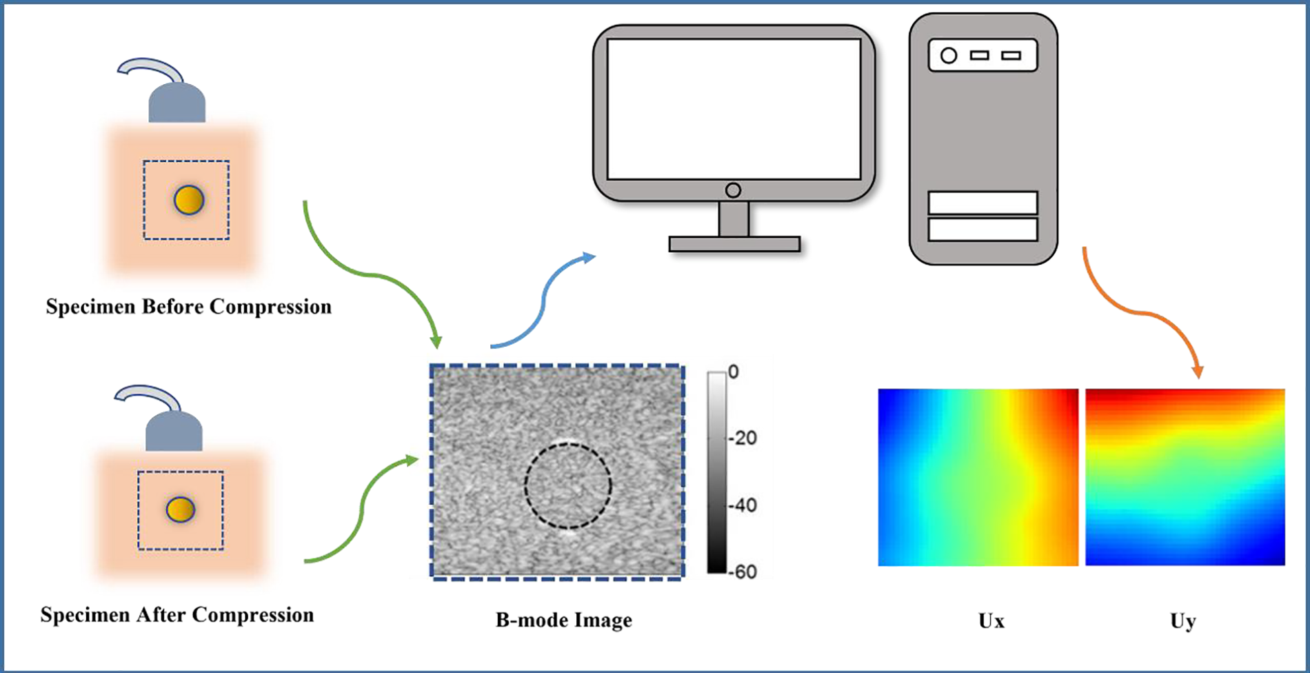
Figure 3: Illustration of experimental setup: Ultrasound and digital image correlation technics are used to obtain the measurement displacement fields

2.4 Assessment of the DL Model

To assess the performance of the DL models, we introduce two metrics: relative coverage ratio (RCR) [35] and the mean relative error (MRE) of shear modulus distribution. RCR is defined by:

RCR=Area of the detected inclusionsTarget area of the inclusions(7)

The area of the detected inclusion is defined as the entire area of the domain minus the area of the background. Inclusions are detected where the shear modulus value falls outside the range of the background, which has a shear modulus value ranging from 0–1.75 kPa.

MRE is defined by:

MRE=|μpred−μtargetμtarget|¯×100%(8)

where the bar over the variable means the average value of the relative error. μpred and μtarget are the predicted and target nodal shear moduli, respectively. Note that RCR should be close to one and MRE should be close to zero for a highly robust inverse scheme.

3  Results

In this section, we undertake a comparative analysis of the reconstructed outcomes derived from the proposed DL model in conjunction with the OP method, utilizing a selection of representative examples. Prior to delving into subsequent testing endeavors, a prerequisite step involves the evaluation of the convergence behavior exhibited by the DL model. As illustrated in Fig. 4, it becomes evident that both DL models, trained upon noise free and noisy datasets, respectively, attained a state of convergence satisfactorily following a span of 200 training epochs.

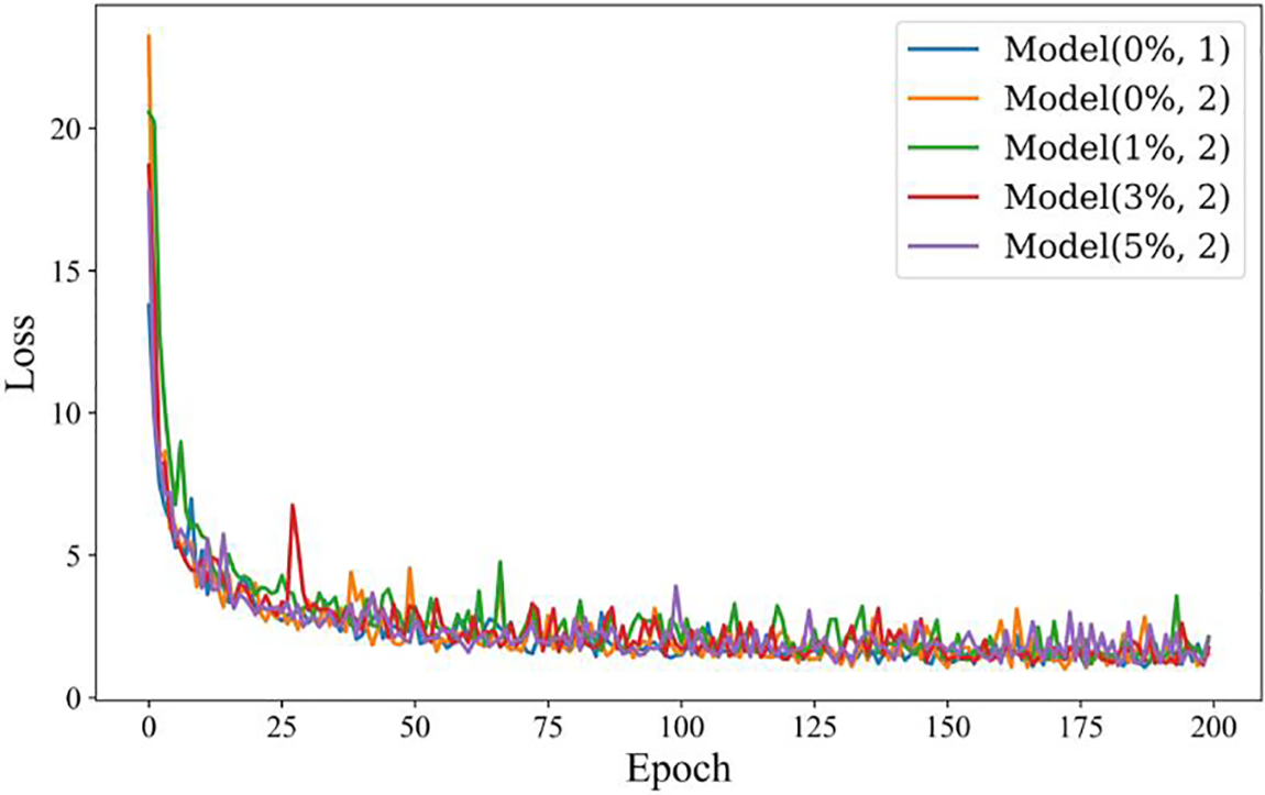
Figure 4: Plot of the loss function over the training epochs for the cGAN models we adopted, which includes models trained with both the noise-free and noisy datasets

3.1 Training Data Is Noisy Free

3.1.1 Training DL Model with Only One Inclusion

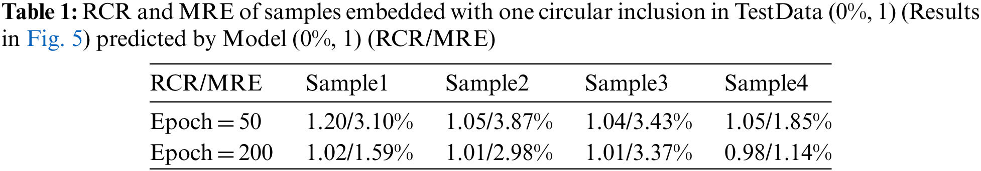
We first train the model with the noise-free simulated data (Model (0%, 1)). In the training datasets, we prescribe only one circular inclusion in the problem domain. The total number of the samples is 520 where 80% are used for training and 20% are used for testing. Fig. 5 presents four typical examples in the testing dataset with different epochs, the target shear moduli of the inclusion in Sample 1, Sample 2, Sample 3 and Sample 4 are 20, 16, 8 and 6 kPa, respectively. The target shear modulus of the background is 1 kPa in all four samples. The reconstructed results are very close to the target distribution. Table 1 shows that RCR approaches to 1 and MRE decreases with the increasing number of epochs. The excellent matching between the recovered and target shear modulus distributions demonstrate that the DL model is well trained.

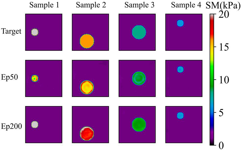
Figure 5: Predictions of noise-free one circular inclusion cases (TestData (0%, 1)) by Model (0%, 1). 1st row: Target shear modulus distribution; 2nd row: Predictions of shear modulus distribution after 50 training epochs; 3rd row: Predictions of shear modulus distribution after 200 training epochs

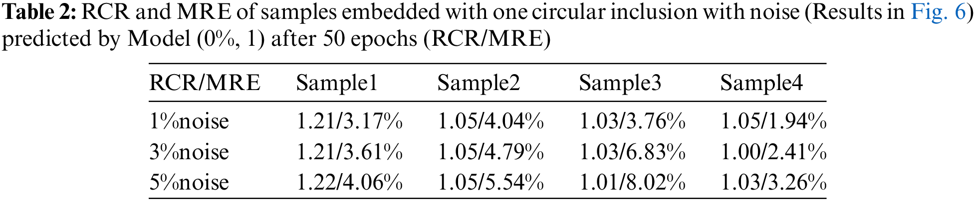
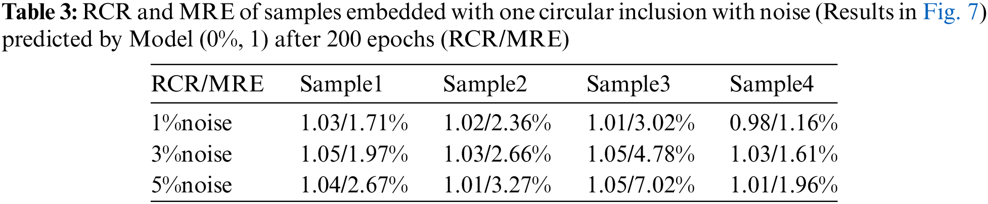
As shown in Fig. 6, we observe that the quality of the reconstructed shear modulus distribution becomes worse compared with Fig. 5. Moreover, with the increase of the noise level, the reconstructed results become worse. However, the shape and the shear modulus value of the inclusion are still well preserved. If we increase the number of epochs from 50 to 200 (See Fig. 7), we observe that the shear modulus value of the inclusion improves significantly as shown in Tables 2 and 3. Particularly, at 5% noise level, MRE decreases roughly from 5.22% (mean value) in Table 2 to 3.73% (mean value) in Table 3.

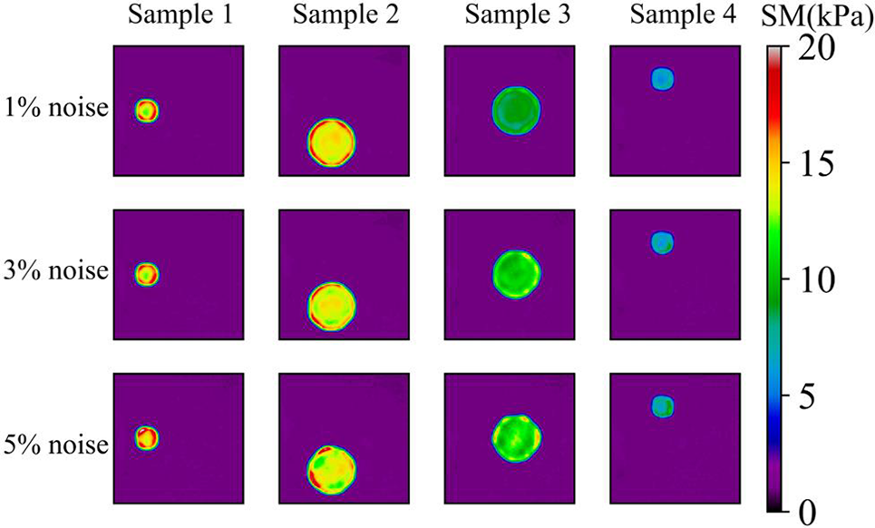
Figure 6: Predictions of noisy one circular inclusion test samples by Model (0%, 1) after 50 training epochs. 1st row: Shear modulus predictions of 1% noise (TestData (1%, 1)); 2nd row: Shear modulus predictions in the presence of 3% noise (TestData (3%, 1)); 3rd row: Shear modulus predictions in the presence of 5% noise (TestData (5%, 1))

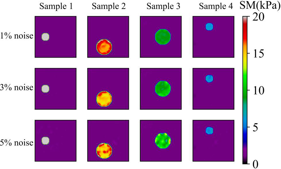
Figure 7: Predictions of noisy one circular inclusion test samples by Model (0%, 1) after 200 training epochs. 1st row: Shear modulus predictions of 1% noise (TestData (1%, 1)); 2nd row: Shear modulus predictions in the presence of 3% noise (TestData (3%, 1)); 3rd row: Shear modulus predictions in the presence of 5% noise (TestData (5%, 1))

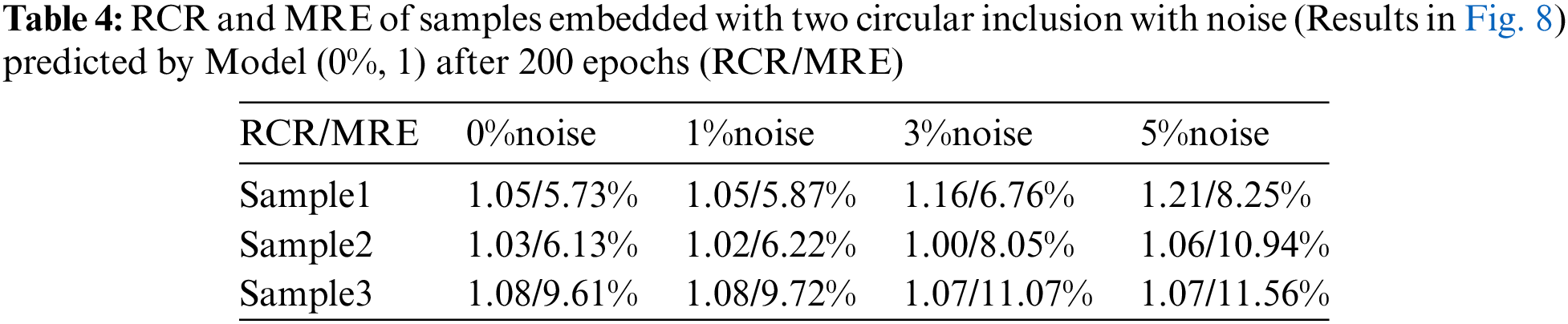
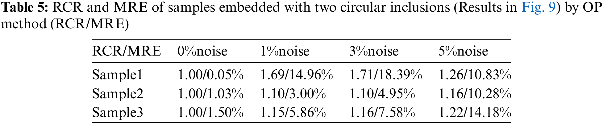
We also utilize the trained DL model to predict the cases with two inclusions. This is a challenging problem since we only used the cases with one inclusion to train the DL model. However, Fig. 8 demonstrates that the DL model trained with only one inclusion is capable of locating two inclusions with high accuracy. Even in the presence of 5% noise, the reconstructed results are of good quality. We also compare the reconstructed results by DL model with those obtained by the optimization-based method (see Fig. 9). One issue is that the background oscillates seriously for the optimization-based method. Moreover, the values of MRE are also larger for the optimization-based method compared Tables 4 and 5. Lastly, to preserve the shape of inclusions, the shear modulus values of the inclusions are far from the target.

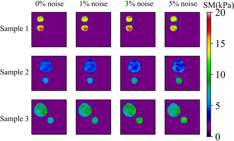
Figure 8: Predictions of two circular inclusion test samples by Model (0%, 1) after 200 training epochs. 1st column: Results in the case of noise-free (TestData (0%, 2)); 2nd column: Results in the presence of 1% noise (TestData (1%, 2)); 3rd column: Results in the presence of 3% noise (TestData (3%, 2)); 4th column: Results in the presence of 5% noise (TestData (5%, 2))

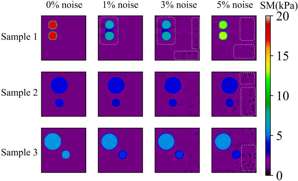
Figure 9: Results of two circular inclusion test sample shear modulus distribution by OP method. 1st column: Results of 0% noise (TestData (0%, 2)) ; 2nd column: Results of 1% noise (TestData (1%, 2)); 3rd column: Results of 3% noise (TestData (3%, 2)); 4th column: Results of 5% noise (TestData (5%, 2)). Regions with strong oscillation are marked with white dotted line

3.1.2 Training DL Model with Two Inclusions

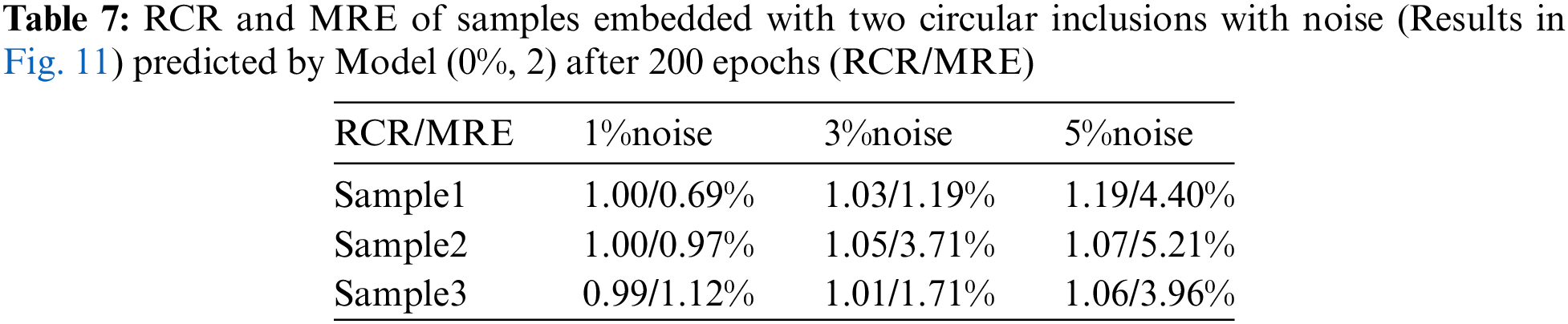
Next, we train another model with two inclusions embedded in the problem domain (Model (0%, 2)). In this case, we utilize 1040 samples where 80% is utilized for training and the rest 20% is utilized for testing. Fig. 10 shows the DL model is able to characterize the shear modulus distribution with high quality for the noise-free cases, the target shear modulus of the inclusions in Sample 1, Sample 2 and Sample 3 is 18, 4, 6 kPa, respectively. Table 6 shows that with higher epochs, the reconstructed results improve. If we add noise into the displacement fields in the testing samples (See Fig. 11), we observe that even with 5% noise in the displacement, the average error in MRE is 4.52% as shown in Table 7.

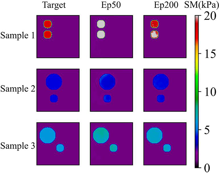
Figure 10: Predictions of two circular inclusion cases (TestData (0%, 2)) by Model (0%, 2). 1st column: Target shear modulus distribution; 2nd column: Predictions of shear modulus distribution after 50 training epochs; 3rd column: Predictions of shear modulus distribution after 200 training epochs

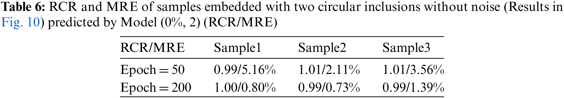
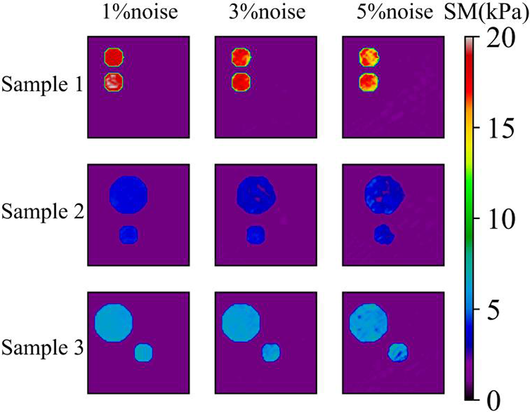
Figure 11: Predictions of two circular inclusion cases in the presence of noisy data by Model (0%, 2) after training 200 epochs. 1st column: Shear modulus distribution in the presence of 1% noise (TestData (1%, 2)); 2nd column: Shear modulus distribution in the presence of 3% noise (TestData (3%, 2)); 3rd column: Shear modulus distribution in the presence of 5% noise (TestData (5%, 2))

We also test the DL model with the experimental data as shown in Fig. 12. Since in the experimental setup and in vivo measurements [1], we are usually incapable of obtaining the applied loading, the shear modulus distribution is relatively mapped up to a multiplicative factor. We observe that the DL model with two inclusions is capable of yielding the decent reconstructed results. Particularly, the background appears very smooth compared with the optimization-based method.

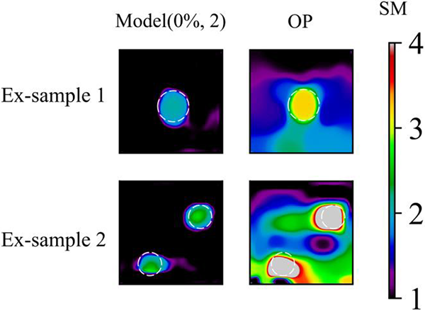
Figure 12: Comparison of experimental results by Model (0%, 2) and OP method. 1st column: Experimental shear modulus predictions by Model (0%, 2) after 200 training epochs; 2nd column: OP results of experimental sample. Target location of inclusions are marked with white dotted line

We also utilize the DL model to predict the target shear modulus distributions with different shapes of inclusions as shown in Fig. 13. Interestingly, the DL model performs well in recovering the shapes of the inclusions even we never trained the similar shapes of inclusions in the DL model (See Table 8). Besides, OP method generally outperforms the DL method in yielding the reconstructed results. Besides, to test the robustness of the DL model, we test the cases with more than two inclusions as shown in Fig. 14, we observe that the DL model is capable of reconstructing the shear modulus distribution well even with five inclusions embedded. However, in this particular case, the relative error between the predicted and target values of the shear modulus inclusions was found to be larger compared to previous cases.

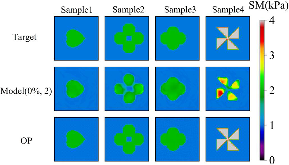
Figure 13: Comparison of cases with complicated shape of inclusion by Model (0%, 2) after 200 training epochs and OP method. 1st row: Target shear modulus distribution, the target shear modulus of the inclusions is 2, 2, 2, 4 kPa, respectively.; 2nd row: Predictions of shear modulus distribution by model trained with noise free dataset with two inclusions. 3rd row: Reconstructed results by OP method

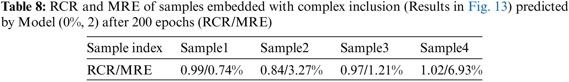
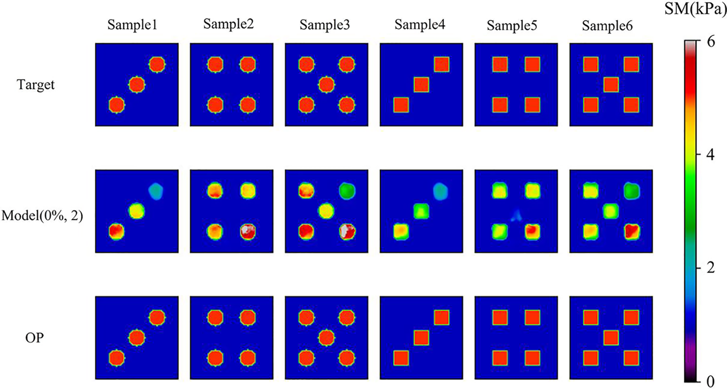
Figure 14: Comparison of cases with more than two inclusions by Model (0%, 2) after 200 training epochs and OP method. 1st row: Target shear modulus distributions for the multiple inclusion cases, the target shear modulus of the inclusions is all 5 kPa.; 2nd row: Predictions of shear modulus distributions by model trained with noise free dataset with two inclusions; 3rd row: Reconstructed shear modulus distributions by OP method

We conducted an empirical evaluation of the proposed methodology in two scenarios characterized by inhomogeneous inclusions, as illustrated in Fig. 15. In the first example, the target shear modulus distribution can be expressed by:

μ={1(x−0.5)2+(y−0.5)2>0.3521−50∗tanh[(x−0.5)2+(y−0.5)2−0.352](x−0.5)2+(y−0.5)2≤0.352(9)

Figure 15: (a) and (b) are target and the associated reconstructed shear modulus distributions for the case where the inclusion is inhomogeneous, respectively; (c) and (d) are target and the associated reconstructed shear modulus distributions for the case where one inclusion is emebedded into another inclusion, respectively

In this case, the shear modulus within the inclusion exhibits positional variance. As evidenced by the reconstruction outcome (depicted in Fig. 15b), the proposed DL methodology adeptly retains the spatial fluctuations inherent in the shear modulus of the inclusion. Nonetheless, it is noteworthy that the reconstruction quality is comparatively diminished with regard to the preceding examples, owing to the absence of pertinent training datasets encompassing inhomogeneous inclusions. In the second example (as portrayed in Fig. 15c), a stiffer, diminutive inclusion is enmeshed within a softer, encompassing inclusion. The proficiency of the DL model extends to the discernment of both inclusions. Nevertheless, the predictive accuracy of the local shear modulus values within select regions of the larger inclusion is notably compromised, primarily attributed to the dearth of training datasets germane to such compositional complexity (see Fig. 15d).

3.2 Training Data Is Noisy

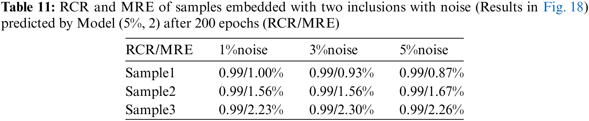
In this section, we will examine the influence of the noisy training data on the reconstructed shear modulus distribution. We firstly add 1% Gaussian noise into the training displacement datasets in the DL model with two inclusions as shown in Fig. 16. Compared with Fig. 11, the reconstructed results improve significantly in particular to the tested cases with 5% noise, the average MRE decreases from 4.52% to 1.90% (see Table 9). The similar observation has also been made by the DL models with training data in the presence of 3% and 5% noise as shown in Figs. 17 and 18. Compared with OP method (see Table 5), the DL method with noisy training data performs much better and the MRE values decrease significantly (see Tables 10 and 11).

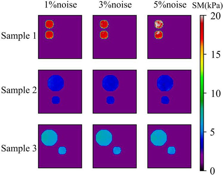
Figure 16: Predictions of cases with two circular inclusions by Model (1%, 2) after 200 training epochs. 1st column: Shear modulus predictions with 1% noise (TestData (1%, 2)); 2nd column: Shear modulus predictions with 3% noise (TestData (3%, 2)); 3rd column: Shear modulus predictions with 5% noise (TestData (5%, 2))

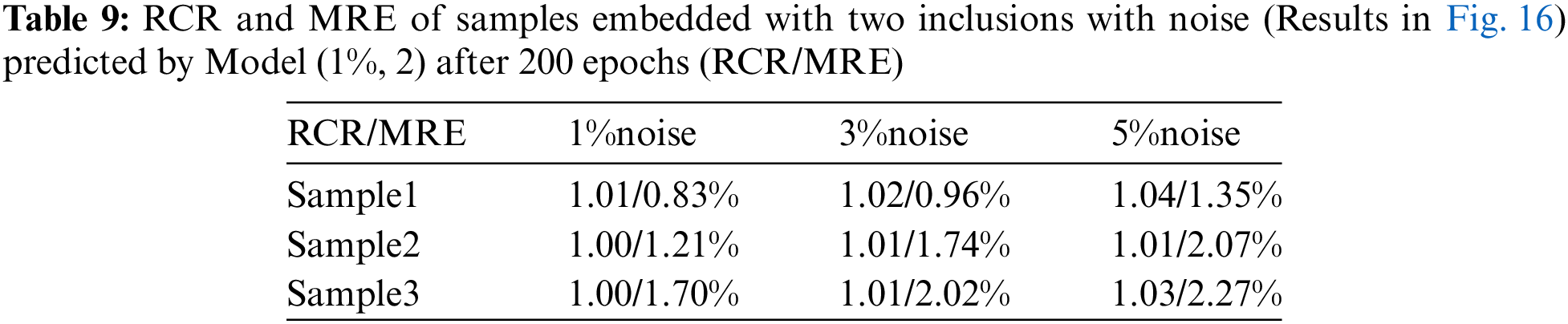
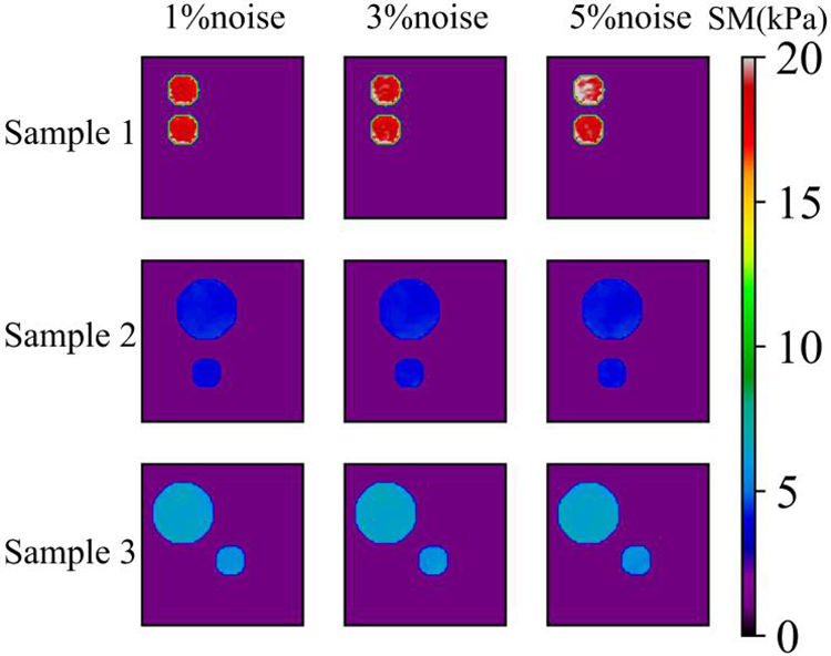
Figure 17: Predictions of cases with two circular inclusions by Model (3%, 2) after 200 training epochs.1st column: Predictions of shear modulus distributions in the presence of 1% noise (TestData (1%, 2)); 2nd column: Predictions of shear modulus distributions in the presence of 3% noise (TestData (3%, 2)); 3rd column: Predictions of shear modulus distributions in the presence of 5% noise (TestData (5%, 2))

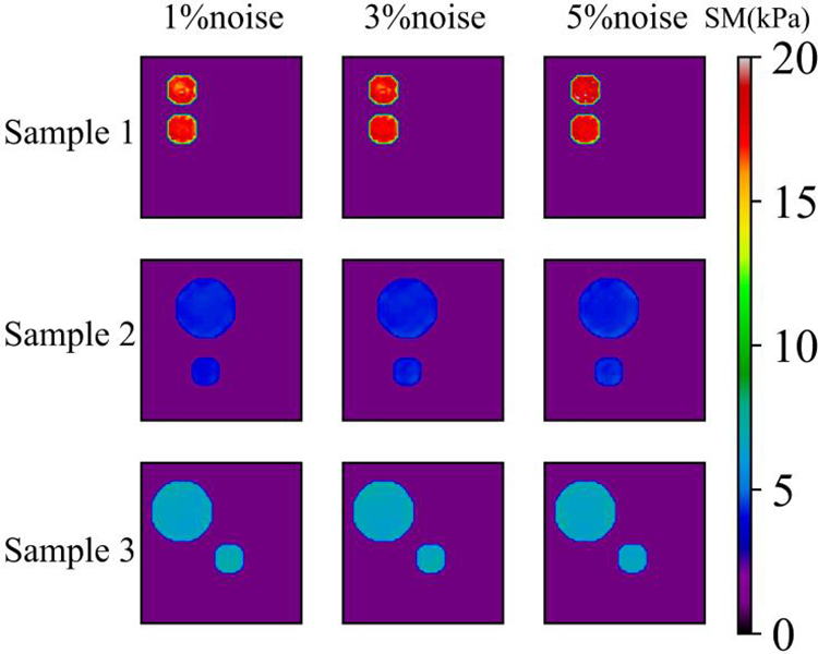
Figure 18: Predictions of noisy two circular inclusions test samples by Model (5%, 2) after 200 epochs. 1st column: Shear modulus predictions with 1% noise (TestData (1%, 2)); 2nd column: Shear modulus predictions with 3% noise (TestData (3%, 2)); 3rd column: Shear modulus predictions with 5% noise (TestData (5%, 2))

Further, the reconstructed results with experimental data improve as well compared with the results acquired by the associated DL model with noise free training data as shown in Fig. 19. Particularly, the shape of the recovered inclusion becomes more circular. The oscillation of the background also decreases significantly with DL model using noisy training data. Additionally, it seems that the DL model using training data with 3% noise yields the best reconstruction results.

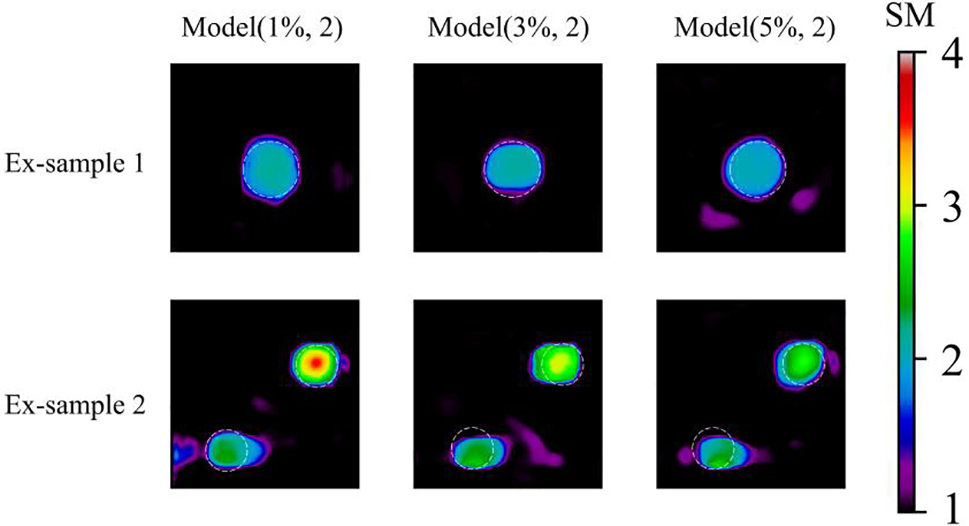
Figure 19: Predictions of the experimental sample after 200 training epochs. 1st column: Shear modulus predictions by Model (1%, 2); 2nd column: Shear modulus predictions by Model (3%, 2); 3rd column: Shear modulus predictions by Model (5%, 2). Target location of inclusions are marked with white dotted line

In addition, the performance of the entire test dataset is reported in Part A in the Supplementary Materials.

4  Discussion

In this paper, we propose to use the deep learning approach to solve the inverse problem in elasticity and characterize the nonhomogeneous shear modulus distribution utilizing both the simulated and experimental datasets. In the DL model, we merely utilized the simulated data for training in order to address the scarcity of clinical data. The simulated data originates from the finite element method, a rigorously established numerical technique renowned for its precision in simulating linear elasticity problem. This choice imparts a profound sense of dependability to our training dataset. Since the real datasets are noisy, we also added noise to the displacement fields in training and used exact shear modulus distribution as targets in order to reduce the influence of noise in the reconstructed results. Lastly, we used less than 1100 training samples whose embedded inclusions are merely circular to characterize the shear modulus distribution with complex geometries. It warrants attention that the introduction of noise into the simulated training dataset inherently introduces deviations from perfect alignment with real-world data, primarily attributed to the inherent uncertainties associated with boundary conditions and applied loadings. However, it is essential to emphasize that the ramifications of these disparities remain relatively modest when confronted with the complexities inherent in the resolution of inverse elasticity problems.

In elastography, how to minimize the influence of noise on the reconstructed elastic property distribution is highly challenging. We usually filter the noisy data to reduce the influence of noise [36–38]. However, DL approach provides an alternative way to address this issue. That is, we can inject noise to the simulated displacement fields in training. Since the DL model has already “learned” the noise in the training process, it is capable of reducing the influence of noise and recovering the elastic property distribution. The reconstructed results in this paper have shown great potential of this method in reconstructing the nonhomogeneous shear modulus distribution. Particularly, the reconstructed results by the proposed DL model are improved significantly compared to the results from the sophisticated OP methods. In the training datasets, we added the white Gaussian noise to the simulated displacements to mimic real-world data. However, studies have shown that the speckle tracking methods used can affect the noise and bias characteristics of the generated displacements [39]. Therefore, it is essential to conduct a comparative study to examine the impact of different speckle tracking methods on the final reconstructed results.

During the training process, we utilized less than 1100 samples, each containing no more than two circular inclusions. This is because the main objective of our work was to demonstrate the predictive capability of the DL model using synthetic datasets for experimental test samples. However, the DL model is able to solve the cases even with five inclusions with different shapes as shown in Figs. 13 and 14. Due to the fact that we solely trained the DL model using circular inclusions, the quality of the reconstructed results in this particular testing example is not as high as in other examples where only circular inclusions were present. In Fig. 14, we also observe that the inclusions displayed a clear trend of ‘hardening’ as they move further away from the compression surface. This phenomenon occurs as well in OP which has been fully discussed in [40,41].

Another critical issue in applying the DL model into clinical medicine is the scarcity of clinical data for model training. To address this issue, we used the simulated data generated by the finite element simulation as training data. As shown in Figs. 12 and 19, the models trained with simulated data are capable of reconstructing the nonhomogeneous shear modulus distribution with high quality. Thus, it is highly possible that we can utilize the simulated data as the main source of training data in cGAN-based elastography to supplement or even replace the clinical data. However, in order to assess the feasibility and reliability of the proposed method accurately, it is necessary to conduct future tests using real clinical datasets.

5  Conclusion

In this paper, we propose a DL model based on cGAN to improve the quality of the nonhomogeneous shear modulus distribution in elastography. In the training datasets, we utilize the simulated displacement data from the finite element simulation and the corresponding shear modulus distribution. To address the issue of noise in elastography, we add random noise to the simulated displacement fields. The reconstruction results demonstrate that DL models with both noisy and noise-free training data are capable of yielding reconstruction results with high quality. In particular, the DL model with noisy training datasets can improve the reconstruction results significantly compared to the optimization-based approach. Furthermore, we also test the proposed cGAN model on samples with more inclusions and more complex geometries than those in the training process. Collectively, the presented cGAN model demonstrates significant promise in harnessing the capabilities inherent in deep learning methodologies to enhance the caliber of reconstruction within the domain of elastography.

Acknowledgement: The authors acknowledge the support from the National Natural Science Foundation of China (12002075), National Key Research and Development Project (2021YFB3300601), Natural Science Foundation of Liaoning Province in China (2021-MS-128). We also thank Prof. Jianwen Luo from Tsinghua University for sharing the experimental datasets.

Funding Statement: National Natural Science Foundation of China (12002075), National Key Research and Development Project (2021YFB3300601), Natural Science Foundation of Liaoning Province in China (2021-MS-128).

Author Contributions: Yue Mei and Jianwei Deng wrote the main manuscript text. Jianwei Deng, Dongmei Zhao, Changjiang Xiao, Tianhang Wang wrote the code and ran all the examples. Yue Mei, Li Dong, Xuefeng Zhu came up with the idea. All authors reviewed the manuscript.

Availability of Data and Materials: Data available on request from the authors.

Conflicts of Interest: The authors declare that they have no conflicts of interest with the present studies.

References

1. Goenezen, S., Dord, J., Sink, Z., Barbone, P., Jiang, J. et al. (2012). Linear and nonlinear elastic modulus imaging: An application to breast cancer diagnosis. IEEE Transactions on Medical Imaging, 31(8), 1628–1637. [Google Scholar] [PubMed]

2. Sutphin, C., Olson, E., Motai, Y., Lee, S., Kim, J. et al. (2019). Elastographic tomosynthesis from X-ray strain imaging of breast cancer. IEEE Journal of Translational Engineering in Health and Medicine, 7, 1–12. [Google Scholar]

3. Ophir, J., Cespedes, I., Ponnekanti, H., Yazdi, Y., Li, X. (1991). Elastography: A quantitative method for imaging the elasticity of biological tissues. Ultrason Imaging, 13(2), 111–134. [Google Scholar] [PubMed]

4. Li, H., Peng, Y., Wang, Y., Hong, A., Zhou, X. et al. (2020). Elastography for the diagnosis of high-suspicion thyroid nodules based on the 2015 American thyroid association guidelines: A multicenter study. BMC Endocrine Disorders, 20(1), 43. [Google Scholar]

5. Gendin, D. I., Nayak, R., Wang, Y., Bayat, M., Fazzio, R. et al. (2021). Repeatability of linear and nonlinear elastic modulus maps from repeat scans in the breast. IEEE Transactions on Medical Imaging, 40(2), 748–757. [Google Scholar] [PubMed]

6. Liu, Z., Sun, Y., Deng, J., Zhao, D., Mei, Y. et al. (2020). A comparative study of direct and iterative inversion approaches to determine the spatial shear modulus distribution of elastic solids. International Journal of Applied Mechanics, 11(10), 1–17. [Google Scholar]

7. Luo, P., Mei, Y., Kotecha, M., Abbasszaderad, A., Rabke, S. et al. (2018). Characterization of the stiffness distribution in two and three dimensions using boundary deformations: A preliminary study. MRS Communications, 3(3), 893–902. [Google Scholar]

8. Lee, S., Kim, G., Han, B., Cho, M. (2011). Strain measurement from 3D micro-CT images of a breast-mimicking phantom. Computers in Biology and Medicine, 41(3), 123–130. [Google Scholar] [PubMed]

9. Dietrich, C., Barr, R., Farrokh, A., Dighe, M., Hocke, M. et al. (2017). Strain elastography-how to do it? Ultrasound International Open, 3(4), E137–E149. [Google Scholar] [PubMed]

10. Li, V., Liu, A., So, E., Ho, K., Yau, J. et al. (2019). Two-and three-dimensional myocardial strain imaging in the interrogation of sex differences in cardiac mechanics of long-term survivors of childhood cancers. International Journal of Cardiovascular Imaging, 35(6), 999–1007. [Google Scholar] [PubMed]

11. Mei, Y., Tajderi, M., Goenezen, S. (2017). Regularizing biomechanical maps for partially known material properties. International Journal of Applied Mechanics, 9(2), 1–23. [Google Scholar]

12. Smyl, D., Bossuyt, S., Liu, D. (2019). OpenQSEI: A MATLAB package for quasi static elasticity imaging. SoftwareX, 9, 73–76. [Google Scholar]

13. Barbone, P., Rivas, C., Harari, I., Albocher, U., Oberai, A. et al. (2010). Adjoint-weighted variational formulation for the direct solution of inverse problems of general linear elasticity with full interior data. International Journal for Numerical Methods in Engineering, 81(13), 1713–1736. [Google Scholar]

14. Ni, B., Gao, H. (2020). A deep learning approach to the inverse problem of modulus identification in elasticity. MRS Bulletin, 46(1), 19–25. [Google Scholar]

15. Mohammadi, N., Doyley, M., Cetin, M. (2021). Combining physics-based modeling and deep learning for ultrasound elastography. 2021 IEEE International Ultrasonics Symposium (IUS), pp. 1–4. Xi'an, China. [Google Scholar]

16. Mohammadi, N., Doyley, M., Cetin, M. (2021). Ultrasound elasticity imaging using physics-based models and learning-based plug-and-play priors. ICASSP 2021–2021 IEEE International Conference on Acoustics, Speech and Signal Processing (ICASSP), pp. 1165–1169. Toronto, Canada. [Google Scholar]

17. Chen, C., Gu, G. (2021). Learning hidden elasticity with deep neural networks. Proceedings of the National Academy of Sciences of the United States of America, 118(31), 1–8. [Google Scholar]

18. Patel, D., Tibrewala, R., Vega, A., Dong, L., Hugenberg, N. et al. (2019). Circumventing the solution of inverse problems in mechanics through deep learning: Application to elasticity imaging. Computer Methods in Applied Mechanics and Engineering, 353, 448–466. [Google Scholar]

19. Zhang, E., Yin, M., Karniadakis, G. E. (2020). Physics-informed neural networks for nonhomogeneous material identification in elasticity imaging. arXiv:2009.04525. [Google Scholar]

20. Tehrani, A. K., Rivaz, H. (2021). MPWC-Net++: Evolution of optical flow pyramidal convolutional neural network for ultrasound elastography. Medical Imaging 2021: Ultrasonic Imaging and Tomography, 11602, 14–23. [Google Scholar]

21. Tripura, T., Awasthi, A., Roy, S., Chakraborty, S. (2023). A wavelet neural operator based elastography for localization and quantification of tumors. Computer Methods and Programs in Biomedicine, 232, 107436. [Google Scholar] [PubMed]

22. Liu, Y., Chen, Y., Ding, B. (2022). Deep learning in frequency domain for inverse identification of nonhomogeneous material properties. Journal of the Mechanics and Physics of Solids, 168, 105043. [Google Scholar]

23. Reddy, J. (1993). An introduction to the finite element method. New York: Springer. [Google Scholar]

24. Rebsamen, M., Knecht, U., Reyes, M., Wiest, R., Meier, R. et al. (2019). Divide and conquer: Stratifying training data by tumor grade improves deep learning-based brain tumor segmentation. Frontiers in Neuroscience, 13, 1–13. [Google Scholar]

25. Rebsamen, M., Radojewski, P., McKinley, R., Reyes, M., Wiest, R. et al. (2022). A quantitative imaging biomarker supporting radiological assessment of hippocampal sclerosis derived from deep learning-based segmentation of T1w-MRI. Frontiers in Neurology, 13, 1–12. [Google Scholar]

26. Oberai, A., Gokhale, N., Feijoo, G. (2003). Solution of inverse problems in elasticity imaging using the adjoint method. Inverse Problems, 19(2), 297–313. [Google Scholar]

27. Mei, Y., Stover, B., Kazerooni, N., Srinivasa, A., Hajhashemkhani, M. et al. (2018). A comparative study of two constitutive models within an inverse approach to determine the spatial stiffness distribution in soft materials. International Journal of Mechanical Sciences, 140, 446–454. [Google Scholar]

28. Mirza, M., Osindero, S. (2014). Conditional generative adversarial nets. arXiv:1411.1784. [Google Scholar]

29. Isola, P., Zhu, J., Zhou, T., Efros, A. (2017). Image-to-image translation with conditional adversarial networks. Conference on Computer Vision and Pattern Recognition. https://doi.org/10.1109/cvpr.2017.632 [Google Scholar] [CrossRef]

30. Goodfellow, I., Pouget-Abadie, J., Mirza, M., Xu, B., Warde-Farley, D. et al. (2014). Generative adversarial nets. Proceedings of the 27th International Conference on Neural Information Processing Systems, vol. 2, pp. 2672–2680. [Google Scholar]

31. Ronneberger, O., Fischer, P., Brox, T. (2015). U-Net: Convolutional networks for biomedical image segmentation. Medical Image Computing and Computer Assisted Intervention Society, 9351, 234–241. [Google Scholar]

32. Wang, T., Liu, M., Zhu, J., Tao, A., Kautz, J. et al. (2018). High-resolution image synthesis and semantic manipulation with conditional GANs. Conference on Computer Vision and Pattern Recognition, Salt Lake City, UT, USA. [Google Scholar]

33. Pan, X., Liu, K., Bai, J., Luo, J. (2014). A Regularization-free elasticity reconstruction method for ultrasound elastography with freehand scan. Biomedical Engineering Online, 13(1), 1–17. [Google Scholar]

34. Pan, X., Gao, J., Tao, S., Liu, K., Bai, J. et al. (2014). A two-step optical flow method for strain estimation in elastography: Simulation and phantom study. Ultrasonics, 54(4), 990–996. [Google Scholar] [PubMed]

35. Liu, D., Du, J. (2021). Shape and topology optimization in electrical impedance tomography via moving morphable components method. Structural and Multidisciplinary Optimization, 64(2), 585–598. [Google Scholar]

36. Huang, T., Yang, G., Tang, G. (1979). A fast two-dimensional median filtering algorithm. IEEE Transactions on Acoustic, Speech and Signal Processing, 27(1), 13–18. [Google Scholar]

37. Varghese, T., Ophir, J. (1997). A theoretical framework for performance characterization of elastography: The strain filter. IEEE Transactions on Ultrasonics, Ferroelectrics, and Frequency Control, 44(1), 164–172. [Google Scholar] [PubMed]

38. Zhu, X., Chen, L., Liu, S., Fang, K., Wu, R. et al. (2021). An ultrasonic elastography method based on variable length of filter in strain computation. Sensing and Imaging, 22(1), 1–19. [Google Scholar]

39. Hild, F., Roux, S. (2012). Comparison of local and global approaches to digital image correlation. Experimental Mechanics, 52(9), 1503–1519. [Google Scholar]

40. Mei, Y., Goenezen, S., Doyle, B. J. et al. (2015). Spatially weighted objective function to solve the inverse problem in elasticity for the elastic property distribution. In: Computational biomechanics for medicine: New approaches and new applications, pp. 47–58. Cham: Springer. [Google Scholar]

41. Mei, Y., Kuznetsov, S., Goenezen, S. (2016). Reduced boundary sensitivity and improved contrast of the regularized inverse problem solution in elasticity. Journal of Applied Mechanics, 83(3), 1–10. [Google Scholar]

Supplementary Materials

The supplementary material consists of two parts. The first part outlines the overall performance of the trained DL models across the entire test dataset. The second part provides a brief introduction of the adopted OP method, including how we determined the regularization factor to mitigate the impact of measurement noise.

(A) Overall Performance of the entire test datasets

To better analyze the proposed DL method, we also summarize the overall performance of each trained DL model on the entire test sets by the boxplots of the MRE and RCR on each model. In each boxplot, the median value is shown in red dotted line. As shown in Fig. A1, MRE and RCR improves with the increasing of the total number of training epochs. Further, the median value of RCR approaches to 1 and the median value of MRE is only about 2% for the case of epoch 200. Fig. A2 reveals that with the increase of the noise level, MRE and RCR become worse due to the noise free training datasets. Comparing Figs. A3–A5, we observe that with the increasing of noise level of the test dataset, the results by the model trained by the noisy dataset performs much better than those trained with noise-free dataset. Both RCR and MRE of Model(0%, 1) are much worse than those from the noisy training model.

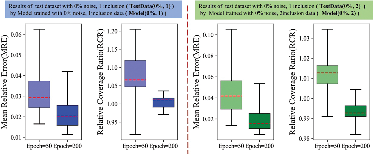
Figure A1: Boxplots of MRE and RCR by Model(0%, 1) and Model(0%, 2) in the noise-free training. From left to right: 1st: MRE boxplot of TestData(0%, 1) by Model(0%, 1); 2nd: RCR boxplot of TestData(0%, 1) by Model(0%, 1); 3rd: MRE boxplot of TestData(0%, 2) by Model(0%, 2); 4th: RCR boxplot of TestData(0%, 2) by Model(0%, 2). The blue boxes show the results of DL model trained with dataset embedded with one inclusion while the green boxes show the results of DL model trained with dataset embedded with two inclusions. Herein, the darker for the color means the model is trained with 200 epochs while the lighter color means the model is trained with 50 epochs

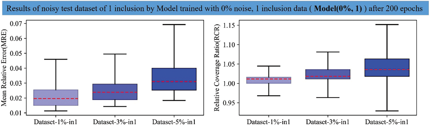
Figure A2: Boxplots of MRE and RCR by Model(0%, 1) on the TestData(1%, 1), TestData(3%, 1), TestData(5%, 1) after 200 training epochs. The left boxplot is the MRE results while the right one is the RCR results. From left to right in each boxplot: 1st: results on TestData(1%, 1); 2nd: results of TestData(3%, 1); 3rd: results of TestData(5%, 1). Blue color shows the results of DL model trained with noise-free dataset embedded with one inclusion and the darker the blue means the results on the test dataset with higher noise

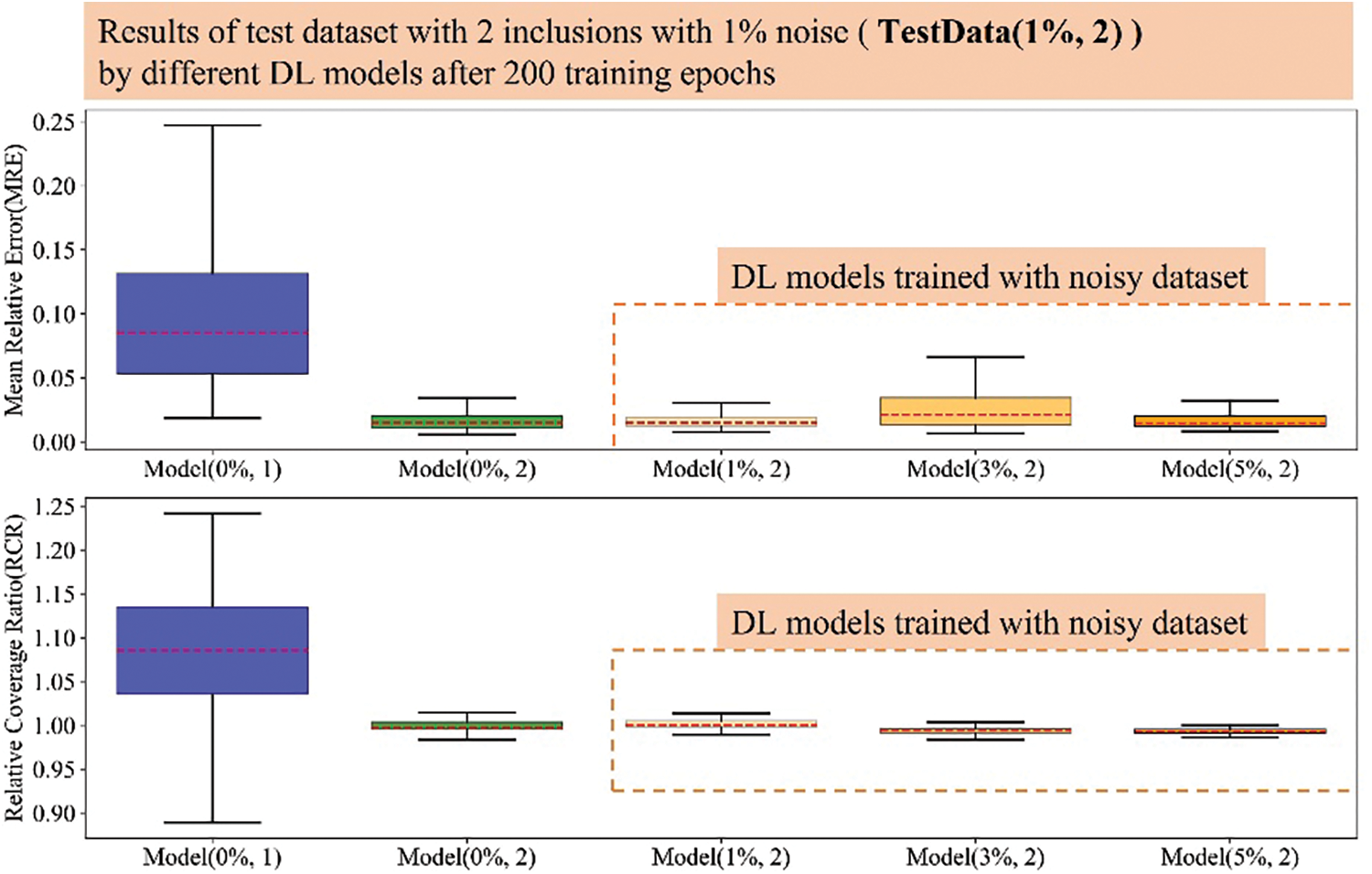
Figure A3: Boxplots of MRE and RCR by different models on TestData(1%, 2). The upper boxplot is the MRE results while the lower one is the RCR results. From left to right, 1st: Model(0%, 1); 2nd: Model(0%, 2); 3rd: Model(1%, 2); 4th: Model(3%, 2); 5th: Model(5%, 2). Herein, the blue boxes show the results of DL model trained with noise-free dataset embedded with one inclusion while the green box show the results of DL model trained with noise-free dataset embedded with two inclusions. The DL models trained with noisy dataset embedded with two inclusions is shown in orange color and the darker the orange color means the DL model trained with the training dataset with higher noise

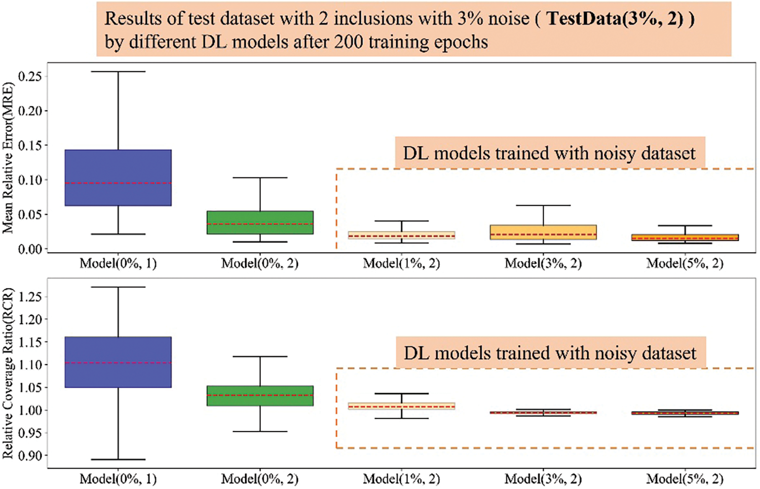
Figure A4: Boxplots of MRE and RCR by different models on Dataset-3%-in2. The upper boxplot is the MRE results while the lower one is the RCR results. From left to right, 1st: Model(0%, 1); 2nd: Model(0%, 2); 3rd: Model(1%, 2); 4th: Model(3%, 2); 5th: Model(5%, 2). Herein, the blue boxes show the results of DL model trained with noise-free dataset embedded with one inclusion while the green box show the results of DL model trained with noise-free dataset embedded with two inclusions. The DL models trained with noisy dataset embedded with two inclusions is shown in orange color and the darker the orange color means the DL model trained with the training dataset with higher noise

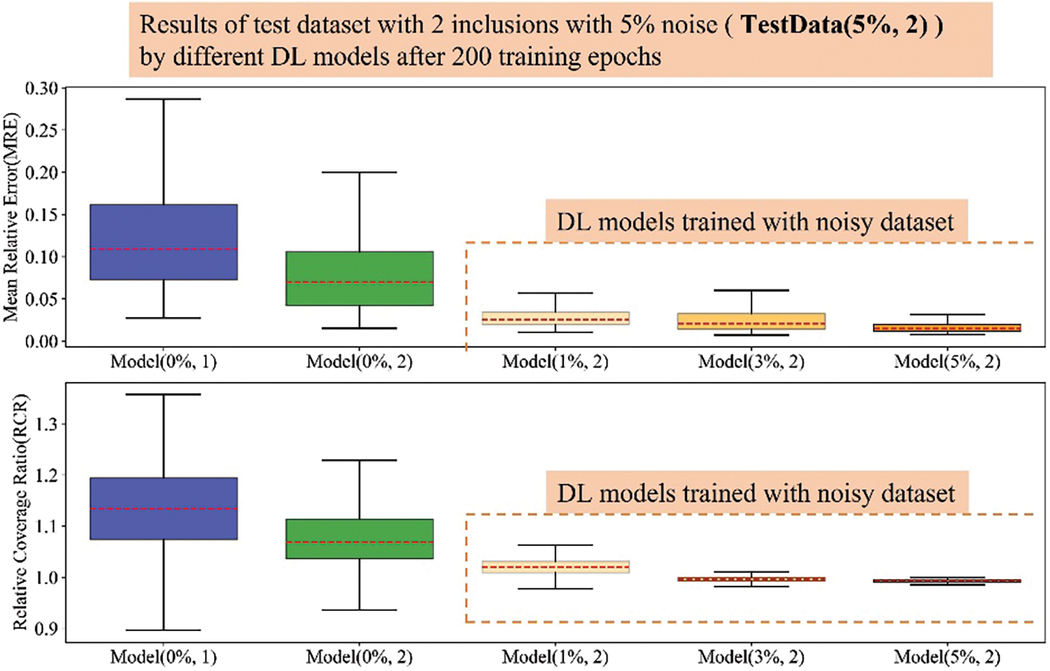
Figure A5: Boxplots of MRE and RCR by different models on Dataset-5%-in2. The upper boxplot is the MRE results while the lower one is the RCR results. From left to right, 1st: Model(0%, 1); 2nd: Model(0%, 2); 3rd: Model(1%, 2); 4th: Model(3%, 2); 5th: Model(5%, 2). Herein, the blue boxes show the results of DL model trained with noise-free dataset embedded with one inclusion while the green box show the results of DL model trained with noise-free dataset embedded with two inclusions. The DL models trained with noisy dataset embedded with two inclusions is shown in orange color and the darker the orange color means the DL model trained with the training dataset with higher noise

(B) The general procedure of the OP method

In this part, we make a brief introduction to the optimization-based inverse method. In OP method, the inverse problem is considered as a constrained optimization problem, where the forward process (in Eqs. (2)–(5)) is considered as the constrained condition. For reconstructing the nonhomogeneous distribution of shear modulus, the nodal shear modulus values are considered as optimization variables, which are updated until the objective function is minimized. The flowchart of the OP inverse method is shown in Fig. B1. The objective function is written as:

G∗=12∫Ω(u¯−umeas)2dΩ+Reg(μ)(B.1)

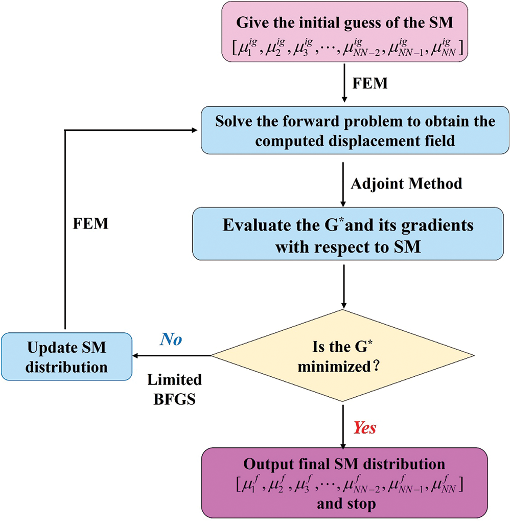
Figure B1: Flowchart of the OP method

The first term in Eq. (B.1) is the gap of the computed displacement field u¯ and the measured displacement field umeas. The second term is the total variational diminishing (TVD) regularization term, which is used to alleviate the influence of noise in the measurement displacement field:

Reg(μ)=12α∫Ω(∇μ)2+β2dΩ(B.2)

where α is the regularization factor, which controls the weight of the regularization term. The regularization factor can significantly impact the results of the reconstruction. To address this concern, we chose the regularization parameter based on the L-curve method, which has been shown to be effective in producing optimal reconstructed results. β is a small constant (herein is 0.01), which avoids singularity when calculating the gradient of the objective function.

In this paper, the limited Broyden–Fletcher–Goldfarb–Shanno (L-BFGS) method is used to solve constrained optimization problems. In each iteration step, the objective function and the gradient of the objective function for each optimization variable should be calculated, which is computationally expensive. The adjoint method is used to calculate the gradient of the objective function, which improves the calculation efficiency.