Spatial Distribution Feature Extraction Network for Open Set Recognition of Electromagnetic Signal

1  Introduction

Electromagnetic signal recognition (ESR) is a process of extracting features from a received signal and combining them with prior knowledge to identify the signal type or emitter. ESR, which includes modulation recognition and emitter recognition, plays an increasingly vital role in electronic reconnaissance. Traditional ESR relies on artificially designed extractors, and there are two methods: the likelihood-based approach [1–3] and the feature-based approach [4,5]. The former calculates the likelihood function of the signal, estimates the unknown parameters, and then compares it with the preset threshold to obtain the signal type. The latter method extracts features from the signal and compares them with theoretical values. However, the above methods need artificial design extractors to extract effective features from electromagnetic signals. This requires not only domain expertise and complex parameter tuning but also complex and massive calculations. In addition, traditional feature extractors are often sensitive to signal variations and interferences. Traditional methods will perform poorly in harsh working environments such as those containing noise or signal changes, which will cause misjudgment and recognition errors.

Due to the increasing complexity of the electromagnetic environment, deep learning-based methodologies have become the dominant approach. Traditional ESR methods have several limitations, including difficulties in extracting features and inadequate adaptability to complex modulation signals. The powerful capabilities of deep learning, including feature learning and pattern recognition, can help address these limitations [6,7]. In [8], a complex convolutional neural network was constructed for signal spectrum identification. A novel data-driven model based on Long Short-Term Memory (LSTM) was proposed in [9], which learns from training data without requiring expert features like higher-order cyclic moments. In [10], the authors designed an innovative network structure based on wavelet scattering convolution networks. In [11], authors used the adversarial losses of the feature layer and decision layer to generate adversarial examples with stronger attack performance. In addition, few-shot learning [12,13], semi-supervised learning [14–16], reinforcement learning [17] and lightweight models [18,19] for ESR were proposed, which were studied from the aspects of using a small amount of labeled training samples and reducing model complexity. However, they can only recognize the signal types seen in the training stage (known classes), which is called closed set recognition (CSR). In the case of signals that have never been seen before (unknown classes), CSR misclassifies them into known classes, which limits their application in the real world.

The real-world ESR task is usually limited by various objective factors, making it difficult to collect all signals required to train a classifier. Data quality and quantity play a key role in the development of deep learning models [20,21]. Samples of unknown classes often lack clear labels and class information, rendering existing ESR methods ineffective. Modern electromagnetic environments pose many security challenges, including radio spectrum competition, interference, and spoofing. Identification of unknown categories of samples is essential for signal safety. Due to the inability of traditional methods to identify and classify unknown samples effectively in modern electromagnetic environments, signal security is becoming increasingly critical. For example, in spectrum safety monitoring, unallocated frequencies are not allowed. In electromagnetic equipment supervision, only electromagnetic equipment included in the safety range can be operated. Other equipment is identified as non-allocated and cannot be operated. In the above cases, collecting all types of samples is not practical and can be solved using open set recognition (OSR). OSR acquires incomplete knowledge in training, and unknown classes can be submitted to the algorithm at testing [22]. Unlike CSR, OSR analyzes whether the sample type is known or not. OSR performs two tasks: classifying known class samples and rejecting unknown class samples. Specifically, OSR learns the features of each known class from the training set Strain containing only known classes. For the testing set Stest, which contains both known and unknown classes, OSR distinguishes known and unknown classes by comparing the sample features with the learned features of known classes, thereby rejecting unknown classes.

Traditional deep learning networks, such as convolutional neural networks (CNNs), use a Softmax classifier to address OSR. Softmax is a linear classifier that converts the output of multiple classifications into a probability distribution within the range [0,1] with a sum of 1. Because it divides the feature space based on the number of known classes, this classifier is insufficient for OSR tasks. Researchers explored two approaches to address this challenge. In the first approach, features derived from known class samples are used to predict unknown class samples, transforming the OSR problem into a CSR one. One notable method is the Openmax model [23] proposed by Bendale and Boult. This model assigns scores based on fitting a Weibull distribution and computes pseudo-activation vectors for unknown samples. Using Openmax, Prakhya et al. [24] explored open set text classification with promising results. Dang et al. [25,26] also incorporated extreme value theory into recognition methods to fit open set classifiers. To effectively model data distribution tails, these methods often require a solid understanding of probability statistics. However, they do not provide a principled approach to determining the tail size. Schlachter et al. [27] introduced a method that splits the given data into typical and atypical subsets using a closed set classifier. This enables the modeling of abnormal classes by leveraging atypical normal samples. However, determining the crucial hyperparameter split ratio for recognizing unknown class samples remains a challenge.

The second approach involves improving the learning methods or network frameworks of the models to enhance the consistency among samples from the same class and the distinctiveness between samples from different classes [28,29], thereby reducing the difficulty of recognizing unknown class samples. The more comprehensively known classes are acquired, the easier it is to reject unknown samples. Deep learning networks have a notable advantage as feature extractors since they can automatically extract features [30,31]. Hassen et al. [32] proposed learning a neural network-based representation for OSR that incentivizes projecting class samples around the class mean directly. Using Siamese networks, Wu et al. [33] proposed an identification method for open set emitters that relies on classification loss, reconstruction loss, and clustering loss. Yue et al. [34] improved the learned spectral-spatial features by reconstructing the spectral and spatial features. Yang et al. [35] combined prototype-based classifiers with deep CNN for robust pattern classification. However, most methods neglect the distribution features of samples in the feature space, namely inter-class distribution and intra-class distribution, despite the adoption of some clever loss functions. Nevertheless, these models still depend on the outputs of fully connected layers for their outputs.

Therefore, this paper proposes a spatial distribution feature extraction network (SDFEN). The network utilizes the spatial distribution information of samples as the network output for the classifier. To enhance the performance of the network, most methods [32,36,37] do not directly use cross-entropy loss to train the model. However, these loss functions either do not consider both inter-class and intra-class distributions or are not conducive to convergence. To train the model, SDFEN introduces a hybrid loss function that improves the form of the loss function. Almost all existing OSR methods adopt threshold-based classification schemes from the perspective of discriminative models [24,38,39]. A feature comparator compares depth features and thresholds to recognize unknowns.

The main contributions of this paper can be summarized as follows:

1)   A spatial distribution feature extraction network, i.e., SDFEN, is proposed for OSR of electromagnetic signals. SDFEN makes up for the lack of information between samples in traditional CNN. It uses the differences between samples as the main features extracted by the model, which is more suitable for recognition tasks.

2)   To model spatial distribution, a hybrid loss creates intra-class compactness and inter-class separation for feature learning. This method enhances intra-class consistency and inter-class differences, improving sample categorization.

3)   To distinguish between known and unknown classes, a feature comparator has been proposed which compares the spatial distribution feature with known class features. The feature comparator has been designed to effectively utilize spatial distribution information obtained from network outputs. This helps determine the boundaries between known and unknown classes in the feature space.

4)   Statistically significant improvement is achieved by the SDFEN in modulation recognition and emitter recognition, with up to 8.87% and 5.25% higher micro-F-measures respectively when compared to the state-of-the-art Openmax method.

The rest of this article is organized as follows: Section 2 introduces the framework of the spatial distribution feature extraction network in detail. This section will elaborate on the specific implementation process of the spatial distribution feature extractor, the Euclidean distance classifier, and the feature comparator. Section 3 describes the experimental settings in detail. The experiments will be conducted in both open and closed environments. The results show that the proposed method has significant advantages in modulation recognition and emitter recognition. Finally, Section 4 summarizes this paper and discusses our future work.

2  Spatial Distribution Feature Extraction Network

As shown in Fig. 1, SDFEN is composed of three main modules: the spatial distribution feature extractor (SDFE), the Euclidean distance classifier, and the feature comparator. The process involves mapping the original signal to a feature space using a spatial distribution feature extractor. Then, the Euclidean distance classifier predicts the type of signal, which belongs to a known class. The predicted label is then revised by comparing the spatial distribution feature with a threshold to obtain a corrected result. In addition, hybrid loss is used during training.

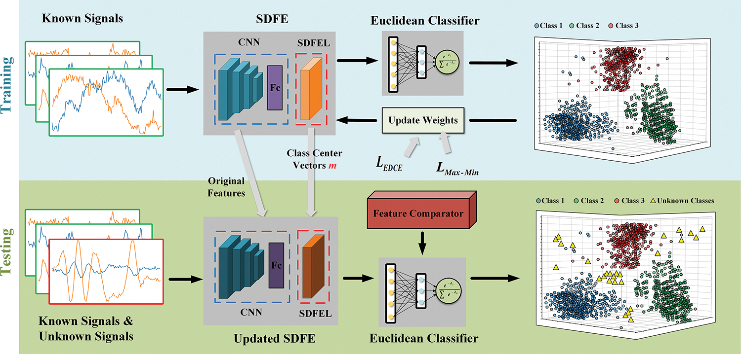
Figure 1: Framework of the spatial distribution feature extraction network (SDFEN)

2.1 Spatial Distribution Feature Extractor

SDFEN developed a spatial distribution feature extractor for extracting spatial distribution features from samples. By introducing specialized network structures and learning strategies, SDFEN enables the network to better extract and understand the spatial distribution relationship between samples, as well as to identify unknown samples. The spatial distribution feature extractor is improved based on CNN. Traditional CNN is usually composed of convolutional layers, pooling layers, and fully connected layers. As a result, convolutional layers and pooling layers are alternately applied, and then several fully connected layers are used to generate the final output. The convolutional layer uses the convolutional kernel to perform weighted summation on the input sample. CNNs can reduce training parameters by sharing weights across different local receptive fields. Traditional CNNs use the output after the full connection layer as the final feature and rely on the Softmax classifier for classification. As shown in Fig. 2, the spatial distribution feature extractor adds a spatial distribution feature extraction layer (SDFEL) to the traditional CNN. The spatial distribution feature extractor consists of two main components: a CNN and a spatial distribution feature extraction layer. SDFEL maps the original features obtained from the CNN to the depth features in the feature space. By introducing the class center vector, SDFEL captures spatial distribution information from the input signal. It calculates the distance between the feature vector and the class center vector to provide valuable similarity information for subsequent classifiers.

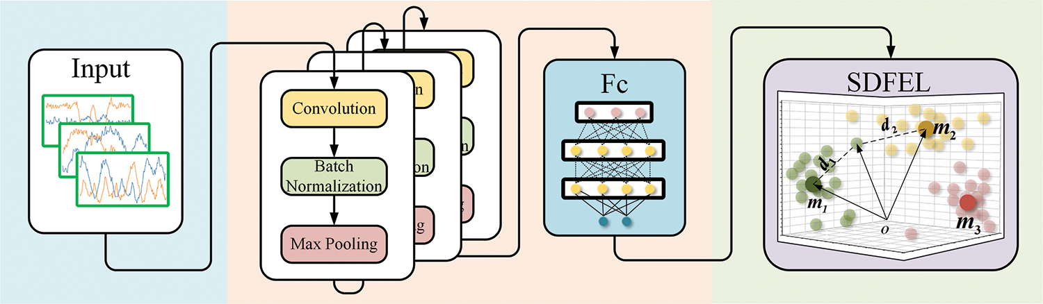
Figure 2: Framework of the spatial distribution feature extractor

CNN extracts the original features f(x,θ) from the input signal. Here, x and θ are the input data and CNN parameters, respectively. The SDFEL then takes the original features and processes them into depth features. To achieve this, the layer introduces a class center vector for each of the K known classes. The distance between the feature vector and the class center vectors in the feature space provides valuable similarity information for subsequent classifiers.

The SDFEL operates as follows for a recognition task with K known classes: 1) The original center vectors of the K known classes are randomly initialized, denoted as mi for class i. 2) The distances di between mi and f(x,θ) are calculated, which is given by:

di=d(f(x,θ),mi)=(f(x,θ)−mi)T(f(x,θ)−mi)(1)

Here, d(⋅) is the Euclidean distance function. The resulting spatial distribution feature, denoted as f′(x,θ,m), is given by:

f′(x,θ,m)=[d1,d2,⋯,dK](2)

where m=[m1,m2,⋯,mK] represents the class center matrix that will be updated during training using the spatial distribution feature extractor. 3) During the training process, the class center vector mi is updated with the CNN parameters θ.

SDFEL maps the original features obtained from the CNN to the depth features in the feature space. By incorporating the class center vectors into the feature extraction process, the spatial distribution feature extractor can effectively capture the spatial distribution information of the input signals. This information is then used to create a feature vector rich in similarity information. This feature vector can be effectively used by the subsequent classifier.

2.2 Euclidean Distance Classifier

The Euclidean distance classifier assesses the similarity between a signal and each known class based on the spatial distribution feature extracted by the spatial distribution feature extractor. The smaller the distance, the higher the similarity between the signal and the class. The probability that the signal sample x belongs to the class i is inversely proportional to the distance between f(x,θ) and mi, which can be expressed as:

pED(x∈mi|x)∝−d(f(x,θ),mi)(3)

The prediction label ypred can be expressed as:

ypred=argmax1≤i≤K⁡pED(x∈mi|x)=argmax(−f′(x,θ,m))(4)

Therefore, ypred can be obtained directly from the spatial distribution extractor f′(x,θ,m).

To ensure non-negativity and normalization of the probability, the expression of the Euclidean distance classifier is designed to be similar to the Softmax classifier. The probability that sample x belongs to class i is given by:

pED(x∈mi|x)=exp⁡(−d(f(x,θ),mi))∑k=1Kexp⁡(−d(f(x,θ),mk))(5)

Here, K is the number of known classes.

2.3 The Hybrid Loss Function

To improve OSR performance, signal samples of the same class are expected to be as close as possible in the feature space. In contrast, signal samples of different classes should be as far apart as possible. To achieve this, a hybrid loss function, denoted as LHybrid, is designed to optimize SDFEN parameters. LHybrid is composed of two parts: the cross-entropy loss based on Euclidean distance, denoted as LEDCE, and the Max-Min distance loss, called LMax-Min.

For a sample x with label y, LEDCE can be calculated as follows:

LEDCE=−log⁡pED(y|x)(6)

Essentially, optimizing LEDCE means reducing the distance between the original feature vector of x and the corresponding class y center vector. LEDCE is concerned with minimizing the distance between the feature vectors of samples with the same label and the corresponding class center vectors. This helps ensure that samples of the same class are close to each other in the feature space, which better captures their intrinsic similarities.

LMax-Min consists of the maximum intra-class distance dmax-intra and the minimum inter-class distance dmin-inter. The average distance between the class i samples and the class i center vector is defined as the class i intra-class distance. The maximum value of K intra-class distances is computed as dmax-intra, which is expressed as:

dmax-intra=max1≤i≤K⁡1Ni∑pd(f(xp(i),θ),mi)(7)

where xp(i) represents the p-th sample of class i, and Ni represents the number of samples in class i. The distance between the center vectors of two classes is calculated, and the minimum value is selected as dmin-inter, which is given by:

dmin-inter=min1≤i≤Ki+1≤j≤K⁡d(mi,mj)(8)

Therefore, following the principle of making the intra-class distance smaller and the inter-class distance larger, LMax-Min is designed as follows:

LMax-Min=dmax-intradmin-inter(9)

Finally, LHybrid can be expressed as:

LHybrid=LEDCE+λ⋅LMax-Min(10)

where λ is a hyperparameter in the range 0 to 1.

2.4 Feature Comparator

In this section, a feature comparator is proposed to identify unknown classes and adjust predicted results. The feature comparator works by comparing a threshold value τ and an outlier score scoreoutlier to determine the class of a given sample x. The corrected predicted result ypred′ for x is then obtained as follows:

ypred′={K+1,if scoreoutlier>τargmax(−f′(x,θ,m)),otherwise(11)

where K+1 represents the label of unknown classes. The outlier score scoreoutlier is defined as the distance between the sample x and its closest class in the feature space. Specifically, it is computed as follows:

scoreoutlier=min1≤i≤K⁡d(f(x,θ),mi)(12)

Obviously, the threshold is crucial for identifying unknown samples. As shown in Fig. 3, the larger the threshold, the more likely it is for some unknown samples to be wrongly classified as known ones. Conversely, setting a smaller threshold increases the risk of identifying known samples as unknown ones. Therefore, the threshold selection determines OSR effectiveness to some extent. To set τ, the training set is used to calculate the average intra-class distance davg-intra and the average inter-class distance davg-inter of the training samples. Similar to Eqs. (7) and (8), these values can be computed by:

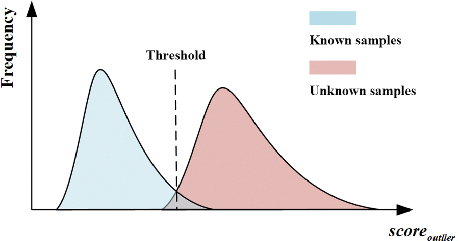
Figure 3: The influence of threshold on the recognition result

davg-intra=1N∑pd(f(xp,θ),mxp)(13)

davg-inter=1K2∑i,jd(mi,mj)(14)

o=davg-interdavg-intra(15)

The feature distribution measure o can be used to represent the distribution of signal samples in the feature space. To account for different learning degrees of different signals from various models, distinct feature distribution measures are set to correspond to distinct threshold rules, as follows:

τ={⌊davg-inter⌋2K+1,o>100davg-intra,o≤100(16)

3  Experiments and Analysis

3.1 Datasets Introduction

Two datasets of electromagnetic signals are used to evaluate modulation recognition and emitter recognition, respectively.

The experiments on modulation recognition will be carried out on the RADIOML 2016.10a dataset [40,41]. RADIOML 2016.10a dataset is a synthetic dataset generated with GNU Radio. It consists of 11 modulations, including 8PSK, AM-DSB, AM-SSB, BPSK, CPFSK, GFSK, 4PAM, 16QAM, 64QAM, QPSK, and WBFM. Each modulation is at varying signal-to-noise ratios (SNR), including −20, −18, −16, −14, −12, −10, −8, −6, −4, −2, 0, 2, 4, 6, 8, 10, 12, 14, 16, and 18 dB. Each SNR of each modulation has 1000 signals, for a total of 220000 signals. The complex valued IQ is processed as 128 × 2.

Emitter recognition experiments will be conducted on the ACARS dataset. ACARS is a digital data link system for short message transmission between aircraft and ground stations. It is designed to monitor aircraft running status and provide data support for maintenance personnel. The ACARS dataset in this paper is collected by an antenna system installed on the top of a high building in Jiaxing, Zhejiang Province, China. The dataset contains 16000 signals belonging to 20 different aircraft evenly. The complex valued IQ is processed as 4096 × 2.

3.2 Open Set Analysis

To approximate real-world scenarios, different levels of openness [42] have been simulated, which can be given by:

openness=1−2×|CTR||CTR|+|CTE|(17)

where CTR is the number of classes in training, and CTE is the number of classes in testing.

The OSR experiment uses evaluation indicators such as acceptance recognition rate (ARR), rejection rate (RR), and micro-F-measure [38] to measure the performance of the model. ARR represents the proportion of samples that should be accepted and correctly classified, while RR represents the proportion of samples that should be rejected. These indicators measure the recognition accuracy of the model for known and unknown classes, respectively. ARR and RR can be expressed as follows:

ARR = ∑i=1KTPi∑i=1K(TPi+FNi),RR = TPK+1TPK+1+FNK+1(18)

where TPi, TNi, FPi, and FNi denote the true positive, true negative, false positive, and false negative of class i, respectively. In addition, the micro-F-measure was used in the experiment to evaluate the overall recognition performance of the model. Micro-F-measure is defined as the adjusted average of micro-precision ratio Pmicro and micro-recall ratio Rmicro, which can be calculated by:

micro-F-measure = 2×Pmicro×RmicroPmicro+Rmicro(19)

Pmicro=∑i=1K+1TPi∑i=1K+1(TPi+FPi),Rmicro=∑i=1K+1TPi∑i=1K+1(TPi+FNi)(20)

3.3 Experiments on RADIOML 2016.10a Dataset

3.3.1 Experiment 1

In this particular experiment, the RADIOML 2016.10a dataset was used to simulate a closed set scene. To reduce the workload during training, certain SNRs were chosen, specifically −14, −12, −8, −4, −2, 0, 2, 4, 8, 12, and 14 dB. For each SNR, 75% of the signal samples were randomly selected as training samples, while the remaining were reserved for testing purposes.

In this study, a CNN was utilized as the primary feature extractor. Its structure is illustrated in Fig. 4a, where Conv denotes a convolutional layer module. Each convolutional layer module contains a convolutional layer, a maximum pooling layer, and a batch normalization layer. The original features extracted from the CNN are fed into the spatial distribution feature extraction layer, followed by the hybrid loss function for network training. The batch size of the CNN was set to 100, and the number of iterations was set to 500. The optimizer used was stochastic gradient descent (SGD), with an initial learning rate of 0.05. The hyperparameter of (10) was set to 0.3. Four approaches were evaluated. The first approach (Softmax) used Softmax as the classifier and applied cross-entropy loss while training. The second approach (II-Loss+CE), as described in [32], used both II-Loss and cross-entropy loss as the training objective. The third approach (GCPL) incorporates prototypes into the model and adds prototype losses to train the network [36]. The fourth approach (Hybrid) used LHybrid.

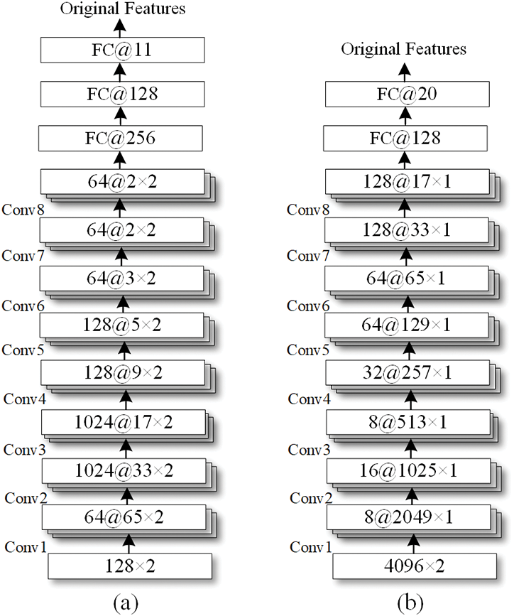
Figure 4: The structures of the CNN for modulation recognition and emitter recognition

To enable a comparative analysis of the recognition accuracy of the four method sets, we present the confusion matrices for each method in Fig. 5. Additionally, we illustrate the recognition accuracy of the four methods under different SNRs in Fig. 6. The closed set recognition accuracy of the four methods are 61.99%, 62.80%, 63.01%, and 64.84%, respectively. As depicted in Fig. 5, Softmax and II-Loss+CE show weak recognition abilities for 16QAM and WBFM signals. GCPL performs better than Softmax and II-Loss+CE, while Hybrid outperforms the others in recognizing these two types of signals. Moreover, Hybrid performs better in recognizing BPSK, GFSK, and 4PAM signals. As demonstrated in Fig. 6, recognition accuracy is positively correlated with SNR. Overall, the four methods exhibit higher recognition performance at SNRs of 0, 2, 4, 6, 8, 10, 12, and 14 dB. In general, Hybrid has superior advantages over the other methods.

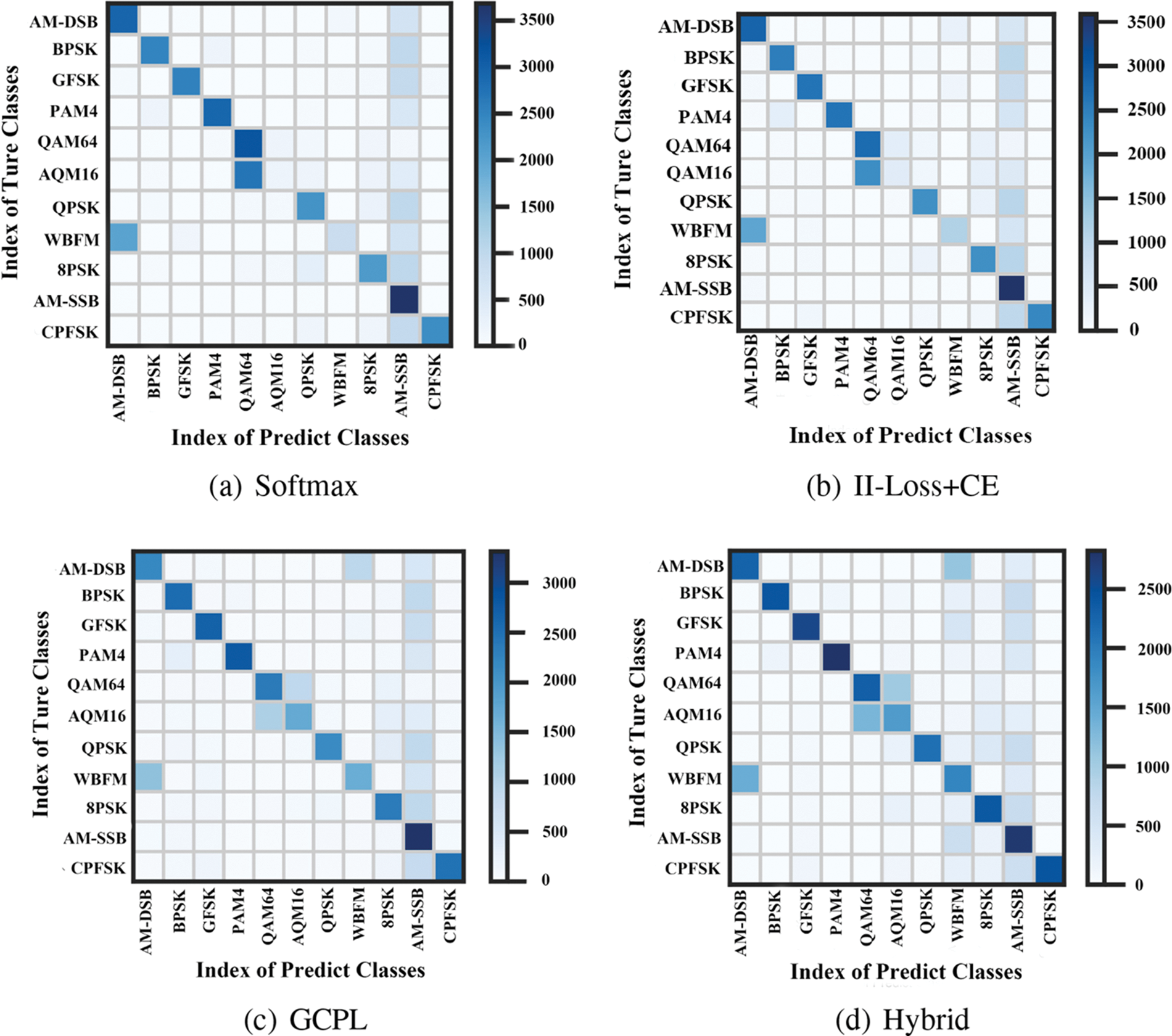
Figure 5: Confusion matrices of four methods for modulation recognition

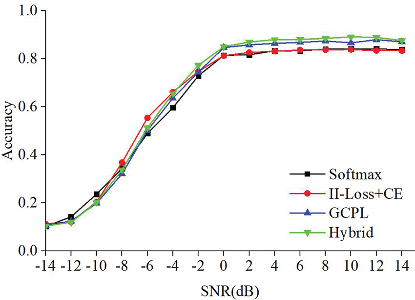
Figure 6: Comparison of modulation recognition accuracy with SNR

To validate the effectiveness of the proposed method in modeling distribution features, the distributions of signal samples under four methods in the feature space are illustrated in Fig. 7. The performance is demonstrated using BPSK, GFSK, PAM4, QPSK, 8PSK, and CPFSK with an SNR of 10 dB to avoid being influenced by poorly recognized signal types. The results show that II-Loss+CE, GCPL, and Hybrid, which utilize distance features as the loss function, exhibit stronger discriminative power in spatial distributions than Softmax, which uses traditional cross-entropy loss. In general, the proposed method demonstrates more compact intra-class distributions and more distant inter-class distributions.

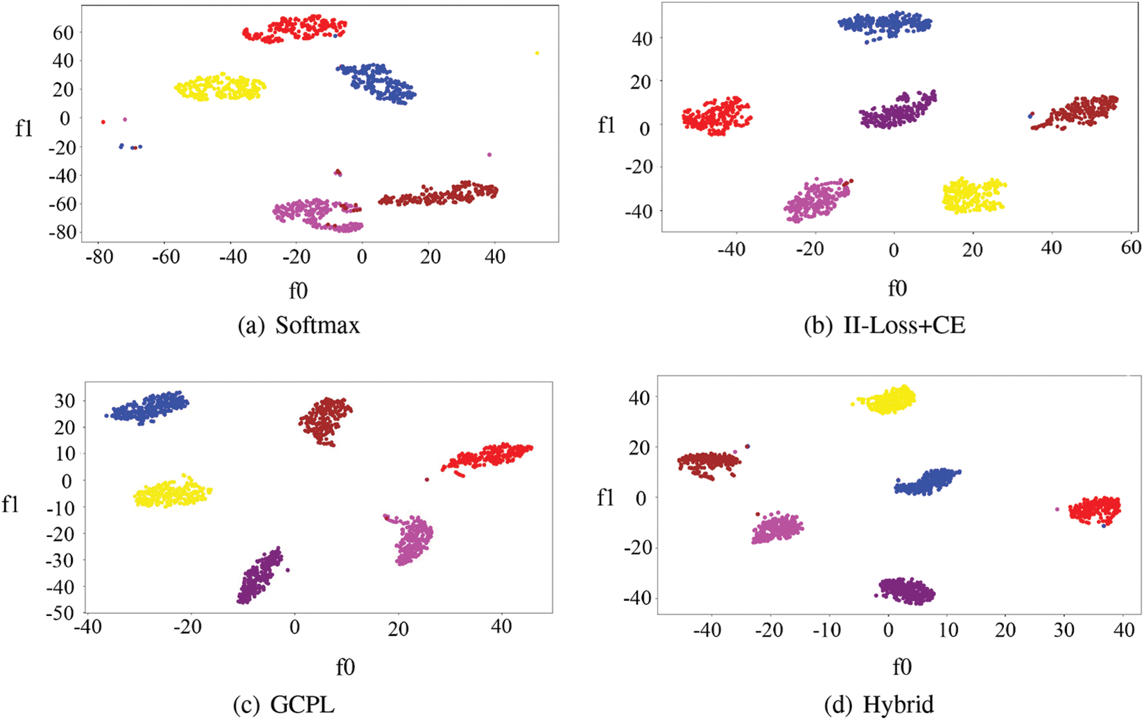
Figure 7: Spatial distribution feature of four modulation recognition methods

Out of the four methods mentioned, Softmax directly relies on the output of the original features from the fully connected layer for classification. This is without considering the distribution of samples in the feature space. On the other hand, II-Loss, GCPL, and Hybrid take into account the distribution of samples in the feature space. However, GCPL does not consider inter-class distances while II-Loss includes intra-class distances but its loss function is not conducive to model convergence. Hybrid, unlike the other three methods, considers both inter-class and intra-class distances with a loss function designed in the form of a ratio to make the model easier to train. This method exhibits smaller intra-class distances and larger inter-class distances, which benefit the recognition and OSR task. By increasing the inter-class distance and decreasing the intra-class distance, more space in the feature space can be left for unknown samples and the difference between known and unknown classes can be more pronounced during classification.

3.3.2 Experiment 2

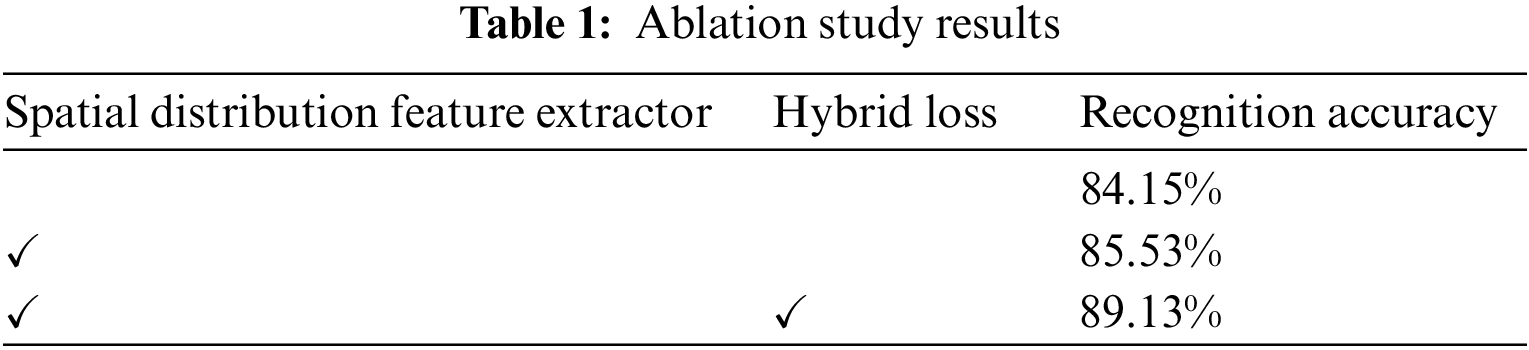
An ablation study was carried out to verify the effectiveness of the spatial distribution feature extractor and the hybrid loss function in the proposed method. RADIOML 2016.10a dataset was used and signal samples with 10 dB SNR were chosen. Seventy-five percent of the signal samples were randomly chosen as training samples, and the rest were selected for testing. The specific structure and parameter settings of the model used in the experiments were the same as Experiment 1 in Section 3.3.1. The experimental results are shown in Table 1. As the results show, the deep learning model with the feature extractor has significantly higher recognition accuracy than the model without the feature extractor. In addition, training the model with the hybrid loss function resulted in better recognition performance.

3.3.3 Experiment 3

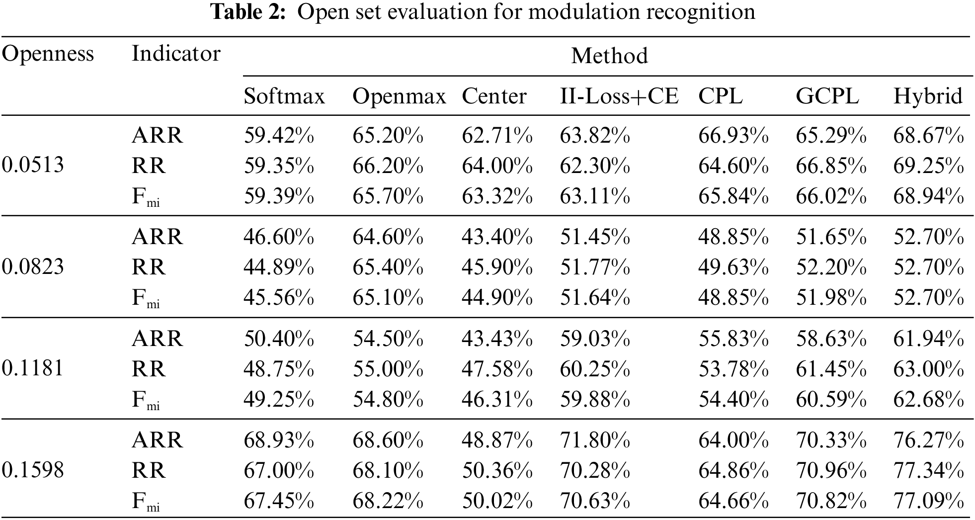
In this experiment, the open set scene was simulated on the RADIOML 2016.10a dataset and signal samples with an SNR of 10 dB were chosen. The number of unknown classes was set to 2, 3, 4, and 5, respectively, and the remaining classes were known. Similarly, 75% of the signal samples of known classes were randomly selected as training samples, and the rest were used for testing. Therefore, the corresponding openness is 0.0513, 0.0823, 0.1181 and 0.1598.

Seven different methods were compared, excluding the four methods described in Section 3.3.1, Softmax, II-Loss+CE, GCPL, and Hybrid. Additionally, three more methods were added: Center [37], which utilized Center Loss for model training; CPL [36], which uses convolutional prototype learning to learn features; and Openmax, the state-of-the-art OSR method. In Table 2, the ARR, RR, and micro-F-measure of these methods in different openness is illustrated. The micro-F-measure in the table is abbreviated as Fmi. It is evident that in the open set scene, Hybrid performed overall better than the other methods in the classification of known classes and rejection of unknown classes. This is at the same openness level. When the openness is 0.1598, the proposed Hybrid method outperforms the state-of-the-art Openmax method by 8.87% in terms of the micro-F-measure. At the same time, the ARR is 7.76% higher and the RR is 9.24% higher. Combined with the CSR results in Section 3.3.1, it can be observed that methods with higher accuracy in CSR also exhibit better performance in OSR. Furthermore, there is significant variation in the recognition performance of the same method at different openness levels. However, as openness increases, recognition performance does not decrease. This can be understood by considering the inherent differences in class recognition performance due to variations among known classes, as demonstrated in Fig. 5. Therefore, an increase in the number of known classes does not necessarily mean open set recognition becomes easier.

3.4 Experiments on ACARS Dataset

3.4.1 Experiment 1

In this experiment, the closed set scene was simulated on the Acars dataset. Seventy-five percent of the signal samples were randomly selected as training samples and the rest for testing. Fig. 4b shows the CNN structure for emitter recognition. The batch size was set to 100, the number of iterations was set to 500, SGD was selected as the optimizer, the initial learning rate was adjusted to 0.05, and the hyperparameter of (10) was set to 0.3. Similarly, Softmax, II-Loss, and Hybrid were evaluated.

The closed set recognition accuracy of the four methods are 98.68%, 98.20%, 98.45%, and 99.18%, respectively. Similarly, the distributions of samples in the feature space under the four methods are shown in Fig. 8. Compared with Softmax, GCPL, and II-Loss+CE, the proposed method has a larger average inter-class distance and a smaller average intra-class distance. Hybrid also achieves closed set recognition accuracy.

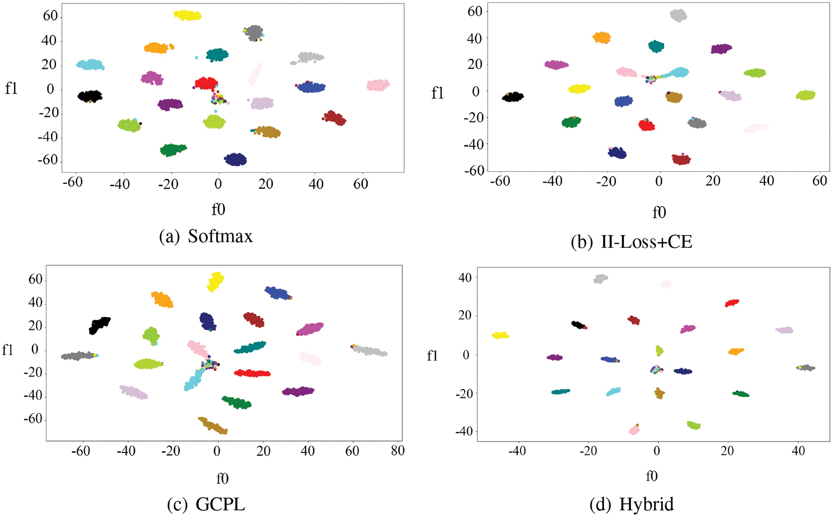
Figure 8: Spatial distribution feature of four emitter recognition methods

3.4.2 Experiment 2

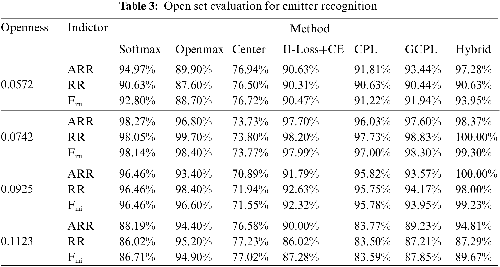
In this experiment, the open set scene was simulated on the ACARS dataset and the number of unknown classes was set to 4, 5, 6, and 7, respectively. Then the corresponding openness is 0.0572, 0.0742, 0.0925, and 0.1124. Similarly, 75% of the signal samples of known classes were randomly selected as training samples, and the rest were used for testing.

Similar to Section 3.3.3, seven methods are evaluated. The results are shown in Table 3. Obviously, in the open set scene, Hybrid performs overall better than the others in the classification of known classes and rejection of unknown classes. When the openness is 0.0572, the proposed method Hybrid outperforms the state-of-the-art Openmax method by 5.25% in terms of micro-F-measure. At the same time, the ARR is 7.38% higher and the RR is 3.03% higher. The Hybrid extracts spatial distribution features for classification, and direct feedback on the similarity between samples of the same class and the difference between samples of different classes into the model for training, which enables the model to directly model the distribution of samples in the feature space, so that similar samples are closer to each other and different samples are farther away. Therefore, unknown class samples can have a larger activity space. Let unknowns not overlap with known class samples. Combined with the experimental results in Section 3.4.1, it can also be inferred that methods that perform better on CSR have a positive effect on OSR.

It is true that the Hybrid has some advantages in the field of OSR. However, OSR experimental results show that the proposed method is sensitive to openness like most other methods. In essence, the model itself recognizes the differences between various types of samples, which affects recognition effects under different openness. Further research is needed on OSR which is more robust under different openness.

4  Conclusion

To address the recognition problem of electromagnetic signals in the open set environment and cope with the increasingly complex electromagnetic environment, this paper proposes a novel SDFEN. SDFEN introduces a dedicated network structure and learning strategy to better extract and understand spatial distribution relationships between samples. This supports the recognition of unknown class samples. The SDFEL in SDFEN is specifically designed to make up for the lack of information between samples in traditional CNN. It utilizes the differences between samples as the main features extracted by the model, which is more suitable for recognition tasks. To enhance intra-class consistency and inter-class differences, SDFEN designs a loss function that brings samples of the same class closer together in the feature space while increasing the distance between samples of different classes. This feature learning approach helps differentiate between different class samples and provides stronger discriminative capabilities. Additionally, SFDEN introduces a feature comparator to compare the features of samples with the learned features of known class samples. This distinguishes between known and unknown class samples. By comparing the distances or similarities between features, SFDEN can determine whether a sample belongs to a known class. The proposed method is validated in modulation recognition and emitter recognition tasks. The distribution plots of samples in the feature space under Softmax, GCPL, II-Loss+CE, and Hybrid provide evidence that the proposed method enhances the intra-class compactness of similar samples while increasing the separation between different class samples. Compared with other methods in simulated open set scenarios, the proposed method shows better overall performance. Specifically, in comparison to the state-of-the-art Openmax method, the proposed method achieves up to 8.87% and 5.25% higher micro-F-measures respectively. However, the experimental results also indicate that the proposed method is sensitive to openness, suggesting the need for further exploration of more robust OSR methods.

Acknowledgement: The authors wish to express their appreciation to the reviewers for their helpful suggestions which greatly improved the presentation of this paper.

Funding Statement: The authors received no specific funding for this study.

Author Contributions: The authors confirm contribution to the paper as follows: study conception and design: Hui Zhang, Huaji Zhou; data collection: Li Wang; analysis and interpretation of results: Li Wang, Feng Zhou; draft manuscript preparation: Hui Zhang, Feng Zhou. All authors reviewed the results and approved the final version of the manuscript.

Availability of Data and Materials: This paper uses two datasets. The first is the RADIOML 2016.10a dataset, which can be found at https://www.deepsig.ai/datasets. The second is the real-world ACARS dataset, which is collected by the antenna system installed on the top of a high building in Jiaxing, Zhejiang Province, China. Since this dataset is currently being used in many other studies, it is confidential.

Conflicts of Interest: The authors declare that they have no conflicts of interest to report regarding the present study.

References

1. Zhou, H. J., Bai, J., Wang, Y. R., Jiao, L. C., Zheng, S. L. et al. (2022). Few-shot electromagnetic signal classification: A data union augmentation method. Chinese Journal of Aeronautics, 35(9), 49–57. [Google Scholar]

2. Chavali, V. G., Da Silva, C. R. (2011). Maximum-likelihood classification of digital amplitude-phase modulated signals in flat fading non-gaussian channels. IEEE Transactions on Communications, 59(8), 2051–2056. [Google Scholar]

3. Hameed, F., Dobre, O. A., Popescu, D. C. (2009). On the likelihood-based approach to modulation classification. IEEE Transactions on Wireless Communications, 8(12), 5884–5892. [Google Scholar]

4. Wu, H. C., Saquib, M., Yun, Z. (2008). Novel automatic modulation classification using cumulant features for communications via multipath channels. IEEE Transactions on Communications, 7(8), 3098–3105. [Google Scholar]

5. Dobre, O. A., Abdi, A., Bar-Ness, Y., Su, W. (2007). Survey of automatic modulation classification techniques: Classical approaches and new trends. IET Communications, 1(2), 137–156. [Google Scholar]

6. Liu, M., Zhang, H., Liu, Z., Zhao, N. (2023). Attacking spectrum sensing with adversarial deep learning in cognitive radio-enabled internet of things. IEEE Transactions on Reliability, 72(2), 431–444. [Google Scholar]

7. Liu, M., Liu, C., Chen, Y., Yan, Z., Zhao, N. (2023). Radio frequency fingerprint collaborative intelligent blind identification for green radios. IEEE Transactions on Green Communications and Networking, 7(2), 940–949. [Google Scholar]

8. Kumar, Y., Sheoran, M., Jajoo, G., Yadav, S. K. (2020). Automatic modulation classification based on constellation density using deep learning. IEEE Communications Letters, 24(6), 1275–1278. [Google Scholar]

9. Rajendran, S., Meert, W., Giustiniano, D., Lenders, V., Pollin, S. (2018). Deep learning models for wireless signal classification with distributed low-cost spectrum sensors. IEEE Transactions on Cognitive Communications and Networking, 4(3), 433–445. [Google Scholar]

10. Zhou, H., Jiao, L., Zheng, S., Chen, S., Yang, L. et al. (2019). Weight-variable scattering convolution networks and its application in electromagnetic signal classification. IEEE Access, 7, 175889–175896. [Google Scholar]

11. Liu, M., Zhang, Z., Chen, Y., Ge, J., Zhao, N. (2023). Adversarial attack and defense on deep learning for air transportation communication jamming. IEEE Transactions on Intelligent Transportation Systems, 1–14. https://doi.org/10.1109/TITS.2023.3262347 [Google Scholar] [CrossRef]

12. Che, J., Wang, L., Bai, X., Liu, C., Zhou, F. (2022). Spatial-temporal hybrid feature extraction network for few-shot automatic modulation classification. IEEE Transactions on Vehicular Technology, 71(12), 13387–13392. [Google Scholar]

13. Dong, Y., Jiang, X., Zhou, H., Lin, Y., Shi, Q. (2021). SR2CNN: Zero-shot learning for signal recognition. IEEE Transactions on Signal Processing, 69, 2316–2329. [Google Scholar]

14. Dong, Y., Jiang, X., Cheng, L., Shi, Q. (2021). Ssrcnn: A semi-supervised learning framework for signal recognition. IEEE Transactions on Cognitive Communications and Networking, 7(3), 780–789. [Google Scholar]

15. Tu, Y., Lin, Y., Wang, J., Kim, J. U. (2018). Semi-supervised learning with generative adversarial networks on digital signal modulation classification. Computers, Materials & Continua, 55(2), 243–254. https://doi.org/10.3970/cmc.2018.01755 [Google Scholar] [CrossRef]

16. Fu, X., Peng, Y., Liu, Y., Lin, Y., Gui, G. et al. (2023). Semi-supervised specific emitter identification method using metric-adversarial training. IEEE Internet of Things Journal, 10(12), 10778–10789. [Google Scholar]

17. Zhou, H., Zhou, Z., Bai, J. (2022). Electromagnetic signal modulation classification based on multimodal features and reinforcement learning. 2022 International Joint Conference on Neural Networks (IJCNN), pp. 1–7. Padua, Italy. [Google Scholar]

18. Kim, S. H., Kim, J. W., Doan, V. S., Kim, D. S. (2020). Lightweight deep learning model for automatic modulation classification in cognitive radio networks. IEEE Access, 8, 197532–197541. [Google Scholar]

19. Wang, Y., Yang, J., Liu, M., Gui, G. (2020). LightAMC: Lightweight automatic modulation classification via deep learning and compressive sensing. IEEE Transactions on Vehicular Technology, 69(3), 3491–3495. [Google Scholar]

20. Zhou, B., Lapedriza, A., Khosla, A., Oliva, A., Torralba, A. (2018). Places: A 10 million image database for scene recognition. IEEE Transactions on Pattern Analysis and Machine Intelligence, 40(6), 1452–1464. [Google Scholar] [PubMed]

21. Tu, Y., Lin, Y., Zha, H., Zhang, J., Wang, Y. et al. (2021). Large-scale real-world radio signal recognition with deep learning. Chinese Journal of Aeronautics, 35(9), 35–48. [Google Scholar]

22. Scheirer, W. J., de Rezende Rocha, A.,Sapkota, A., Boult, T. E. (2013). Toward open set recognition. IEEE Transactions on Pattern Analysis and Machine Intelligence, 35(7), 1757–1772. [Google Scholar] [PubMed]

23. Bendale, A., Boult, T. E. (2016). Towards open set deep networks. 2016 IEEE Conference on Computer Vision and Pattern Recognition (CVPR), pp. 1563–1572. Las Vegas, NV, USA. [Google Scholar]

24. Prakhya, S., Venkataram, V., Kalita, J. (2017). Open set text classification using CNNs. Proceedings of the 14th International Conference on Natural Language Processing (ICON-2017), pp. 466–475. Kolkata, India. [Google Scholar]

25. Dang, S., Cao, Z., Cui, Z., Pi, Y., Liu, N. (2019). Open set incremental learning for automatic target recognition. IEEE Transactions on Geoscience and Remote Sensing, 57(7), 4445–4456. [Google Scholar]

26. Dang, S., Cui, Z., Cao, Z., Pi, Y., Feng, X. (2023). Distribution reliability assessment-based incremental learning for automatic target recognition. IEEE Transactions on Geoscience and Remote Sensing, 61, 1–13. [Google Scholar]

27. Schlachter, P., Liao, Y., Yang, B. (2016). Open-set recognition using intra-class splitting. 2019 27th European Signal Processing Conference (EUSIPCO), pp. 1–5. A Coruna, Spain. [Google Scholar]

28. Lee, J., AlRegib, G. (2021). Open-set recognition with gradient-based representations. 2021 IEEE International Conference on Image Processing (ICIP), no. 3, pp. 469–473. Anchorage, AK, USA. [Google Scholar]

29. Chen, Y., Xu, X., Qin, X. (2023). An open-set modulation recognition scheme with deep representation learning. IEEE Communications Letters, 27(3), 851–855. [Google Scholar]

30. O’Shea, T. J., Roy, T., Clancy, T. C. (2018). Over-the-air deep learning based radio signal classification. IEEE Journal of Selected Topics in Signal Processing, 12(1), 168–179. [Google Scholar]

31. Zhou, R., Liu, F., Gravelle, C. (2020). Deep learning for modulation recognition: A survey with a demonstration. IEEE Access, 8, 67366–67376. [Google Scholar]

32. Hassen, M., Chan, P. K. (2020). Learning a neural-network-based representation for open set recognition. Proceedings of the 2020 SIAM International Conference on Data Mining, pp. 154–162. Cincinnati, Ohio, USA. [Google Scholar]

33. Wu, Y., Sun, Z., Yue, G. (2021). Siamese network-based open set identification of communications emitters with comprehensive features. 2021 6th International Conference on Communication, Image and Signal Processing (CCISP), pp. 408–412. Chengdu, China. [Google Scholar]

34. Yue, J., Fang, L., He, M. (2022). Spectral-spatial latent reconstruction for open-set hyperspectral image classification. IEEE Transactions on Image Processing, 31, 5227–5241. [Google Scholar] [PubMed]

35. Yang, H. M., Zhang, X. Y., Yin, F., Yang, Q., Liu, C. L. (2022). Convolutional prototype network for open set recognition. IEEE Transactions on Pattern Analysis and Machine Intelligence, 44(5), 2358–2370. [Google Scholar] [PubMed]

36. Yang, H. M., Zhang, X. Y., Yin, F., Liu, C. L. (2018). Robust classification with convolutional prototype learning. Proceedings of the IEEE Conference on Computer Vision and Pattern Recognition, pp. 3474–3482. Salt Lake City, UT. [Google Scholar]

37. Miller, D., Sunderhauf, N., Milford, M., Dayoub, F. (2021). Class anchor clustering: A loss for distance-based open set recognition. Proceedings of the IEEE/CVF Winter Conference on Applications of Computer Vision, pp. 3570–3578. Waikoloa, HI, USA. [Google Scholar]

38. Geng, C., Huang, S. J, Chen, S. (2021). Recent advances in open set recognition: A survey. IEEE Transactions on Pattern Analysis and Machine Intelligence, 43(10), 3614–3631. [Google Scholar] [PubMed]

39. Zhang, X., Li, T., Gong, P., Liu, R., Zha, X. et al. (2022). Open set recognition of communication signal modulation based on deep learning. IEEE Communications Letters, 26(7), 1588–1592. [Google Scholar]

40. O’Shea, T., West, N. (2016). Radio machine learning dataset generation with gnu radio. Proceedings of the GNU Radio Conference, vol. 1, no. 1. Colorado, USA. [Google Scholar]

41. O’Shea, T. J., Corgan, J., Clancy, T. C. (2016). Convolutional radio modulation recognition networks. Engineering Applications of Neural Networks, 629, 213–226. [Google Scholar]

42. Wen, Y., Zhang, K., Li, Z., Qiao, Y. (2016). A discriminative feature learning approach for deep face recognition. In: Computer vision–ECCV 2016, pp. 499–515. Amsterdam, Netherlands: Springer, Cham. [Google Scholar]