Modified DS np Chart Using Generalized Multiple Dependent State Sampling under Time Truncated Life Test

1  Introduction

A control chart is a statistical analysis tool used to monitor processes through time. It can also identify changes or trends that could indicate a potential problem. Control charts are used to control quality in production to ensure consistency and help identify areas for improvement. The concept of statistical process control (SPC) was introduced by Walter A. Shewhart during the 1920s. One of his key contributions to SPC was the development of the control chart, which is a tool used to monitor and control a process over time. Shewhart’s control chart revolutionized the field of quality control by providing a way to monitor processes in real-time and make data-driven decisions to improve quality according to Montgomery [1]. Presently, control charts have many applications in manufacturing and are also used in healthcare, finance, and other fields. They aim to monitor and control processes and ensure consistent quality over time. The two control chart types are variable and attribute control charts. The most important difference between the two control charts is the type of data used to monitor them. A variable control chart serves to monitor continuous or quantitative data that are measurable using a numerical scale, such as weight, length, temperature, or time. On the other hand, the number of defects or the proportion or percentage of defects in a sample of a process can be monitored using an attribute control chart.

The np control chart finds widespread use in industry because it offers a simple and effective way to monitor the stability of a process by tracking the number of non-conforming items in a sample. However, it is known that the standard np charts are not effective at detecting process shifts when the proportion of nonconforming items (p) is moderate or small. Therefore, some researchers have focused on improving the efficiency of the np chart to detect process shifts through various methods such as that of Gan [2], who proposed an optimized design for CUSUM np charts. Gan [3] developed the concept of the modified exponentially weighted moving average (EWMA) chart together with the np chart. Epprecht et al. [4] studied the properties of the np chart in cases where sample sizes varied between small and large. Luo et al. [5] designed optimal variable sample sizes and variable sampling intervals np charts in a steady-state mode. Double sampling (DS) was first presented by Croasdale [6], who adopted the idea from the acceptance sampling plan and used it to apply the technique to the X¯ chart. Thereafter, several studies were conducted on double sampling with various control charts or methods [7–10]. Rodrigues et al. [11] first proposed a DS np chart generated by a combination of double sampling and Shewhart np control charts. According to these authors, the DS np chart performs better than the standard np chart based on average run length (ARL). As a result, the average sample size (ASS) is also decreased without affecting the ARL performance. Chong et al. [12] integrated the concept of the DS np chart from Rodrigues et al. [11] and the conforming run length (CRL) chart. A new control chart called a synthetic DS np chart is suggested to detect shifts in the proportion of nonconforming items p. Zhou et al. [13] combined the methods of DS and variable sampling intervals (VSI) to np charts based on multiple dependent state sampling (MDS). The proposed DS np chart offers enhanced performance in terms of a reduced time to signal in out-of-control processes and a decrease in expected cost per unit of time. A new method for designing the DS np chart with approximated process parameters was proposed by Lee et al. [14]. The results show that the approach allows for reducing the variation in average run length values. As a result, it is known that this method reduces the variation in average run length.

There are also different techniques in sampling plans proposed by many researchers to improve processes to be more efficient. One popular acceptance sampling technique is MDS sampling proposed by Wortham et al. [15]. Since the acceptance or rejection of current lots depends on previous and current lots, the MDS sampling plan is intended for a continuous production process whereby lots are sent for serial inspection, which reduces the sample size. Several researchers have adopted MDS sampling plans to develop a more efficient acceptance sampling plan [16–19]. Many researchers created designs to apply MDS sampling in the area of control charts, such as Aslam et al. [20] who provided the X¯ chart using MDS sampling based on a double control limit. Aslam et al. [21] also designed a t-chart for exponential distributions using MDS sampling. Meanwhile, an np chart using MDS sampling was suggested by Aslam et al. [22]. They showed that the proposed control chart outperformed the existing np control chart in terms of performance. A new control chart for the gamma distribution using MDS sampling was proposed by Aslam et al. [23]. An adaptive control chart was created by Khan et al. [24] for monitoring the mean using EWMA statistics under MDS sampling. Aslam et al. [25] created a novel t-chart using generalized multiple dependent state (GMDS) sampling and the presumption that the time between events followed an exponential distribution. Raza et al. [26] constructed a new control chart for monitoring multivariate Poisson count data under GMDS sampling. Both works claim that GMDS sampling is more flexible and efficient than MDS sampling in designing the control chart. Balamurali et al. [27] created an np control chart for considering the mean life of a product, which follows the Pareto distribution of the second kind. An np control chart under MDS sampling was designed by Balamurali et al. [28] based on a time-truncated life test. This control chart was economically designed using a variable sampling interval scheme. With a small sample size and low cost, the proposed chart was particularly useful in detecting process shifts. Aslam et al. [29] presented control charts for attribute and variable data using modified MDS sampling. Based on an accelerated life test, Aslam et al. [30] created an np chart using modified MDS sampling for monitoring the mean lifetime of the items under a Weibull distribution. According to Woodall et al. [31], the use of MDS sampling combined with control charts is equivalent to using control chart run rules. They proposed methods based on Markov chains for determining the performance of control charts with run rules. Currently, most data come from complex processes or uncertain environments, so some researchers have applied neutrosophic statistics to construct control charts. For example, Aslam et al. [32] proposed the X¯ control chart using MDS under neutrosophic statistics. Khan et al. [33] also presented the enhanced X¯ control chart using GMDS sampling under neutrosophic statistics. Many products are highly reliable, and for this reason, it is not possible to test the lifetime of the product until it fails. Accordingly, the inspection process requires the design of a control chart under the time truncated life test. As mentioned above, it was found that the work of Balamurali et al. [27], Balamurali et al. [28], and Aslam et al. [29] not only designed the control chart using MDS sampling but also studied the outcomes under time truncated life tests. Recently, references [34–37] designed a control chart under time-truncated life tests for different distributions. From the literature review, the DS np chart is more efficient than the existing np chart and also reduces the average sample size in the inspection process. In addition, designing control charts using GMDS sampling is more efficient than MDS sampling.

During this study, the modified attributed np chart will be designed through a combination of GMDS sampling with the DS np chart approach, based upon the time truncated life test where the product lifespan adheres to a Weibull distribution. Genetic algorithm optimization during the in-control process serves to establish the optimal parameters for the developed control chart. The performance of the chart was assessed using the average run length, while sensitivity analysis was investigated using an orthogonal experimental design with multiple linear regression. One objective was to determine the influence of the model parameters on the solution delivered by the developed control chart. Comparisons between the developed control chart and the existing control charts could be drawn using the out-of-control average run length. Simulated data drawn from the parameters of the real set of data are used to present an example of the developed control chart.

2  Materials and Methods

2.1 Weibull Distribution

The Weibull distribution is often employed in statistical quality control studies [16–19,28]. Because of its flexibility and closed shape, the Weibull distribution serves as the most popular choice to model the data lifespan.

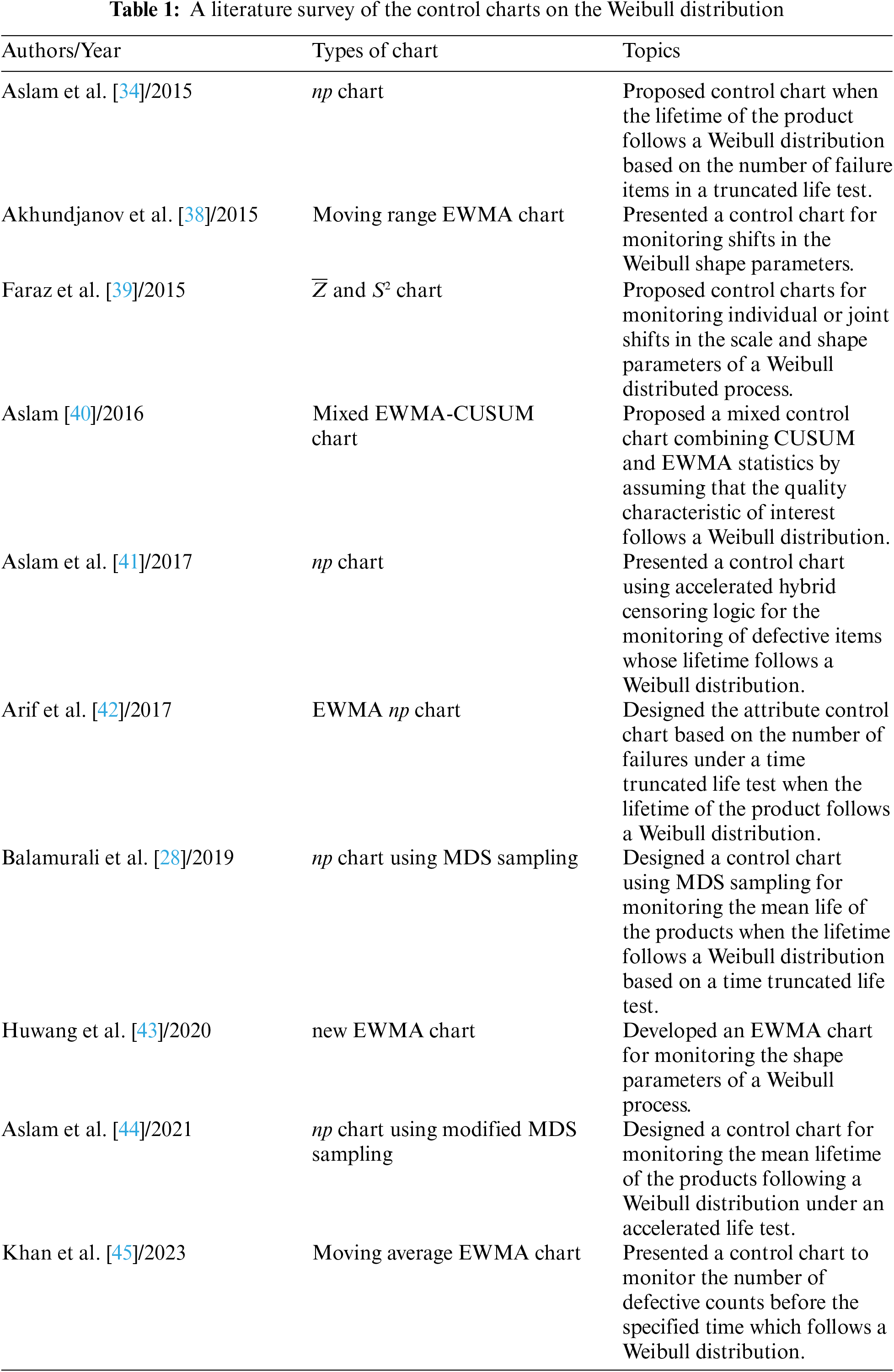
Table 1 shows that researchers applied the Weibull distribution to the attributed control chart to monitor the number of failures or mean life of products under a time truncated life test when the lifetime of the product follows a Weibull distribution. For the variable control chart, the Weibull distribution is often used to monitor variation in the manufacturing process because of the flexible selection of shape and scale parameters. Therefore, this research designs the modified DS np chart using GMDS sampling to monitor the mean life of the product based on the time truncated life test under the Weibull distribution. Let t represent the product lifespan under the Weibull distribution, so the cumulative distribution function can be expressed as follows:

F(t,λ,δ)=1−e(−(tλ))δ,t≥0,λ>0,δ>0,(1)

where λ is a scale parameter that is not known and δ is the known shape parameter. According to the Weibull distribution, the average product lifespan is as follows:

μ=(λδ)Γ(1δ)(2)

Let Γ(⋅) be the complete gamma function. In Eq. (3), under the Weibull distribution, the probability of a given item failing before the experiment time t0 is shown:

p=1−e(−(t0λ))δ.(3)

The value of t0 can be represented as t0=aμ0 for an experiment termination ratio of a using the specific mean lifetime μ0. Consequently, the following can be used to rewrite Eq. (4):

p=1−e−aδ(μ0μ)δ(1δΓ(1δ))δ.(4)

If the process mean is the same as the target mean, or μ=μ0, the process is said to be in-control. Eq. (5) thus becomes:

p0=1−e−aδ(1δΓ(1δ))δ,(5)

where p0 represents the probability of a given item failing. If the process means changes from the target mean, this indicates that the process is out-of-control, shown as μ=fμ0 where f is a shift constant. Next, p1 represents the probability of a given item failing when a process is out-of-control, which has the following equation:

p1=1−e−aδ(1f)δ(1δΓ(1δ))δ,(6)

From Eq. (6), we obtain the probability of a given item failing when there is a shift in process in terms of the specified values of δ, a and f under the Weibull distribution.

2.2 Design of the Modified DS np Chart Using GMDS Sampling

The following section presents the modified DS np control chart using GMDS sampling to monitor the mean life of the product created on the basis of time truncated life tests under the Weibull distribution. The developed control chart includes a pair of inspection stages. In Stage 1, two warning control limits are indicated by LWL and UWL, while the inner control limit is denoted as UCL1. In Stage 2, there is a single outer control limit indicated as UCL2. If a sample point for Stage 1 lies between LWL and UWL, the process can be considered in-control, whereas sample points found beyond the inner control limit will be indicative of a process that is out-of-control. If sample points are located between UWL and UCL1, it is necessary to take a second sample from the same subgroup, whereupon the process can be considered in-control if these sample points fall within the outer control limit of Stage 2, while k of m previous subgroups were found to be in-control for Stage 1. If this is not the case, the process can be considered out-of-control. The operational process for this modified DS np chart with GMDS sampling based on the time-truncated life test under the Weibull distribution can be seen as follows:

1.    Specify the limits indicated as LWL, UWL, UCL1 and UCL2.

2.    The initial sample, of size n1 should be taken for the production process from each subgroup. The lifespan of the item is tested, where t0 is the experiment time, and the nonconforming items (d1) prior to t0 are counted.

3.    In Stage 1 (see Fig. 1)

If LWL≤d1≤UWL, the process can be considered in-control, then return to Step 2.

If d1>UCL1, the process can be considered out-of-control.

If UWL<d1≤UCL1, it is necessary to draw a second sample of size n2. The nonconforming items (d2) in the second sample prior to t0 must be counted. Then go to Stage 2.

In Stage 2 (see Fig. 1), if d1+d2≤UCL2 the process can be considered in-control where k of m previous subgroups were found to be in-control for Stage 1 (LWL≤d1≤UWL), then return to Step 2. If this is not the case, it can be determined that the process is out-of-control.

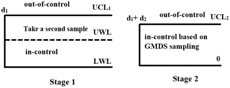
Figure 1: The modified DS np chart based on GMDS sampling procedure

Let d1 and d2 be random variables with binomial distributions with parameters n1, n2 and p0, where p0 is the probability of a given item failing before t0. We can summarize the above steps in a flow chart, as presented in Fig. 2. The modified DS np control chart using GMDS sampling is studied following assumptions and limitations:

1.    The developed control chart monitors the mean life of products under a time-truncated life test when the lifetime of the product follows a Weibull distribution.

2.    The developed control chart is constructed based on a double sampling np chart together with GMDS sampling where p0 follows the Weibull distribution.

3.    At the start of the process, the process is assumed to fit the in-control region, that is μ=μ0.

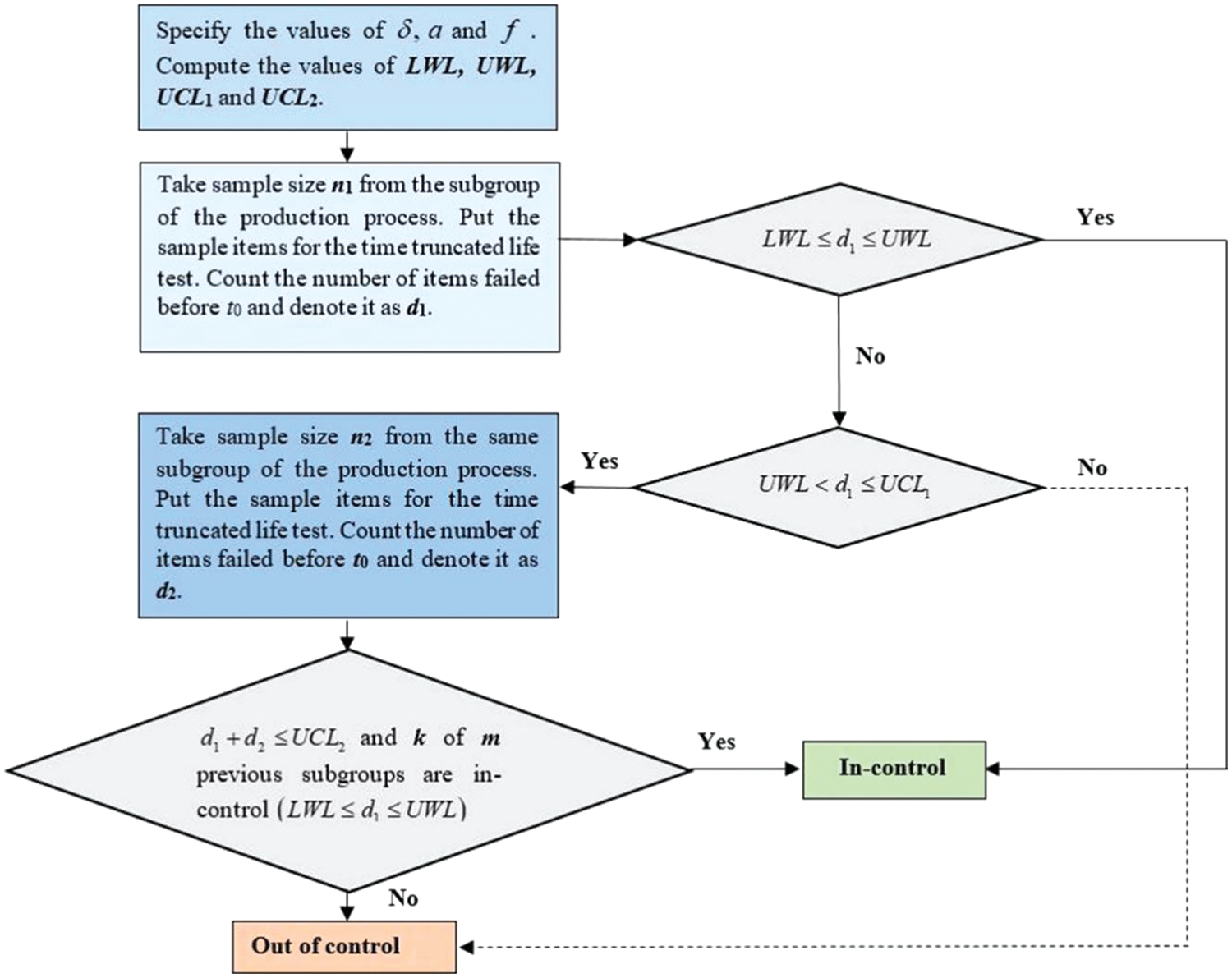
Figure 2: Flowchart of the inspection procedure for the modified DS np chart based on GMDS sampling

The process mean may be shifted to the out-of-control region, that is μ=fμ0.

4.   In this study, the genetic algorithm (GA) with the R program is used to find the optimal parameters.

Therefore, the control limits for Stages 1 and 2 are shown as follows:

Stage 1

UWL=n1p0+wn1p0(1−p0)(7)

LWL=max(0,n1p0−wn1p0(1−p0))(8)

UCL1=n1p0+L1n1p0(1−p0)(9)

Stage 2

UCL2=(n1+n2)p0+L2(n1+n2)p0(1−p0)(10)

where w,L1 and L2 are control limit coefficients with L1>w and L2>0. The developed control chart becomes a DS np chart based on MDS sampling when k=m occurs, while it reduces to a DS np chart if k=m=0 occurs. Similarly, when w=L1=L2 and k=m=0 the developed control chart will reduce to the classical np chart.

Based on the developed control chart, the probability that the process will be considered in-control at Stage 1 is indicated by PS1 and provided as:

PS1(p)=P(LWL≤d1≤UWL)={ ∑d1=⌊ LWL ⌋+1⌊UWL ⌋(n1d1)pd1(1−p)n1−d1 if LWL is not integer∑d1=LWL⌊ UWL ⌋(n1d1)pd1(1−p)n1−d1 if LWL is integer(11)

where ⌊.⌋ is the largest integer that is either less than or equal to the argument. The probability that the second sample is taken from the same subgroup and the total number of nonconforming items in the two samples (d1+d2) is below the outer control limit is represented by PD and expressed as:

PD(p)=P(UWL<d1≤UCL1)×P(d1+d2≤UCL2)=(∑d1=⌊UWL⌋+1⌊UCL1⌋⁡(n1d1)pd1(1−p)n1−d1(∑d2=0⌊UCL2⌋−d1⁡(n2d2)pd2(1−p)n2−d2))(12)

The probability declares that the process is in-control at Stage 2 when given that k of m from the previous subgroup must be in-control at Stage 1, denoted by PS2 and defined as:

PS2(p)=PD×∑j=km⁡(mj)(PS1)j(1−PS1)m−j(13)

According to the modified DS np chart using GMDS sampling, the probability that the process was considered to be in-control is indicated as:

Pin(p)=PS1(p)+PS2(p)=P(LWL≤d1≤UWL)+P(UWL<d1≤UCL1)×P(d1+d2≤UCL2)×∑j=km⁡(mj)(PS1)j(1−PS1)m−j(14)

The probability of declaring that a process is in-control when it is actually in-control (p=p0) can be shown as follows:

Pin(p0)=PS1(p0)+PS2(p0)(15)

Moreover, the probability of declaring that a process is in-control when it is actually out-of-control (p=p1) is obtained as follows:

Pin(p1)=PS1(p1)+PS2(p1)(16)

The ARL0 indicating in-control average run length of the developed control chart is established by:

ARL0=11−Pin(p0).(17)

The ARL1 indicating out-of-control average run length of the developed control chart is determined by:

ARL1=11−Pin(p1).(18)

Additionally, the average sample size (ASS) of the developed control chart for declaring that the process is in-control is provided by:

ASS(p0)=n1+n2P(UWL<d1≤UCL1)(19)

where P(UWL<d1≤UCL1) is the probability of taking a second sample.

2.3 Optimal Design of the Modified DS np Chart Using GMDS Sampling Based on the Weibull Distribution

In this section, we used the following optimization problem to obtain the optimal parameters for constructing the modified DS np chart using GMDS sampling as follows:

MinimizeASS(p0)(20)

Subject to ARL0≥r0,n1<n¯0<n2andn1≤n2,L1>wandL2>0,m>k≥1.

where n¯0 is the pre-determined in-control average sample size. For more details see [14]. The value of ARL was used to assess the performance of the developed control charts. The ASS when the process is in-control was also used to study the performance of the developed control chart. With optimal average sample size, the control charts are more sensitive to detecting process variations. In this study, the genetic algorithm (GA) with the R program is used to find the optimal parameters. The optimal parameters n1, n2, k, m, a and control limit coefficients w, L1, L2 were determined for the specified values of in-control ARL (r0), the shape parameter (δ), and n¯0. For this purpose, we consider r0= 200, 370 and δ= 2, 3, whereas n¯0= 50, 100. All the computations are carried out in the R program. The developed control chart parameters along with ARL are obtained using the following algorithm:

1.    Assign the values of r0, δ and n¯0.

2.    Find out the values of the optimal parameters n1, n2, k, m, a and control limit coefficients w, L1, L2 that result in minimum ASS for which ARL0≥r0 by running the R programming under Eq. (20).

3.    Calculate the ARL1 in Eq. (18) using the optimal parameters n1, n2, k, m, a and control limit coefficients w, L1, L2 from the steps above for various values of the shift constant (f).

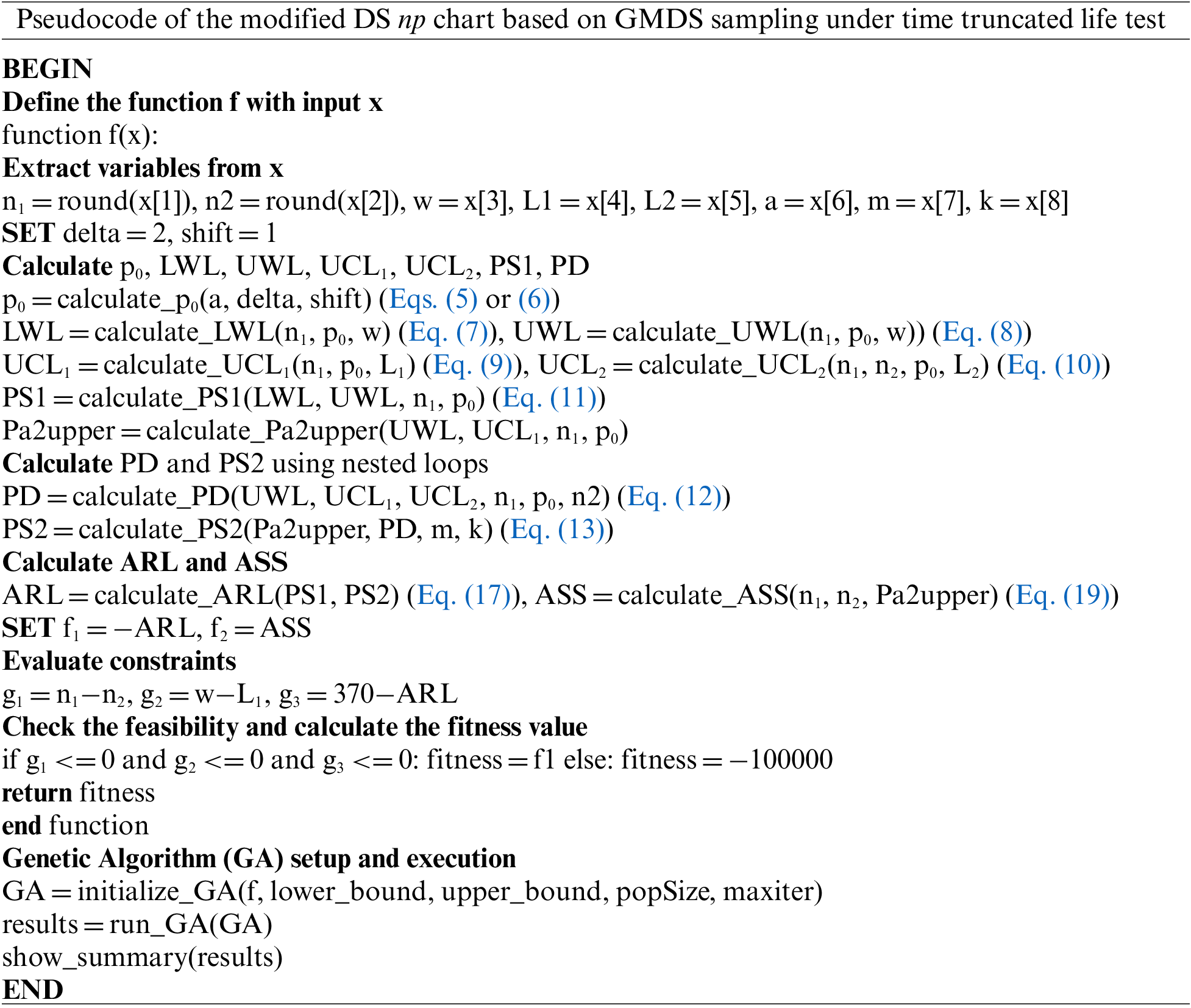
The pseudocode of the modified DS np chart based on GMDS sampling is shown as follows:

3  Results

3.1 Numerical Results

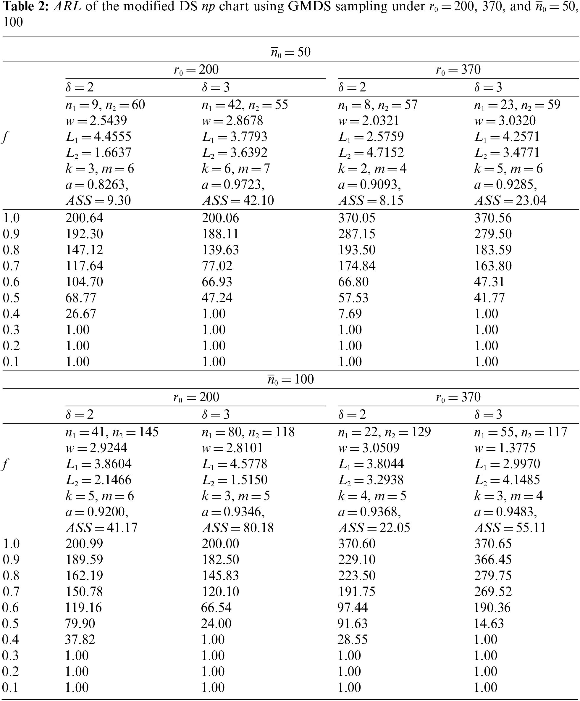
The following section presents the assessment of the performance achieved by the modified DS np chart with GMDS sampling through the use of ARL and ASS. The optimal parameters for the developed control chart (n1,n2,k,m,a) along with the relevant control limit coefficients (w,L1,L2) can be seen in Tables 2 and 3. In establishing the optimal parameters, it is necessary for ARL0 in Eq. (20) to approximate as closely as possible to r0= 200 and 370 for the fixed values of n¯0= 50, 100, and δ= 2, 3. The calculation of ARL1 is made for various values of f under optimal parameters whereby f lies in the range of 1.0 to 0.1. The findings determined from Table 2 can be expressed as shown below:

1.    When δ and n¯0 are fixed, an increase in r0 was linked to a decline in ASS.

2.    When r0 and n¯0 are fixed, an increase in δ leads to an increase in ASS.

3.    It was found that if δ and r0 are fixed, the results show that if n¯0 increases, this will result in ASS also increasing.

4.    As ASS increases, the developed control chart shows greater efficiency in the detection of process shifts. It is also apparent that ARL1 declines to a greater extent in relation to the same shift size. These findings concur with the earlier reports of Adeoti et al. [46].

5.    The findings also indicate a decrease in the values of ARL1 in line with a decrease in shift size.

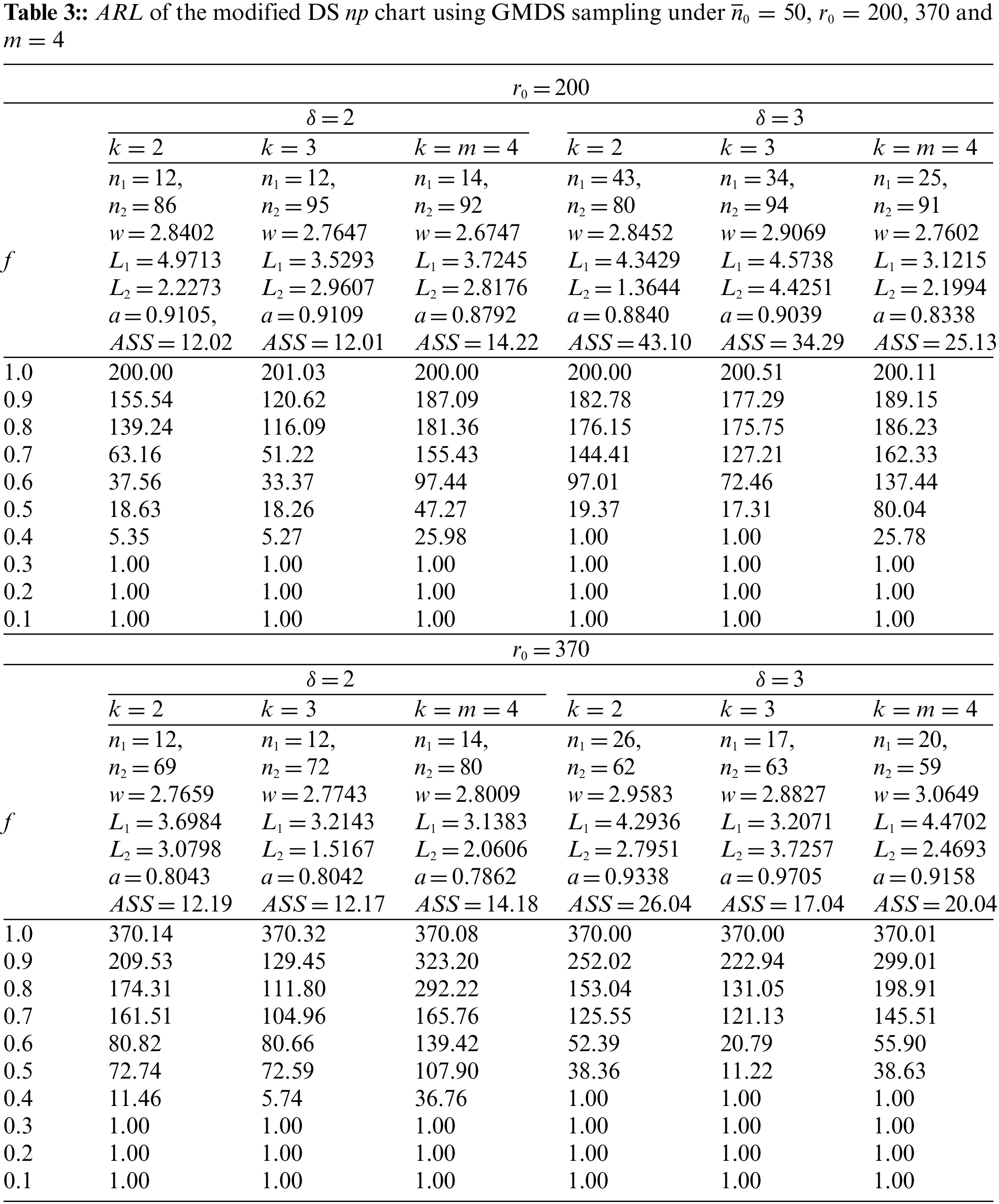
In Table 3, the ARL for the optimal parameters of the modified DS np chart using GMDS sampling can be seen in the context of values for k = 2, 3, 4 and m = 4, where k=m, the developed control chart applying GMDS sampling is reduced to MDS sampling. When the shift size is the same, it can be seen that k = 3 offers the greatest sensitivity in the detection of process shifts, with k = 2 rated slightly lower, while the poorest sensitivity was observed for k=m=4, as may be observed from the ARL1. It can be observed that the developed control chart with GMDS sampling exhibits the lowest ARL1 when k=m−1. No other value of k approaches this result, and the finding concurs with the reported results of [25,26]. This confirms the greater sensitivity in detecting process shifts achieved by the developed control chart with GMDS sampling in comparison to the results for the developed control chart with MDS sampling.

3.2 Sensitivity Analysis

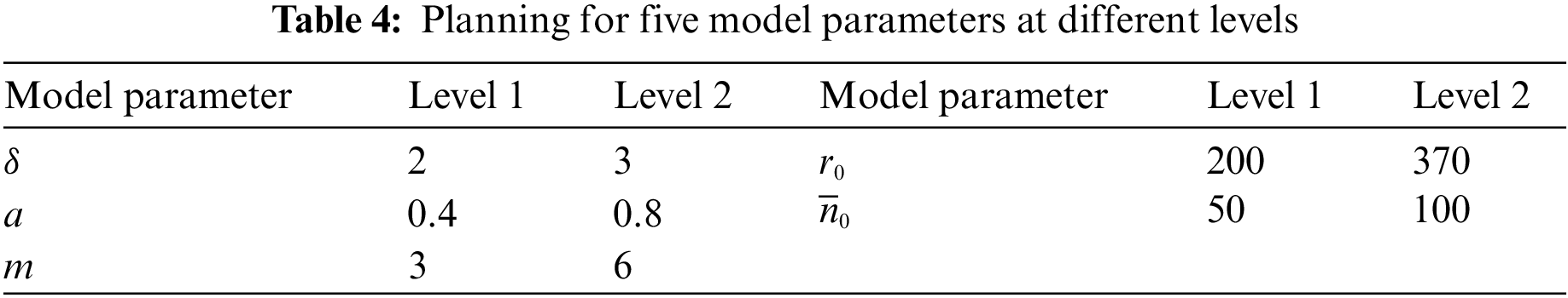
In some cases, the parameters presented in Tables 2 and 3 showed no clear trends or strong correlations. The use of sensitivity analysis can, therefore, help to determine the extent of the influence of these parameters upon the solution from the developed control chart. An orthogonal-array experimental design is used along with multiple linear regression to conduct the sensitivity analysis. For independent variables, the model parameters (a,m,δ,r0, and n¯0) are employed, while the role of the dependent variables is fulfilled by the six test parameters (n1,n2,w,L1,L2, and k) along with ASS and ARL0. The sensitivity analysis tests five model parameters (a,m,δ,r0, and n¯0), for which the corresponding level planning can be observed in Table 4.

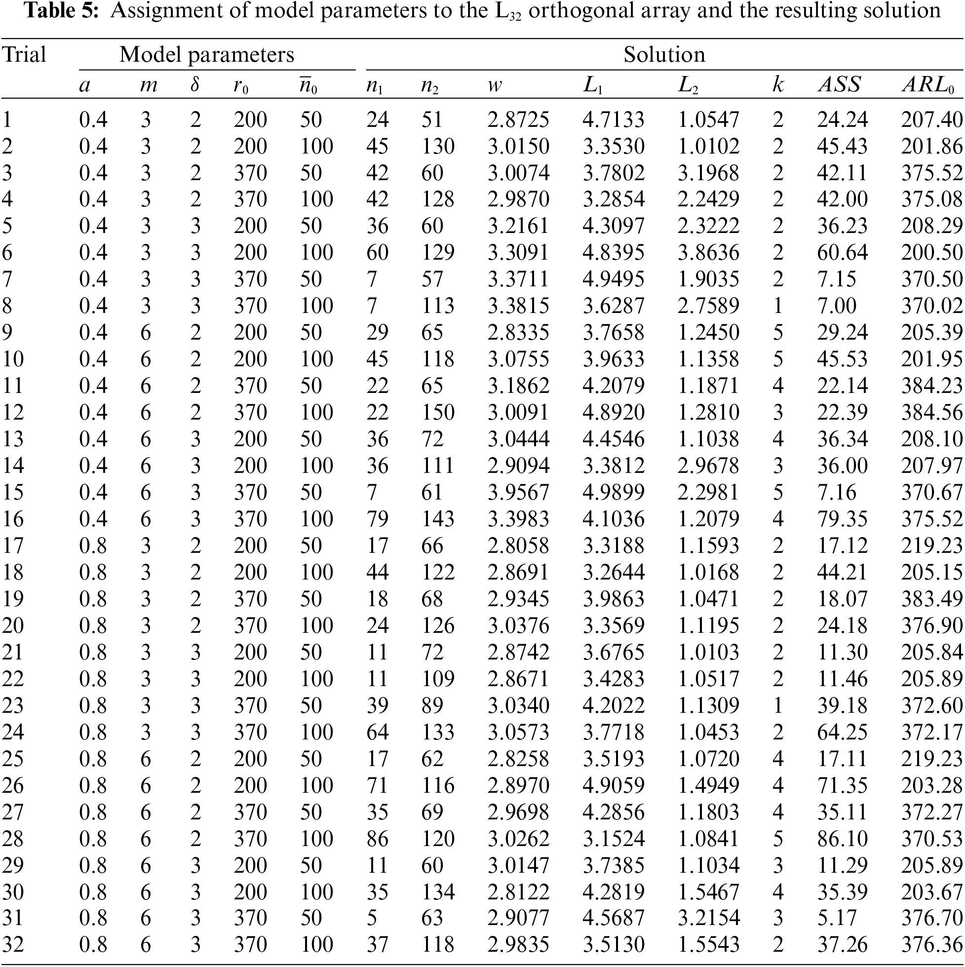
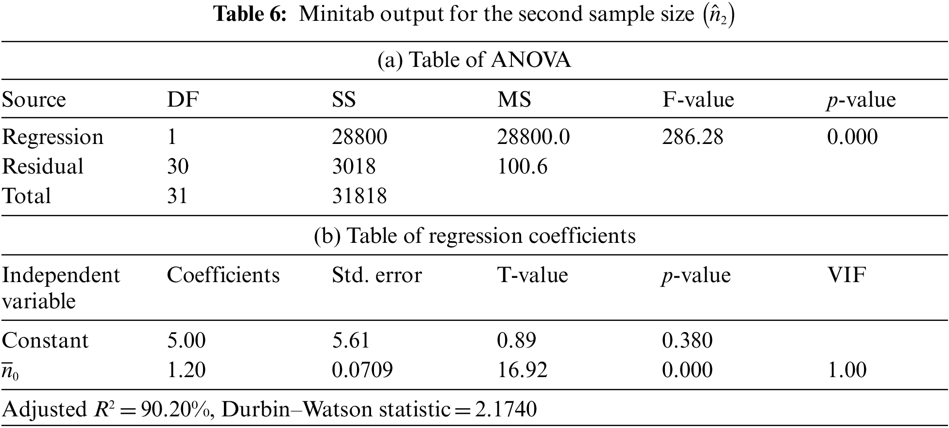
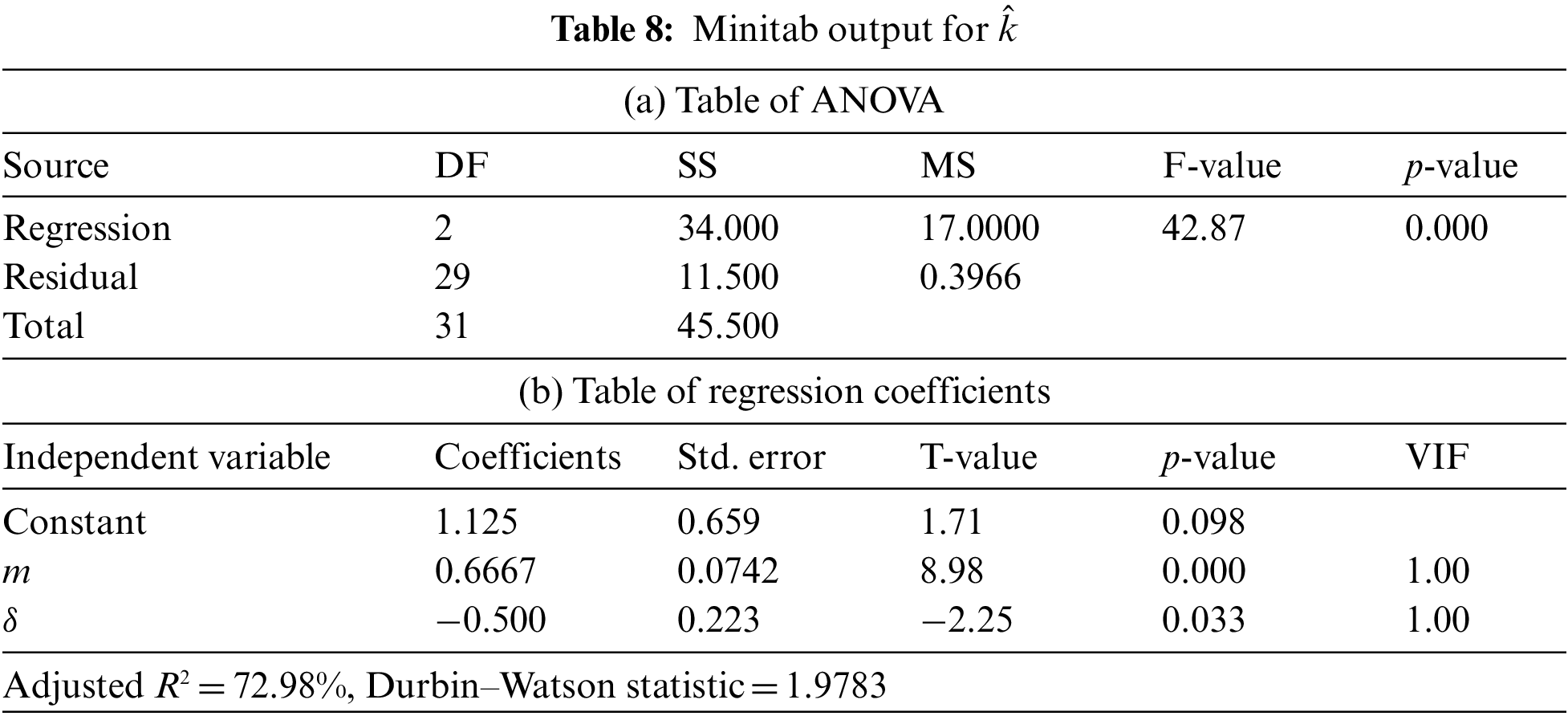
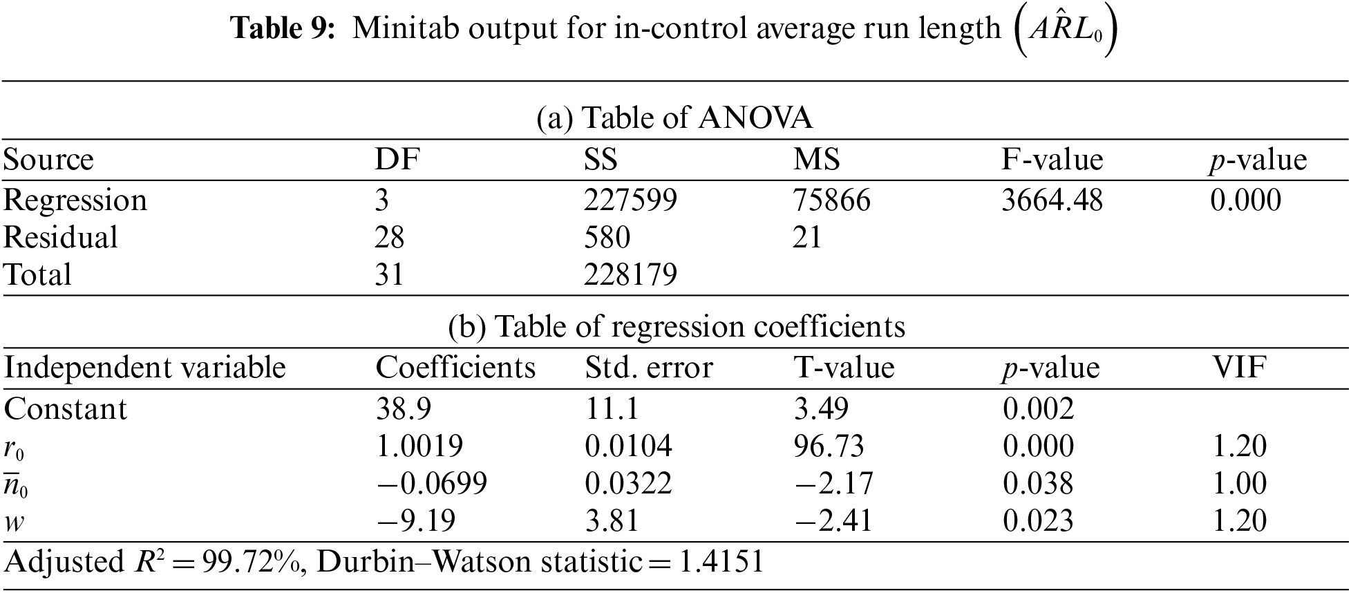
The data shown in Table 5 represents the results from the use of an L32 orthogonal array in the experiment, whereby the five model parameters of the L32 array columns are defined. Accordingly, 32 experiments are required in the L32 orthogonal array experiment design. For the developed control chart, the best solution was produced in each of the trials via GA optimization, which can be seen in Table 5. Multiple linear regression analysis using Minitab 19.0 software was then performed to assess the impact of the various independent parameters on the control chart. ANOVA analysis and multiple linear regression findings for each of the dependent variables are presented in Tables 6–10, and these data can be employed to test statistical hypotheses. Stepwise regression is used to examine the relationships between all values at a significance level of 0.05. The results in Tables 6a–10a indicate that the values of n^2, w^, k^, AR^L0 and AS^S are significantly influenced by at least one of the independent variables. Table 6b reveals that n¯0 influences n^2. Where the coefficient of n¯0 is positive, this is indicative of a relationship whereby increasing n¯0 causes n^2 to increase in turn. Therefore, n¯0 causes n^2 to change by 90.20%.

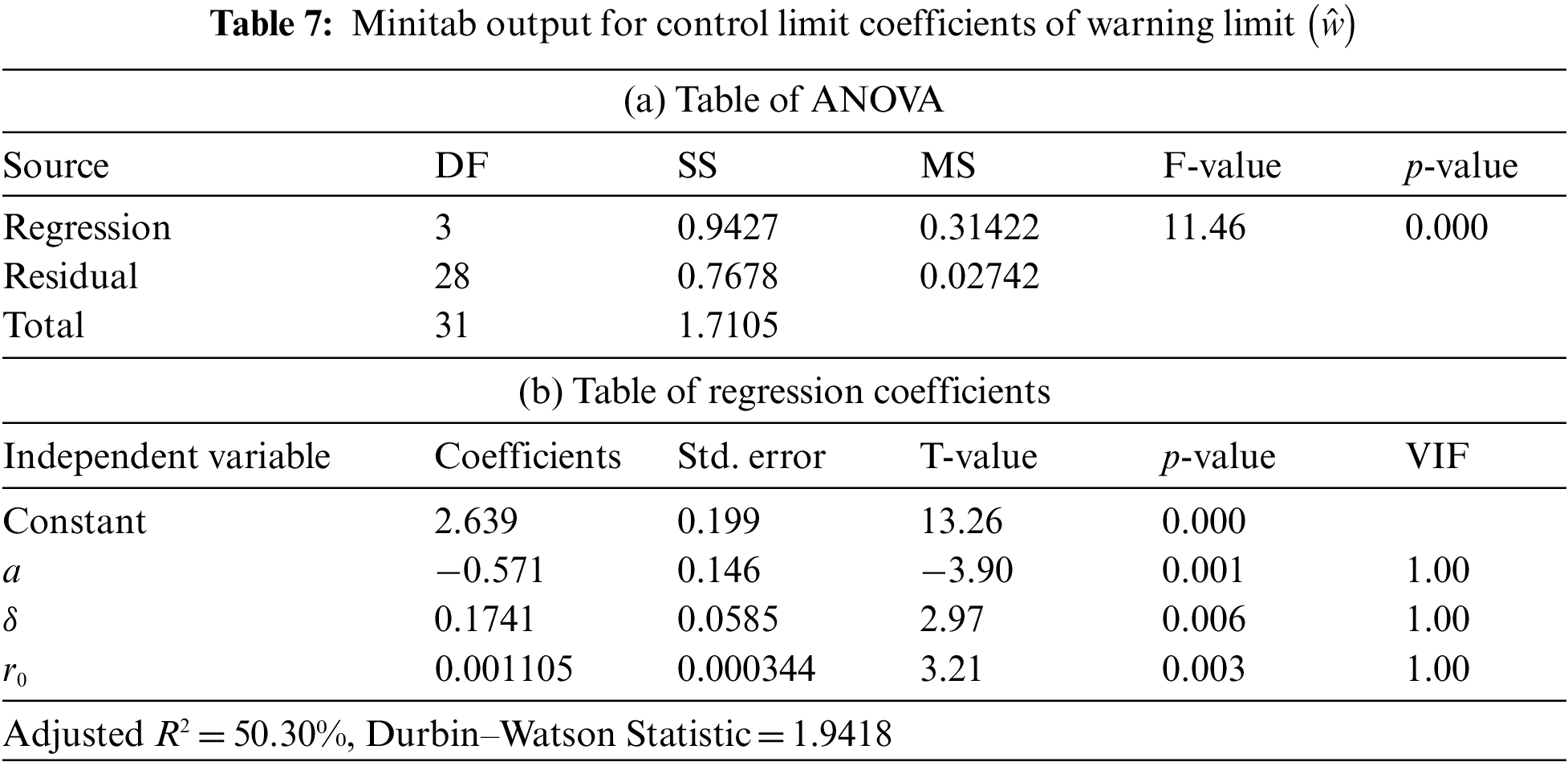
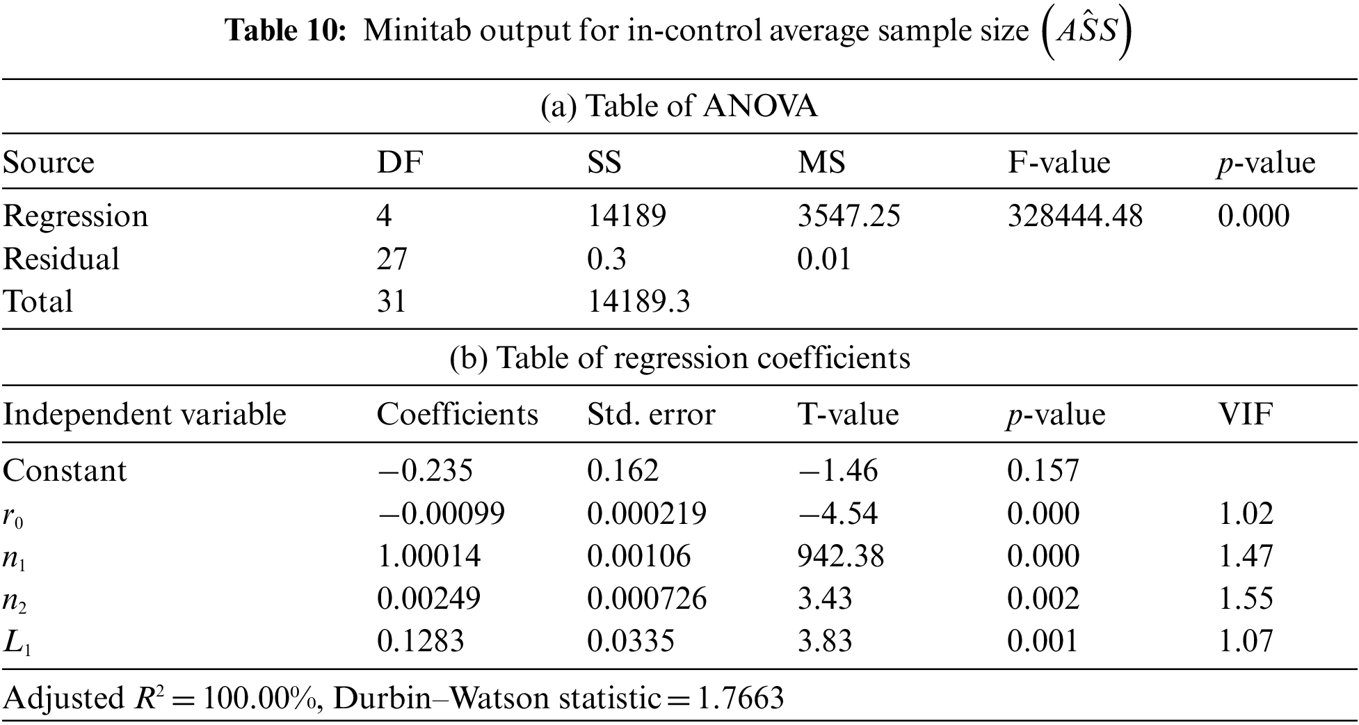
In Table 7b, it can be observed that w^ is influenced by a, δ and r0. Where the coefficients of δ and r0 are positive, this confirms that increasing δ and r0 leads to an increase in w^, whereas a negative coefficient for a shows that increasing a causes w^ to decrease. It is therefore apparent that the effect of a, δ and r0 is to change w^ by 50.30%. The data in Table 8b confirm that k^ is affected by m and δ. Where m has a positive coefficient, this indicates that increasing m results in an increase in k^, whereas a negative coefficient for δ shows that increasing δ causes k^ to decline. It is thus possible to conclude that changes in m and δ will influence k^ by 72.98%. In Table 9b, it is revealed that r0, n¯0 and w have an influence upon AR^L0. Where the coefficients of r0 are positive, this confirms that increasing r0 leads to an increase in AR^L0, while negative coefficients for n¯0 and w confirm that when n¯0 and w increase there will be a corresponding decline in AR^L0. From the data, it is apparent that r0, n¯0 and w have the effect of changing AR^L0 by 99.72%. Meanwhile, Table 10b reveals that r0, n1, n2 and L1 can influence AS^S. Where n1, n2 and L1 have positive coefficients, an increase in n1, n2 and L1 causes AS^S to rise, whereas, in contrast, a negative coefficient for r0 shows that an increase in r0 causes a decline in AS^S. The data show that r0,n1 , n2 and L1 have the effect of changing AS^S by 100.00%.

3.3 Comparative Study

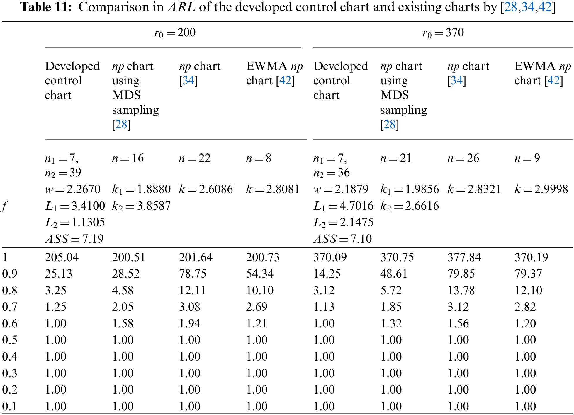
Comparisons are drawn in this section between the performance of the modified DS np chart with GMDS sampling and the control charts of Balamurali et al. [28], Aslam et al. [34] and Arif et al. [42]. The work of Balamurali et al. [28] described an attribute np chart that uses MDS sampling, while the work of Aslam et al. [34] covered an attribute np chart based on single sampling. In addition, the work of Arif et al. [42] presented the design of an attribute EWMA np chart. In all cases, the product lifespan followed a Weibull distribution based on the time-truncated life test. Accordingly, comparisons of the control charts’ performance can be shown using ARLS with identical or similar values for specific parameters of the control charts, such as δ=2, a=0.9, m=3 (for MDS and GMDS sampling), a smoothing constant λ=0.5 (for the EWMA np chart), r0 = 200 and 370. Four control charts were simulated under the same conditions to compare the ARLs. In the case of the developed control chart proposed in this study, the optimization in Eq. (20) uses n¯0=30 and k=2, and pseudocodes of the existing control charts of Balamurali et al. [28], Aslam et al. [34], and Arif et al. [42] are shown as follows:

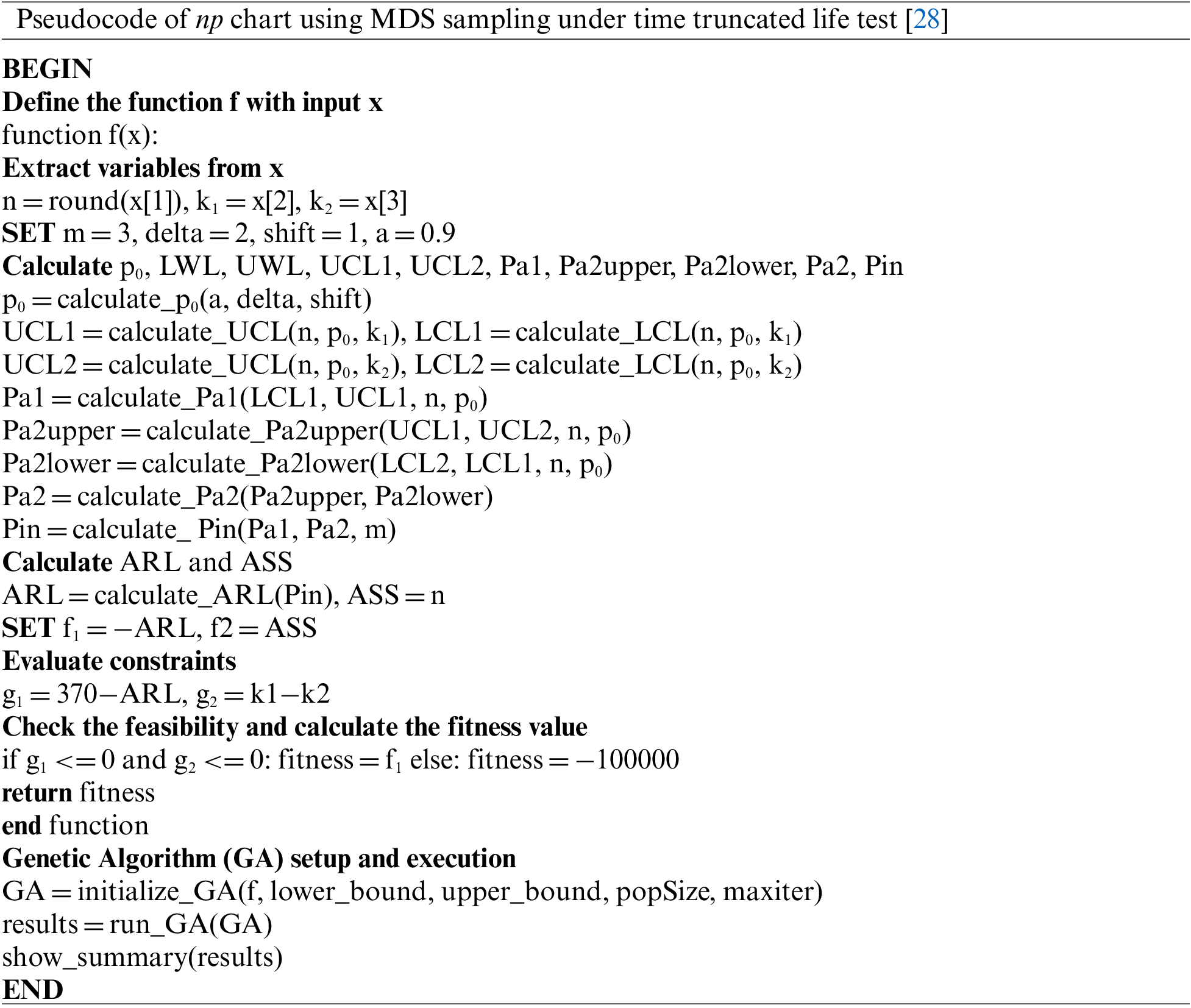
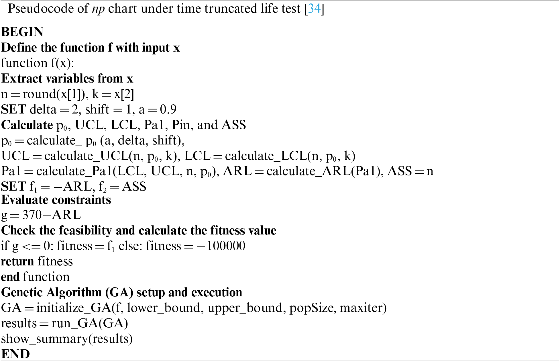
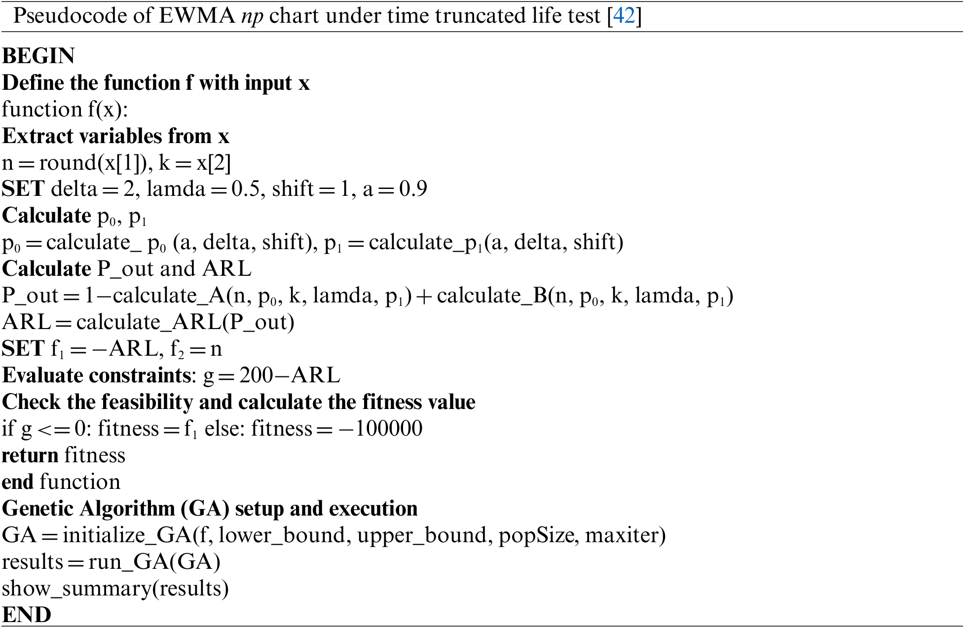
Table 11 presents the optimal parameters at r0 = 200 and 370. The results show that the developed control chart exhibits a smaller ARL1 for every shift size than is the case for those charts presented by [28,34,42]. This confirms that the developed control chart offers greater sensitivity in the detection of small shifts during the process. For instance, when f=0.9, δ=2 and r0=200, the ARL1 value for the developed control chart shown in Table 10 is just 25.13, whereas it is 28.52 for the chart of [28], 78.75 using the chart of [34] and 54.34 from the chart of [42]. Furthermore, the developed control chart made use of average sample sizes (ASS) of just 7.19 in each of the subgroups, whereas the sample size employed by [28] was 16, for [34] the sample size was 22 and the sample size of [42] was 8. In comparison to the existing control charts, the developed control chart can employ smaller sample sizes for each of the subgroups.

4  The Application of the Developed Control Chart Using Real Data

The following section presents the implementation of a modified DS np chart using GMDS sampling in the context of real data concerning the times to failure for 20 aluminum reduction cells where the units are thousands of days [47].

0.4680.7250.8380.8530.9651.5541.6581.7641.7761.1391.9901.1422.0101.3041.3172.2242.2791.4272.2442.286

First of all, the dataset must be examined to determine whether a Weibull distribution is applicable. To check the goodness of fit, the Kolmogorov–Smirnov (K-S) test was used, while the unknown parameters were estimated using the maximum likelihood method. The result for the K-S test is 0.11212, giving a p-value of 0.9391. It can thus be concluded that the data follow the Weibull distribution. Meanwhile, the shape parameter δ^ = 3.0489≈3, while the scale parameter λ^=1.6813. These values were estimated using the maximum likelihood estimate, leading to the value of μ^=1.50. For this research, it can be assumed that δ=3, r0=370, n¯0=50 and μ0=150. The optimal parameters (n1,n2,w,L1,L2,k,m) = (23, 59, 3.0320, 4.2571, 3.4771, 5, 6) are shown in Table 2, while a=0.9285 and ASS=23.04, resulting in the value of p0 from Eq. (5) = 0.4345 while t0=1.3928. Calculation of the control limits for the developed control chart with the optimal values resulted in LWL = 2.79, UWL = 17.20, UCL1 = 20.11, and UCL2 = 51.23. Generation of the initial 20 subgroups used the in-control process (based on a binomial distribution in which p0=0.4345), whereupon the generation of the subsequent 20 subgroups relied upon an out-of-control process making use of the shifted size f=0.9. Finally, the 20 subgroups can be generated based on a binomial distribution in which p1 = 0.5425. In Stage 1, a binomial distribution with the parameters (n1,p0) = (23, 0.4345) is employed for the in-control process while (n1,p1) = (23, 0.5425) is used for the out-of-control process to provide a simulation for the number of nonconforming items d1. Meanwhile, in Stage 2, a binomial distribution with the parameters (n2,p0) = (59, 0.4345) is employed for the in-control process while (n2,p1) = (59, 0.5425) is used for the out-of-control process to provide a simulation for the number of nonconforming items d2. Table 12 presents the simulated data. The values of d1 and d2 are plotted on the developed control chart using GMDS sampling in Fig. 3. It can be seen from Fig. 3 that, at Stage 1, the first 20 subgroups are the in-control process as all the points lie within the warning control limits LWL and UWL. For the next 20 subgroups, the first example of size 23 is taken. Observe that the 35th subgroup has nonconforming items d1=19 whereas the 39th subgroup has nonconforming items d1=18. As d1=18 and 19 falls in the interval UWL<d1≤UCL1 then we go to Stage 2 and take the second sample of size n2=59. For the 35th subgroup, the number of nonconforming d2=31 is observed, and d1+d2= 50 < UCL2 with the result that the process is considered in-control because it meets the requirement that k=5 of the previous m=6 subgroups are in-control processes. Moreover, in the 39th subgroup, it is shown that d1=18, which falls in the interval UWL<d1≤UCL1. At Stage 2, we take a second sample of size n2=59 with d2=27 and obtain d1+d2=45 < UCL2. Then this subgroup result reveals that the process is in-control because it is shown that 5 of the previous 6 subgroups are in-control processes. Fig. 3 clearly shows that the developed control chart declares the process to be in-control.

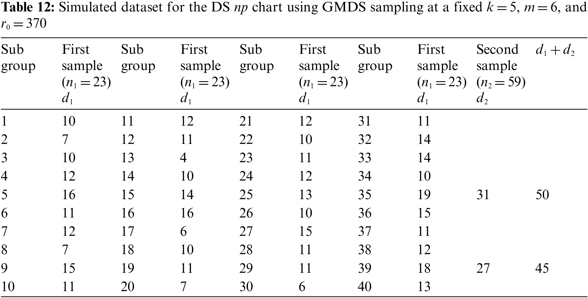
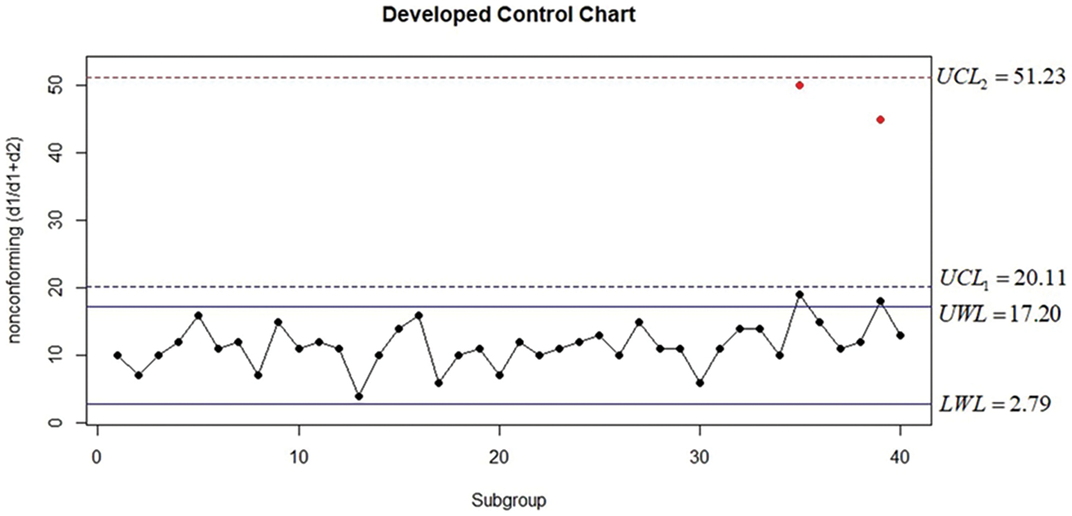
Figure 3: The modified DS np chart using GMDS sampling for simulated data

5  Conclusions

The design of a novel attributed control chart is achieved through the application of the DS np chart combined with GMDS sampling based on a time-truncated life test under the Weibull distribution. The optimal parameters (n1,n2,k,m,a) and control limit coefficients (w,L1,L2) were determined using a genetic algorithm with the R program when r0, δ and n¯0 were fixed. The developed control chart performance was evaluated using the average run length, while the sensitivity analysis was based on an orthogonal experimental design with multiple linear regression. These techniques sought to investigate the influence of the model parameters upon the solution of the developed control chart. The findings revealed that an increased value for n¯0 served to increase n^2. In the case of w^, higher values for δ and r0 tend to increase w^ whereas a higher value for a leads to a decline in w^. For k^, increases in m will increase k^, while in contrast, higher values for δ cause k^ to decrease. Furthermore, increased values for r0 will extend AR^L0, whereas higher values for n¯0 and w lead to a decline in AR^L0. It could also be seen that when the values of n1, n2 and L1 rose, this led to a rise in AS^S, whereas an increase in r0 caused reduced AS^S. The comparative study revealed that the developed chart offered greater sensitivity in terms of the detection of small process shifts than was the case for the previously existing control charts. Furthermore, the developed control chart appears superior in the detection of process shifts when ASS rises and the other parameters remain fixed. The implementation of the developed control chart in this study was based on simulated data which employed parameters taken from the real set of data, thus exhibiting a true measure of the chart’s utility. In conclusion, it can be stated that the developed control chart, which is based on the time truncated lifetime test under a Weibull distribution, offers greater sensitivity in detecting small process shifts as well as utilizing smaller sample sizes than would be necessary with the existing control charts. For future research, a steady-state ARL will be used to evaluate the performance of the proposed control chart based on the Markov chain method for a more accurate assessment. Moreover, neutrosophic statistics will be applied to the proposed control chart when the data comes from a complex process or an uncertain environment.

Acknowledgement: The authors are highly grateful to the reviewers and editors for taking the time to make their comments and suggestions very helpful to the paper.

Funding Statement: This research was supported by the Science, Research and Innovation Promotion Funding (TSRI) (Grant No. FRB660012/0168). This research block grants was managed under Rajamangala University of Technology Thanyaburi (FRB66E0646O.4).

Author Contributions: The authors confirm contribution to the paper as follows: study conception and design: W. Bamrungsetthapong, P. Charongrattanasakul; data collection: P. Charongrattanasakul; analysis and interpretation of results: W. Bamrungsetthapong, P. Charongrattanasakul; draft manuscript preparation: W. Bamrungsetthapong. All authors reviewed the results and approved the final version of the manuscript.

Availability of Data and Materials: The data used in this article are freely available in the cited references.

Conflicts of Interest: The authors declare that they have no conflicts of interest to report regarding the present study.

References

1. Montgomery, D. C. (2009). Introduction to statistical quality control, 9th edition. New York: John Wiley and Sons. [Google Scholar]

2. Gan, F. F. (1993). An optimal design of cusum control charts for binomial counts. Journal of Applied Statistics, 20(4), 445–460. https://doi.org/10.1080/02664769300000045 [Google Scholar] [CrossRef]

3. Gan, F. F. (1990). Monitoring observations generated from a binomial distribution using modified exponentially weighted moving average control chart. Journal of Statistical Computation and Simulation, 37, 45–60. https://doi.org/10.1080/00949659008811293 [Google Scholar] [CrossRef]

4. Epprecht, E. K., Costa, A. F. B. (2001). Adaptive sample size control charts for attributes. Quality Engineering, 13(3), 465–473. https://doi.org/10.1080/08982110108918675 [Google Scholar] [CrossRef]

5. Luo, H., Wu, Z. (2002). Optimal np control charts with variable sample sizes or variable sampling intervals. Economic Quality Control, 17(1), 39–61. https://doi.org/10.1515/EQC.2002.39 [Google Scholar] [CrossRef]

6. Croasdale, R. (1974). Control charts for a double-sampling scheme based on average production run lengths. International Journal of Production Research, 12(5), 585–592. https://doi.org/10.1080/00207547408919577 [Google Scholar] [CrossRef]

7. He, D., Grigoryan, A. (2003). An improved double sampling s chart. Economic Quality Control, 41(12), 2663–2679. https://doi.org/10.1080/0020754031000093187 [Google Scholar] [CrossRef]

8. Costa, A. F. B., Claro, F. A. E. (2008). Double sampling X¯ control chart for a first-order autoregressive moving average process model. The International Journal of Advanced Manufacturing, 39, 521–542. https://doi.org/10.1007/s00170-007-1230-6 [Google Scholar] [CrossRef]

9. Torng, C. C., Lee, P. H. (2009). The performance of double sampling control charts under non-normality. Communication in Statistics—Simulation and Computation, 38(3), 541–557. https://doi.org/10.1080/036109108025711 [Google Scholar] [CrossRef]

10. Khoo, M. B. C., Lee, H. C., Wu, Z., Chen, C. H., Castagliola, P. (2010). A synthetic double sampling control chart for the process mean. IIE Transactions, 43(1), 23–38. https://doi.org/10.1080/0740817X.2010.491503 [Google Scholar] [CrossRef]

11. De Araújo Rodrigues, A. A., Epprecht, E. K., de Magalhaes, M. S. (2011). Double sampling control charts for attributes. Journal of Applied Statistics, 38(1), 87–112. https://doi.org/10.1080/02664760903266007 [Google Scholar] [CrossRef]

12. Chong, Z. L., Khoo, M. B. C., Castagliola, P. (2014). Synthetic double sampling np control chart for attributes. Computers & Industrial Engineering, 75, 157–169. https://doi.org/10.1016/j.cie.2014.06.016 [Google Scholar] [CrossRef]

13. Zhou, W., Wan, Q., Zheng, Y., Zhou, Y. (2017). A joint-adaptive np control chart with multiple dependent state sampling scheme. Communications in Statistics—Theory and Methods, 46(14), 6967–6979. https://doi.org/10.1080/03610926.2015.1132323 [Google Scholar] [CrossRef]

14. Lee, M. H., Khoo, M. B. C. (2021). Double sampling np chart with estimated process parameter. Communications in Statistics—Simulation and Computation, 50(8), 2232–2250. https://doi.org/10.1080/03610918.2019.1599017 [Google Scholar] [CrossRef]

15. Wortham, A. W., Baker, R. C. (1976). Multiple deferred state sampling inspection. International Journal of Production Research, 14(6), 719–731. https://doi.org/10.1080/00207547608956391 [Google Scholar] [CrossRef]

16. Nadi, A. A., Gildeh, B. S. (2019). A group multiple dependent state sampling plan using truncated life test for the Weibull distribution. Quality Engineering, 31(2), 1–11. https://doi.org/10.1080/08982112.2018.1558250 [Google Scholar] [CrossRef]

17. Aslam, M., Jeyadurga, P., Balamurali, S., Azam, M., Al-Marshadi, A. (2021). Economic determination of modified multiple dependent state sampling plan under some lifetime distributions. Journal of Mathematics, 2021, 1–13. https://doi.org/10.1155/2021/7470196 [Google Scholar] [CrossRef]

18. Charongrattanasakul, P., Bamrungsetthapong, W., Kumam, P. (2022). A novel multiple dependent state sampling plan based on time truncated life tests using mean lifetime. Computers, Materials & Continua, 73(3), 4611–4626. https://doi.org/10.32604/cmc.2022.030856 [Google Scholar] [CrossRef]

19. Charongrattanasakul, P., Bamrungsetthapong, W., Kumam, P. (2023). Designing adaptive multiple dependent state sampling plan for accelerated life tests. Computer Systems Science and Engineering, 46(2), 1631–1651. https://doi.org/10.32604/csse.2023.036179 [Google Scholar] [CrossRef]

20. Aslam, M., Khan, N., Chi-Hyuck, J. (2014). A multiple dependent state control chart based on double control limits. Research Journal of Applied Sciences, Engineering and Technology, 7(21), 4490–4493. https://doi.org/10.19026/rjaset.7.825 [Google Scholar] [CrossRef]

21. Aslam, M., Azam, M., Khan, N., Chi-Hyuck, J. (2015). A control chart for an exponential distribution using multiple dependent state sampling. Quality & Quantity, 49, 455–462. https://doi.org/10.1007/s11135-014-0002-2 [Google Scholar] [CrossRef]

22. Aslam, M., Nazir, A., Chi-Hyuck, J. (2015). A new attribute control chart using multiple dependent state sampling. Transactions of the Institute of Measurement and Control, 37, 569–576. https://doi.org/10.1177/0142331214549094 [Google Scholar] [CrossRef]

23. Aslam, M., Arif, O. H., Jun, C. H. (2017). A control chart for gamma distribution using multiple dependent state sampling. Industrial Engineering & Management Systems, 16(1), 109–117. https://doi.org/10.7232/iems.2017.16.1.109 [Google Scholar] [CrossRef]

24. Khan, N., Aslam, M. (2019). Design of an EWMA adaptive control chart using MDS sampling. Journal of Statistics and Management Systems, 22(3), 535–555. https://doi.org/10.1080/09720510.2018.1564206 [Google Scholar] [CrossRef]

25. Aslam, M., Raza, M. A., Ahmad, L., Jun, C. H. (2019). Design of a t-chart using generalized multiple dependent state sampling. Quality and Reliability Engineering, 35(6), 1789–1802. https://doi.org/10.1002/qre.2475 [Google Scholar] [CrossRef]

26. Raza, M. A., Aslam, M. (2019). Design of control charts for multivariate poisson distribution using generalized multiple dependent state sampling. Quality Technology and Quantitative Management, 16(6), 629–650. https://doi.org/10.1080/16843703.2018.1497935 [Google Scholar] [CrossRef]

27. Balamurali, S., Jeyadurga, P. (2019). An attribute np control chart for monitoring mean life using multiple deferred state sampling based on truncated life tests. International Journal of Reliability, Quality and Safety Engineering, 26(1), 1–18. https://doi.org/10.1142/S0218539319500049 [Google Scholar] [CrossRef]

28. Balamurali, S., Jeyadurga, P. (2019). Economic design of an attribute control chart for monitoring mean life based on multiple deferred state sampling. Applied Stochastic Models in Business and Industry, 35(3), 893–907. https://doi.org/10.1002/asmb.2419 [Google Scholar] [CrossRef]

29. Aslam, M., Khan, N., Albassam, M. (2019). Shewhart attribute and variable control charts using modified multiple dependent state sampling. Symmetry, 11(1), 1–14. https://doi.org/10.3390/sym11010053 [Google Scholar] [CrossRef]

30. Aslam, M., Balamurali, S., Periyasamypandian, J., Khan, N. (2021). Designing of an attribute control chart based on modified multiple dependent state sampling using accelerated life test under Weibull distribution. Communication in Statistics—Simulation and Computation, 50(3), 902–916. https://doi.org/10.1080/03610918.2019.1571606 [Google Scholar] [CrossRef]

31. Woodall, W. H., Saleh, N. A., Mahmoud, M. A. (2023). Equivalences between multiple dependent state sampling, chain sampling, and control chart runs rules. Quality Engineering, 35(1), 142–151. [Google Scholar]

32. Aslam, M., Bantan, R. A., Khan, N. (2019). Design of X-bar control chart using multiple dependent state sampling under indeterminacy environment. IEEE Access, 7(1), 152233–152242. https://doi.org/10.1109/ACCESS.2019.2947598 [Google Scholar] [CrossRef]

33. Khan, N., Ahmad, L., Aslam, M. (2022). Monitoring using X-bar control chart using neutrosophic-based generalized multiple dependent state sampling with application. International Journal of Computational Intelligence Systems, 15, 73. https://doi.org/10.1007/s44196-022-00131-3 [Google Scholar] [CrossRef]

34. Aslam, M., Jun, C. H. (2015). Attribute control charts for the Weibull distribution under truncated life tests. Quality Engineering, 27(3), 283–288. https://doi.org/10.1080/08982112.2015.1017649 [Google Scholar] [CrossRef]

35. Khan, N., Aslam, M., Khan, M. Z., Jun, C. H. (2018). A variable control chart under the truncated life test for a Weibull distribution. Technologies, 6(2), 1–10. https://doi.org/10.3390/technologies6020055 [Google Scholar] [CrossRef]

36. Aslam, M. (2019). Time truncated attribute control chart for the Weibull distribution using multiple dependent state sampling. Communication in Statistics—Simulation and Computation, 48(4), 1219–1228. https://doi.org/10.1080/03610918.2017.1408823 [Google Scholar] [CrossRef]

37. Adeoti, O. A., Gadde, S. R. (2021). Moving average control charts for the Rayleigh and inverse Rayleigh distributions under time truncated life test. Quality and Reliability Engineering, 37(8), 3552–3567. https://doi.org/10.1002/qre.2933 [Google Scholar] [CrossRef]

38. Akhundjanov, S. B., Pascual, F. (2015). Moving range EWMA control charts for monitoring the weibull shape parameter. Journal of Statistical Computation and Simulation, 85(9), 1864–1882. https://doi.org/10.1080/00949655.2014.907574 [Google Scholar] [CrossRef]

39. Faraz, A., Saniga, E. M., Heuchenne, C. (2015). Shewhart control charts for monitoring reliability with Weibull lifetimes. Quality and Reliability Engineering International, 31(8), 1565–1574. https://doi.org/10.1002/qre.1692 [Google Scholar] [CrossRef]

40. Aslam, M. (2016). A mixed EWMA–CUSUM control chart for Weibull-distributed quality characteristics. Quality and Reliability Engineering International, 32(8), 2987–2994. https://doi.org/10.1002/qre.1982 [Google Scholar] [CrossRef]

41. Aslam, M., Arif, O. H., Jun, C. H. (2017). An attribute control chart for a Weibull distribution under accelerated hybrid censoring. PLoS One, 12(3), 1–11. https://doi.org/10.1371/journal.pone.0173406 [Google Scholar] [PubMed] [CrossRef]

42. Arif, O. H., Aslam, M., Jun, C. H. (2017). EWMA np control chart for the Weibull distribution. Journal of Testing and Evaluation, 45(3), 1022–1028. https://doi.org/10.1520/JTE20150429 [Google Scholar] [CrossRef]

43. Huwang, L., Lin, L. W. (2020). New EWMA control charts for monitoring the Weibull shape parameter. Quality and Reliability Engineering International, 36(6), 1872–1894. https://doi.org/10.1002/qre.2663 [Google Scholar] [CrossRef]

44. Aslam, M., Balamurali, S., Jeyadurga, P., Khan, N. (2021). Designing of an attribute control chart based on modified multiple dependent state sampling using accelerated life test under Weibull distribution. Communications in Statistics—Simulation and Computation, 50(3), 902–916. https://doi.org/10.1080/03610918.2019.1571606 [Google Scholar] [CrossRef]

45. Khan, N., Nawaz, M. S., Sherwani, R. A. K., Aslam, M. (2023). Moving average EWMA chart for the weibull distribution. Communications in Statistics—Simulation and Computation, 52(5), 2231–2240. https://doi.org/10.1080/03610918.2021.1901119 [Google Scholar] [CrossRef]

46. Adeoti, O. A., Gadde, S. R. (2022). Attribute control chart for Rayleigh distribution using repetitive sampling under truncated life test. Journal of Probability and Statistics, 2022, 1–11. https://doi.org/10.1155/2022/8763091 [Google Scholar] [CrossRef]

47. Whitmore, G. A. (1983). A regression model for censored inverse Gaussian data. Canadian Journal of Statistics, 11(4), 305–315. https://doi.org/10.2307/3314888 [Google Scholar] [CrossRef]