The Optimization Design of the Nozzle Section for the Water Jet Propulsion System Applied in Jet Skis

1  Introduction

As a complex system, the performance of a water jet propulsion system is related to the inlet duct, rotor, stator, and nozzle. The section from the rotor to the nozzle is of the greatest importance, and their parameters influence each other. A literature review revealed that prior studies have barely discussed the integrated system thoroughly; instead, they typically focus on rotor blades. The system proposed based on the findings of this study can be widely applied to jet skis in the leisure industry and fast vessels with a shallow draft and a small stern space.

Jung et al. [1] established a fluid experiment framework for water jet propulsion systems in 2006 and applied PIV technology to observe the velocity distribution in the suction inlet and nozzle outlet. Arash et al. [2] conducted detailed tests on and computations of the performance of a water jet propulsion system from 2014 to 2018 and discussed the system’s impact on thrust deduction coefficient based on fluid dynamics. Their result proved that water jet propulsion systems were unsuitable for slow vessels as they would lead to poor system efficiency. However, when the Froude number was greater than 1, it would prominently highlight the shortcoming that the heavy weight of a water jet propulsion system will cause the stern to sink further. In Brandner et al. [3], a cavitation investigation of the flow within a generic flush type water-jet inlet has been carried out to identify the principal flow features and a suggested CFD model is provided. CFD simulations are performed by Timur et al. [4] at model and full scales for the high-speed littoral combat ship (LCS) surface combatant, including the effect of water-jet propulsion. The evaluation of forces was based on integration of the stress over the wetted area of the hull and water-jet duct, pump casing, and nozzle. Besides, ITTC (2005) water-jet test procedure (control volume method) was used. Wang et al. [5] studied the physical mechanism of a water layer on the morphological evolution of a transient-pulse high-speed water jet, and the formation conditions and main influencing factors of transient pulsed water jet were obtained. Jiao et al. [6] determined the location and morphological characteristics of underwater suction vortices (USV) by high-speed photography. The presence of USV at the intake of the water jet propulsion pump unit can be clearly determined by analyzing the chaotic dynamic characteristics of a pressure fluctuation signal. Lu et al. [7] applied RANS and the SST k-ω turbulence model to compute the performance of a pump jet propulsion with different advance ratios. The results show that the thrust and the torque are in good agreements with experimental data, and also indicate that the rotor provides the main thrust of the propulsion. Furthermore, the pressure distributions around rotor and stator blades are reasonable, but the existence of tip clearance accounts for the appearance of tip vortex that leads to a further loss in efficiency and a probability of cavitation phenomenon. Park et al. [8] used the multiblocked grid system to simulate the characteristic of the inlet duct of the water jet. The numerical results of surface pressure distributions, velocity vectors, and streamlines clearly captured the vortices induced by the separation along the corner of the side wall, and the location of vortices on the lip was well predicted, in accordance with PIV measurement. Gao et al. [9] applied the k-ε turbulent model combined with the standard wall function to compute an axial flow pump. They compared the difference in the flow field of the rear stator with and without a rotor in the system, including the pressure distribution and axial and tangential velocity. Their results suggest that the performance efficiency of the head with a stator installed is superior to that of a single rotor. Moreover, as tested by Gao et al., the wake vortex of the stator at the leading edge on the back could be prevented to the greatest extent when the clearance between the stator and the rotor center was 112 mm, which is the optimal performance. Furthermore, the wake vortex of the stator at the leading edge on the back would influence the velocity around and behind the stator. The findings of Gao et al. also indicated that the computation result is also approximate to the experimental result, proving that the k-ε turbulent model can completely simulate the flow field when both the rotor and the stator are installed. Hu et al. [10] applied CFD to simulate the stalled flow in the intake duct of a mixed-flow pump. Through outputting the velocity vector near the blade, there was reverse flow at the leading edge of the tip. Their study’s conclusion shows that the k-ε model can precisely capture the subtle variations under the interactions between the intake duct and rotor blade; the computation result was approximate to the experimental result. Wang et al. [11] discussed the performance of a water jet propulsion system with different nozzle sizes, outlet areas, and shapes. The optimal flow velocity (Q/Q0) is obtained through the relationship between the head and the system’s efficiency at different conditions. According to the simulation results using different nozzle outlet shapes, the circular nozzle outlet is best for fluid uniformity and head performance. When the nozzle outlet area is 30% of the inlet area, the rotor and system can have optimal efficiency. When the nozzle outlet area increases, the inlet velocity ratio (IVR) curve will rise gradually; consequently, the head and efficiency decrease. Finally, according to the simulation results using different nozzle contours, the change in shape significantly impacts the system’s performance. A linear contraction shape can lead to optimal system efficiency and the most uniform distribution of axial velocity in the nozzle outlet plane. Wu et al. [12] computed a mixed-flow pump while discussing the nozzle, proposing that at a high flow velocity, the occurrence of the vortex at the nozzle outlet and the growth of the boundary layer in the intake duct can be inhibited. In addition, the computation results of the head and efficiency curve are consistent with the experimental results. Chen et al. [13] discussed the rotor inflow of a water jet propulsion system by changing the length of the intake duct; appropriately increasing the length of the intake duct can slightly reduce the flow velocity at the intake. The high-velocity impact of the fluid with the shaft after it was sucked in could be reduced, and the formation of a vortex upstream could be avoided, thus improving the fluid uniformity in front of the rotor. Jiao et al. [14] discussed the hydraulic characteristics of the inlet passage in the water jet propulsion system with different flow parameters and geometric parameters by a combination of numerical simulation and experimental verification. The results show that the numerical results are in good agreement with the experimental results, and the hydraulic performance of the inlet passage is significantly affected by the inlet velocity ratio. The geometric parameters of the best optimization case in [14] are as follows: the inflow dip angle α is 35°, the length L is 6.38 D0, and the upper lip angle is 4°. The optimal operating conditions are the conditions of IVR 0.69 to 0.87.

The current study simulated and optimized the design of an existing water jet propulsion system (pump-jet system). This study aimed to optimize the nozzle section’s design, particularly discussing the nozzle outlet area and its contour characteristics. Changing the above parameters would affect the features of the rear flow field of the stator, which results in a mutual effect on rotor performance. To quantify all performance evaluations, this study used different indicators, such as head coefficient, flow coefficient, and pump efficiency for comparative analyses and discussion to propose an optimal nozzle design.

2  Research Method

The nozzle designed in this study is an acceleration nozzle, as shown in Fig. 1. Parameters include nozzle length (LD), the inner diameter of the parallel section (Di), inlet sectional area (AE), the sectional area of the parallel section (Ai), and the outlet sectional area (AA). Therein, inner diameter of the parallel section (Di) and sectional area of the parallel section (Ai) varied with shape curvature.

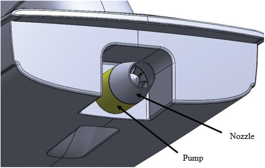
Figure 1: Nozzle installed at the rear part of a water jet propulsion system

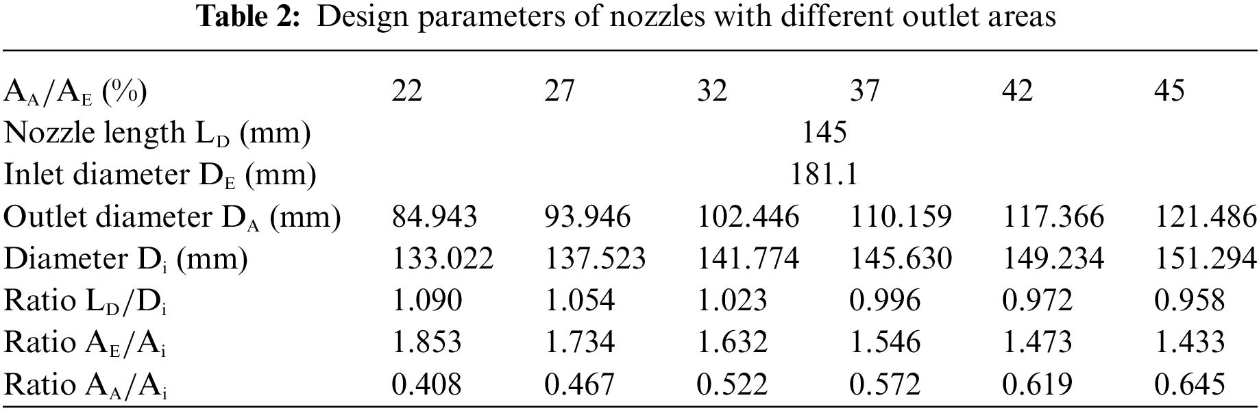
This study adopted the geometrical parameters of the reference nozzle N1 listed in Table 1 as a computation example. Wang et al. [11] divided nozzle geometry into three parts based on the performance of the nozzle of a water jet propulsion system, namely outlet shape, outlet area, and nozzle contour. As mentioned in [11], the nozzle contour is in a linear taper shape or two other different curvature shapes. As mentioned in [11], the outlet shape includes circular, oval, and rounded rectangular shapes, while the outlet area (AA) consists of an increase from 10% of AE to 50% of AE. The reference geometry N1 was not the optimal design and was to be optimized and analyzed in this study. This study referred to the design method of Wang et al. [11] and adjusted the outlet area and changed the nozzle contour based on the existing design dimensions listed in Table 1 to obtain the designs with different outlet areas and nozzle contours. That is, this study first fixed LD and AE, and then changed AA for performance simulation to obtain the optimal AA; then fixed LD,AE,AA of the optimal design, and then modified the nozzle contour. Fig. 2 shows the geometric appearances of linear contraction shape nozzles with different outlet areas. Table 2 lists the design parameters, computed by progressively increasing and decreasing the outlet area by 5% of AE based on the original design area (27%AE).

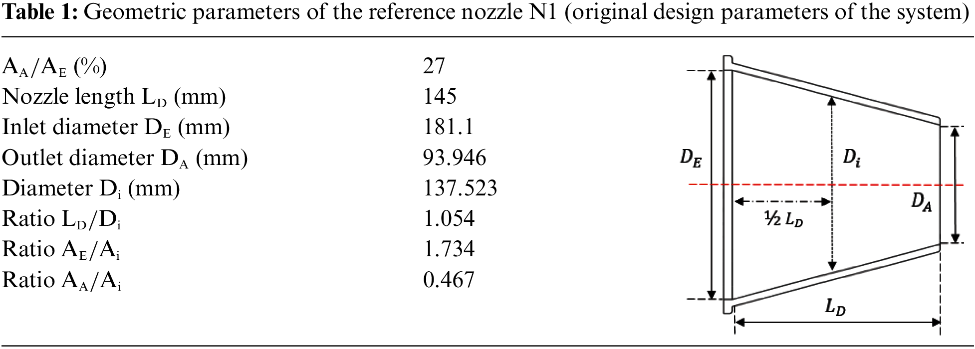
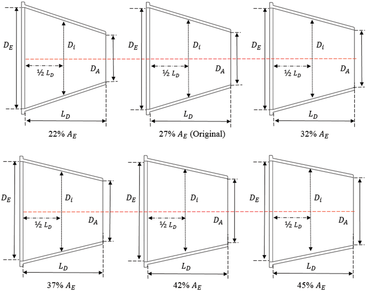
Figure 2: Linear nozzles with different outlet areas

The analysis process of nozzle performance in this study is as follows. First, CFD and the nozzle performance data shown in Fig. 2 were applied to discuss the impacts of outlet area on the system quantity of flow, head, and efficiency to obtain the optimal design area. Then, we fixed the optimal design area but changed the nozzle contour for simulation to discuss the performance of the system with different design shapes and to obtain the optimal design shape for reference. Furthermore, the above discussion must be conducted on the premise that the absorbed horsepower of the rotor and spindle speed is consistent with different outlet areas and nozzle contours. This consistency means that, in each computational combination, the engine is neither overloaded nor under loaded. At the same spindle speed, to maintain a fixed horsepower absorbed by the rotor, the torque of the rotor blade must be the same. In this study, the computational condition was a fixed inflow condition (ship speed) and rotational speed. This condition was obtained from the existing trial result, which was the highest speed of the ship and rotational speed measured using Rotor 27 with a sample stator S1 and nozzle N1 (outlet area 27%AE). Therefore, the rotor torque obtained using this combination was set as the target value (QR*) for rotor pitch adjustment. Taking the outlet area 32% of AE as an example, when the outlet area increases, the flow in the intake duct increases, and the inlet velocity in front of the rotor increases. When the inlet velocity increases, Rotor 27 is used, and the rotational speed remains unchanged; the intake angle of attack of the rotor decreases. This will cause the load and rotor torque to decrease significantly, i.e., the horsepower absorbed decreases. To maintain a fixed horsepower absorbed, the system requires a rotor with a large design pitch ratio to increase absorbed torque. Therefore, the pitch ratio must be increased and computed until the rotor torque reaches the target value using this outlet area. This is also true for other outlet area conditions. The resulting discussion applies only if the pitch ratio of the rotor is adjusted until its torque (QR) remains consistent with the target torque value at the original design outlet area. Fig. 3 shows the nozzle performance analysis flowchart.

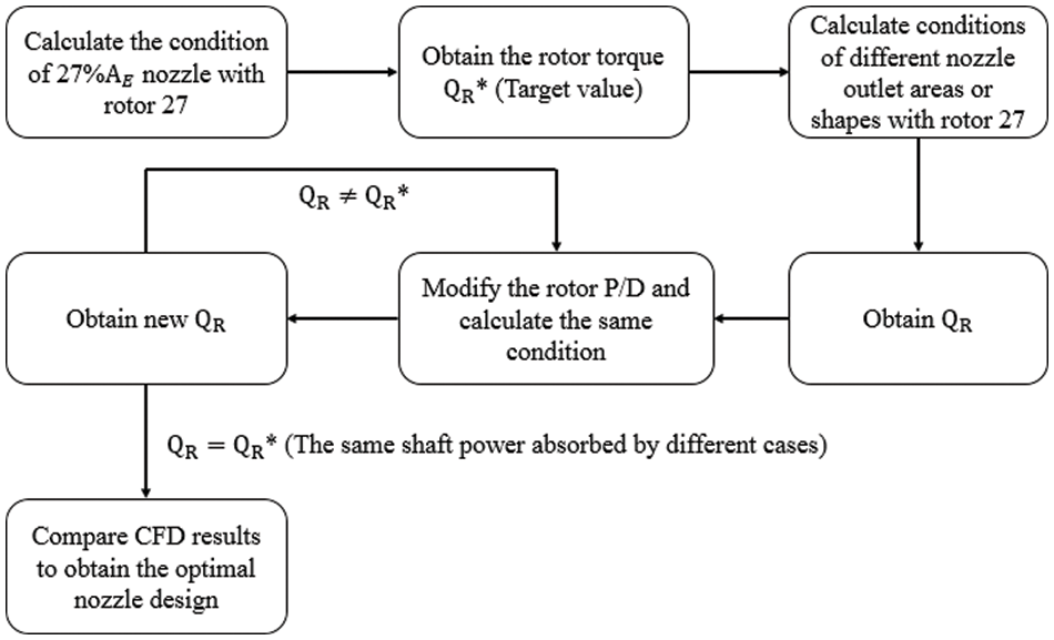
Figure 3: Nozzle performance analysis flowchart

3  CFD Computation Setting

3.1 Turbulence Model and Volume of Fluid (VOF) Method

This study applied CFD to simulate the performance of a water jet propulsion system under the condition that the free surface was included and discussed the difference of the flow field in the intake duct by changing the nozzle’s geometrical parameters. The free surface was computed using the volume of fluid (VOF) method. During computation, fluid was classified into the air and liquid water. The setting of the free surface can be seen in Fig. 4a.

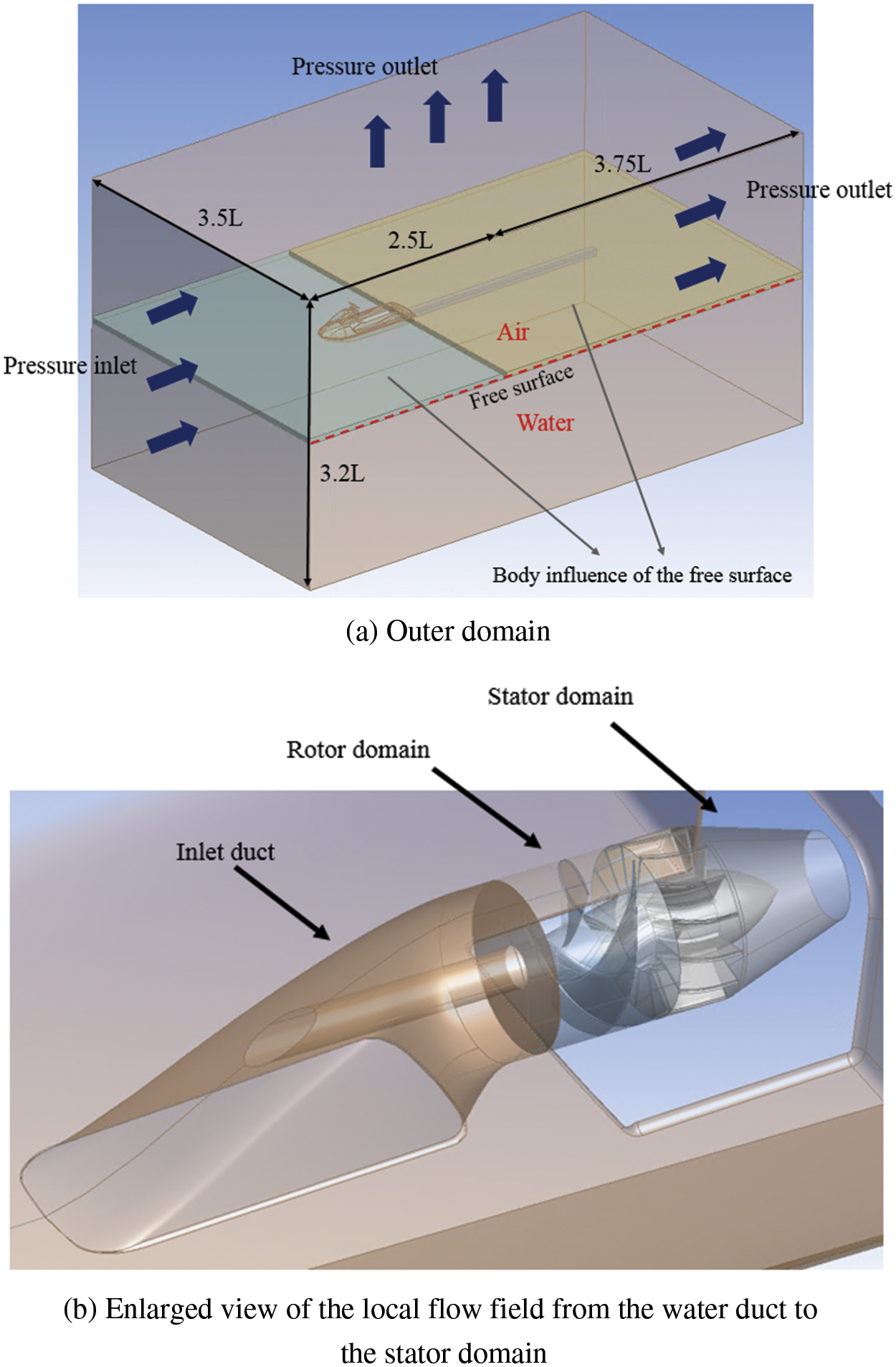
Figure 4: Setting of the computational domain

This study applied the SST k-ω as a turbulence model, which combines the k-ε and k-ω models, and uses a blending function to solve the flow near solid boundaries. The k-ε model is used for the far field and the k-ω model is used for the near wall region. The SST k-ω turbulence model combines the advantages of both models and is adopted for this study.

3.2 Setting of the Computational Domain

This study’s computational domain consisted of three parts: outer and inner domains; the inner domain further consisted of the rotor and stator domains. Fig. 4a shows the outer domain. A large water cube form was used to simulate the fluid space, and a jet ski model was added in the domain. The flow field was built based on the ship’s length of 3.1 m. The rotor center was used as the reference point. The distances between the rotor center, inflow plane, and outflow plane were 2.5 times and 3.75 times the ships’ lengths, respectively. The height and width of the flow field were 3.2 and 3.5 times the ships’ lengths, respectively. The free surface was located 0.12 m above the rotor center, and the meshes are refined by the body influence method. Fig. 4b shows an enlarged view of the local flow field from the water duct to the stator domain. The intake duct included the rotor domain and stator domain of the inner domain. For the rotor domain, the rotor rotation was simulated using sliding mesh. The clearance between the tip and intake duct wall was 0.55 mm. The nozzle shape was the intake duct boundary at the rear part of the stator domain. Regarding the boundary condition setting, the inflow plane in the outer domain was set as the pressure inlet, the top, and the outflow plane were set as the pressure outlet, and the bottom and two sides were set as slip walls. All other boundaries were set as no-slip walls.

3.3 Meshing

Polyhedral meshes are recommend and applied. According to the numerical tests, the application of polyhedral meshes can save at least half of the computing time and the mesh quantity as compared with those of hexahedral and tetrahedral meshes, and the computing results are consistent. This paper focuses on discussing the propulsive performance due to the modifications of the nozzle. Thus, grids in the nozzle are refined. Inside the nozzle, the y+ value on the boundary is under 100, and the side length of the mesh is under 0.006 multiplied by the rotor diameter. However, the micro phenomenon of the flow field at the stern is not discussed in this paper. Though the grids of the boundary layer at the motorboat hull and the water jet passage inlet are not as dense as those inside the nozzle, the inflow at the passage inlet is confirmed to be consistent by the grid independence analysis. Figs. 5 and 6 show the mesh distributions of the nozzle, rotor and stator.

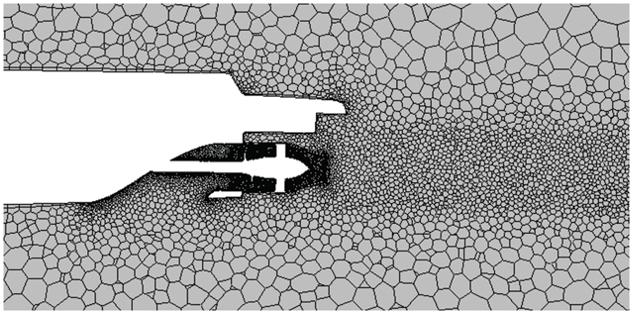
Figure 5: Mesh refinement behind the nozzle

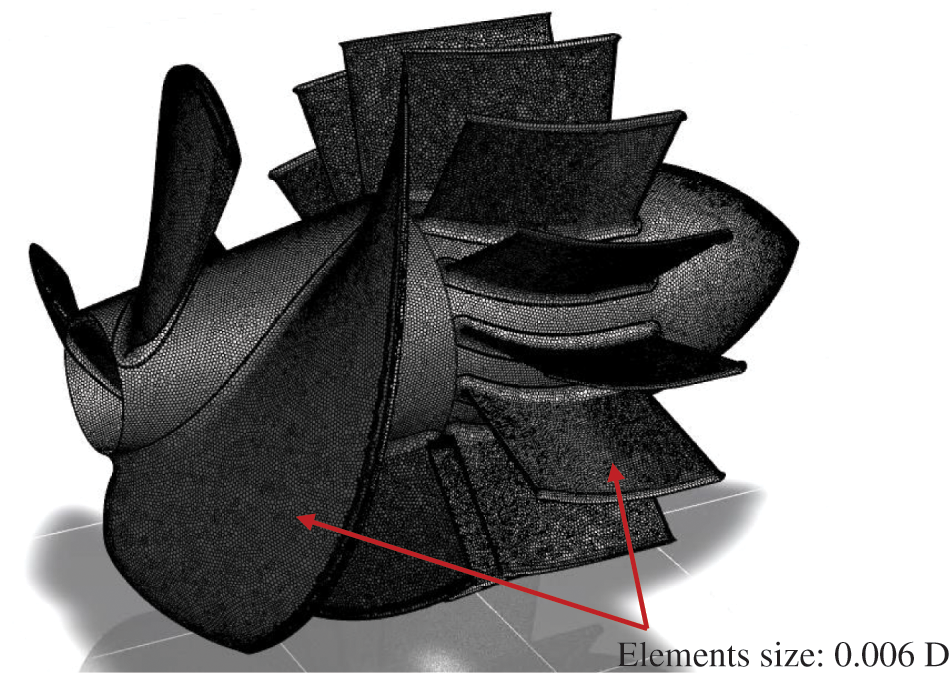
Figure 6: Polyhedral meshes of the rotor and stator

4  Performance Evaluation

This study used different parameters to discuss and evaluate the performance of the water jet propulsion system. Two planes were obtained for further discussion. Plane 1 was captured at the distance 0.5 multiplied by the rotor diameter; Plane 2 was captured at the nozzle outlet, as shown in Fig. 7.

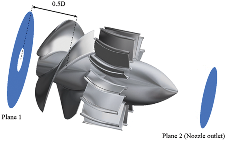
Figure 7: Scheme of the captured planes

The following performance parameters were obtained by outputting the physical quantities on the two planes. The unit of the total head expressed by Eq. (1) is length unit (meter). The parameters shown in Eqs. (2)–(6) are all non-dimensionless.

HT=P2−P1ρg(1)

ψ=gHTn2D2(2)

φ=QnD3(3)

ηt=TnetVA2πnQR(4)

ηp=QρgHT2πnQR(5)

IVR=V1Vs(6)

In Eq. (1), HT is the total head, ρ is the fluid density, and g is the gravitational acceleration. In the calculation of the total head of the system, the total pressure included the impact of static and dynamic pressures. In Eq. (2), the head coefficient ψ was obtained through the non-dimensionalization of the quadratic rotational speed (n) and rotor diameter (D) by HT. In Eq. (3), φ is the flow coefficient, n is the cubic quadratic rotational speed, D is the rotor diameter, and Q is the flow rate. In Eq. (4), ηt is the thrust efficiency (i.e., rotor efficiency), T is the net thrust of the water jet thruster (i.e., rotor thrust or net thrust). The thrust efficiency (Tnet × VA/Shaft Power) can be used to express the propulsion performance. VA is the rotor inlet velocity, and QR is the rotor torque. In Eq. (5), ηp is the pump efficiency and is the ratio of fluid work to shaft work. This study’s discussion was based on the same absorbed horsepower, i.e., the denominator in Eq. (5) was fixed to compare the products of head and flow (HT×Q). The pump efficiency was also a performance indicator, including the interactions between the rotor, stator, and nozzle, i.e., the highest pump efficiency represented the optimal design. In Eq. (6), the inlet velocity ratio IVR was obtained through the non-dimensionalization of ship speed Vs by mean inflow velocity of Plane 1 V1, and had a similar meaning as the (1-W) of the pump. In addition to the parameters mentioned above, this study also outputted flow field pressure, velocity distribution, and other physical phenomena for observing and discussing whether the computations in this study conform to the physical significance.

5  Calculating Condition and Grid Independence Analysis

This study used Rotor 27, stator S1 with the linear nozzle with an outlet area of 27%AE (nozzle N1) for mesh convergence analysis. Table 3 lists the computational conditions. Inlet velocity and rotational speed were trial results.

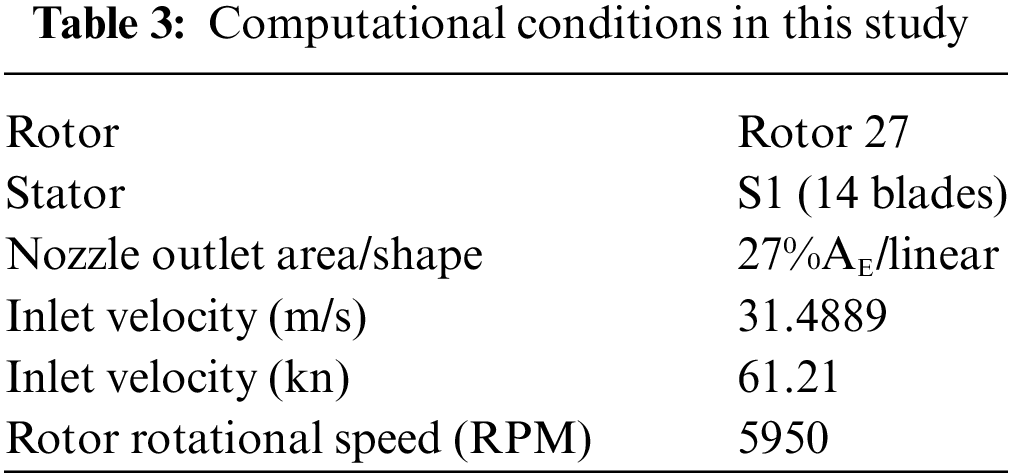
Three physical quantities were outputted for convergence analysis: net thrust, rotor torque, and flow coefficient φ. Table 4 lists the computation results at a different number of polyhedral meshes.

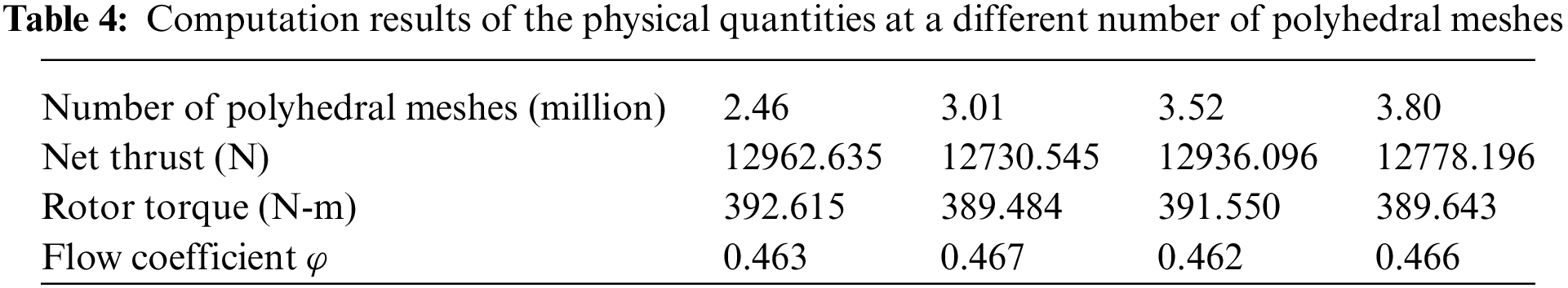
Table 5 and Fig. 8 show the results of the grid independence analysis. The number of meshes increased from 3.52 million to 3.8 million, and the relative errors were less than 1.5%. The relative error of rotor torque and flow quantity was less than 1%, indicating that 3.52 million polygon meshes reached the accurate convergence result. Therefore, this study used 3.52 million polygon meshes number as the basis for analysis.

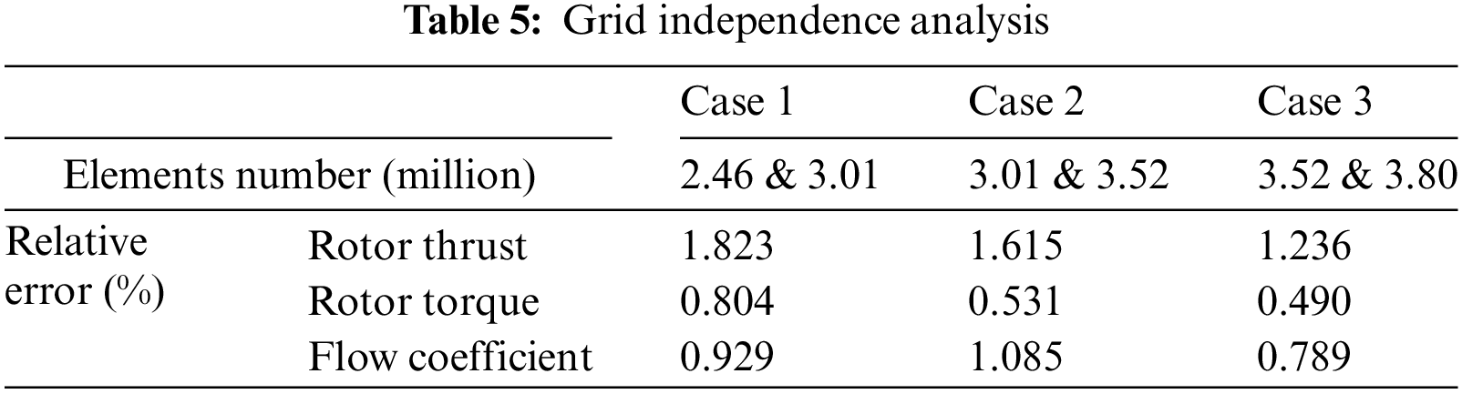
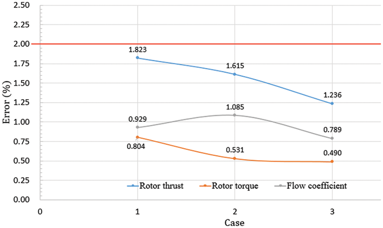
Figure 8: Grid independence analysis

6  CFD Simulation Results of Different Outlet Areas

As shown in Fig. 3, the discussion on nozzle performance should be based on a fixed torque by the rotor in each computation. Therefore, this study first used the existing rotor (Rotor 27), stator S1, and nozzles with different outlet areas for calculations to obtain the rotor torque at the same calculation condition. The torque obtained at the outlet area of 27%AE was the target value in this phase. Except for the outlet area of 27%AE, the rotor pitch ratio was adjusted for other outlet areas to obtain the target absorbed torque.

6.1 Qualitative Discussion

In this study, the nozzle outlet area increased from 22%AE to 45%AE, including the original design 27%AE (N1 nozzle). The detailed descriptions regarding the geometry parameters have been included in Fig. 9. Rotor 27 is a levorotatory rotor. Fig. 2 shows the geometric appearance of nozzles with different outlet areas, and Table 2 lists their design parameters.

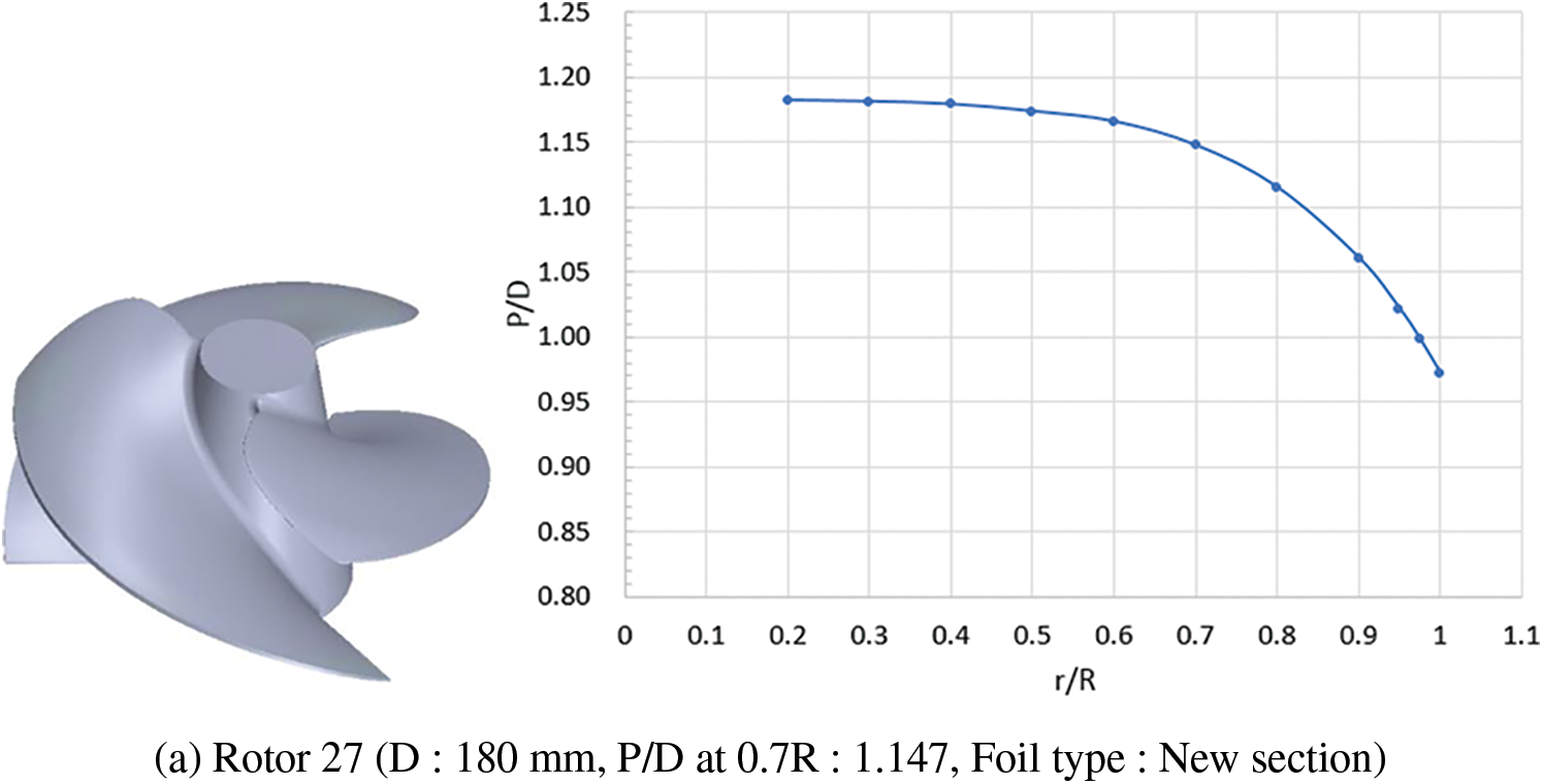
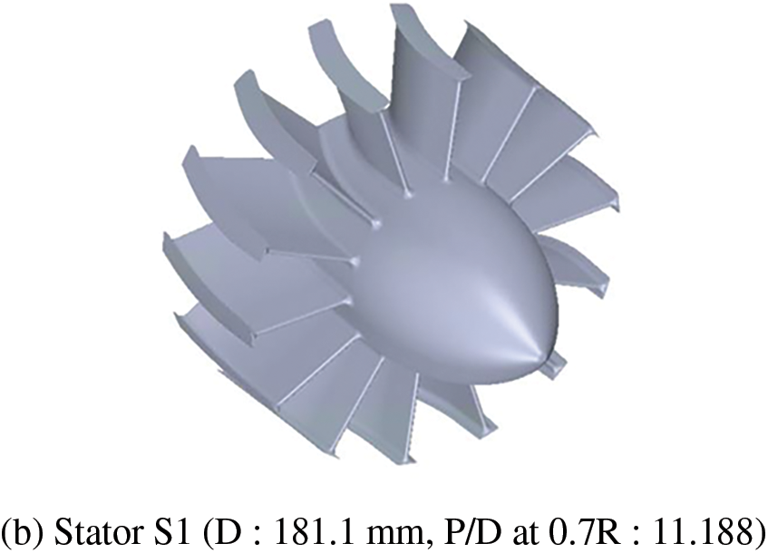
Figure 9: Geometric appearance and parameters of Rotor 27 and stator S1

Table 6 lists the computation results when Rotor 27 was used with nozzles with different design outlet areas. The findings indicate that a change in the outlet area significantly impacted the flow rate. When the outlet area increased, the flow rate increased; the rotor inflow velocity increased, and the outlet velocity decreased (weak jet flow). As a result, when the system uses nozzles with different outlet areas, its head, net thrust, and the performance of rotor torque can vary greatly. When the outlet area increased, the rotor inflow velocity (VA) increased. This indicates that a smaller attack angle of the rotor inflow caused thrust and torque to decrease, thus reducing the head. Fig. 10 shows the dynamic pressure distribution in the flow field when Rotor 27 was used with nozzles with different outlet areas. The figure shows the comparison between the results from the original design area and those from 37%AE (with the area of an 10% increase of the original design). When the outlet area increased, the inlet velocity in front of the rotor increased, and the outlet velocity at the outlet decreased. As a result, the dynamic pressure difference between Planes 1 and 2 decreased. As shown in Fig. 10, at the 37%AE condition, the jet flow intensity in Plane 2 decreased due to a larger outlet area. Therefore, the dynamic pressure in Plane 2 reduced significantly. In addition, the decrease in rotor thrust indicates that the static pressure contributes less to the head. This can be explained by the static pressure distribution in the flow field shown in Fig. 11. The difference in static pressure in front of and behind the rotor at the 37%AE condition significantly reduced compared to the 27%AE condition. This indicates that it is more challenging to lower the pressure of Plane 1 and raise the pressure of Plane 2. This study’s findings indicate that thrust loss lowers the head so the static pressure contributes less to the head. Considering the effects of dynamic and static pressure, a larger outlet area leads to a lower head, as shown in Table 6. The jet stream of a linear nozzle still tends to contract downstream. The head calculated from the position of the linear nozzle outlet may differ from the actual head of the water jet propulsion.

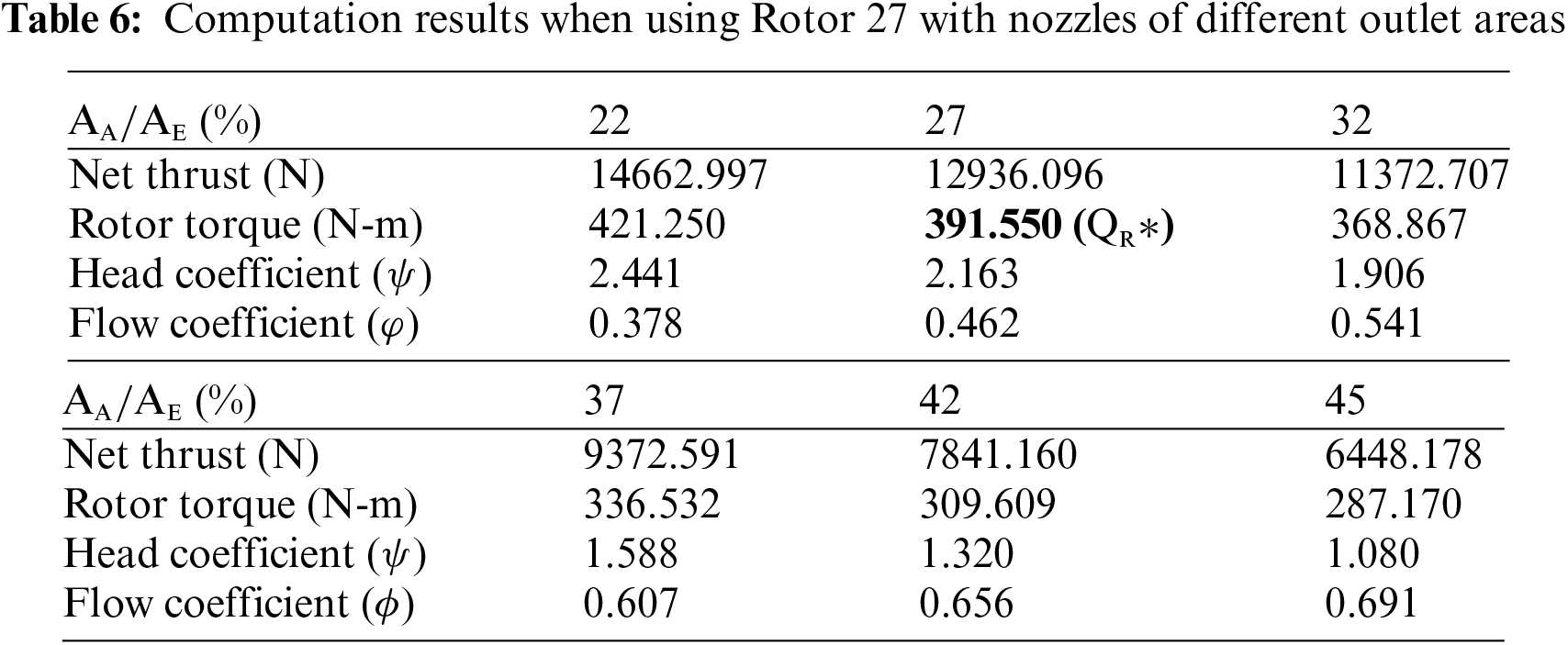
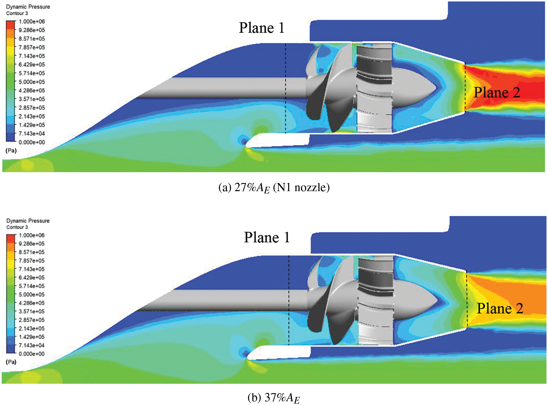
Figure 10: Distribution of dynamic pressure in the flow field when using Rotor 27 with nozzles of different outlet areas

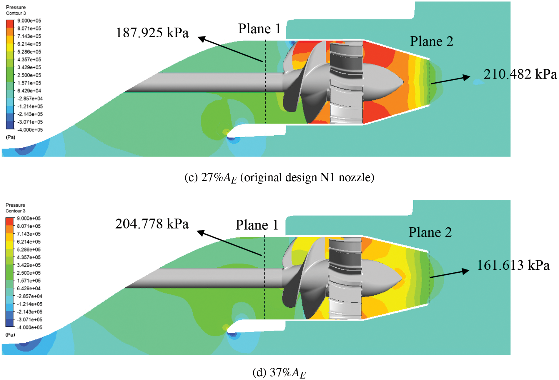
Figure 11: Distribution of static pressure in the flow field when using Rotor 27 with nozzles of different outlet areas

According to the torque values obtained from all computations listed in Table 6, compared to the target value obtained using the original design area, the torque absorbed by the rotor at the 22%AE condition was excessively large. This indicates that the pitch ratio needs to be reduced to make the torque decrease. A larger outlet area will lead to an excessively small torque. Therefore, the pitch ratio can be increased to increase torque.

Fig. 12 shows the axial velocity distribution of all computations in Plane 1. The view of Fig. 12 is looking from the bow to the stern, and at the rotor rotates clockwise. As shown in Fig. 12, all outlet area conditions show significant differences in velocity in areas above and below the shaft in Plane 1. The area below the shaft is approximate to the intake, and fluid is not blocked in this area. Therefore, there is a high-velocity quantity in this area. The area above the shaft is far away from the intake, i.e., fluid will flow along a long path before arriving at this area, during which friction of the intake duct walls and the shaft will block it. Therefore, the velocity in this area is low. Furthermore, at a higher flow rate, a larger outlet area causes the flow velocity in the area below the shaft to be higher due to a significant increase in flow rate. At the same time, the flow velocity in the area above the axis also rises. Fig. 13 shows the distribution of average inlet velocity in different radial positions in Plane 1, namely, the wake distribution. For the 22%AE curve in Fig. 13, a different pattern appears as compared to the others at lower r/R. This difference is caused by the thicker boundary layer due to the lower inflow velocity of the 22%AE condition. Therefore, velocity decreased significantly in the area near the root radial position. At other conditions, the wake distribution trend was similar: velocity increased near the root and decreased towards the tip.

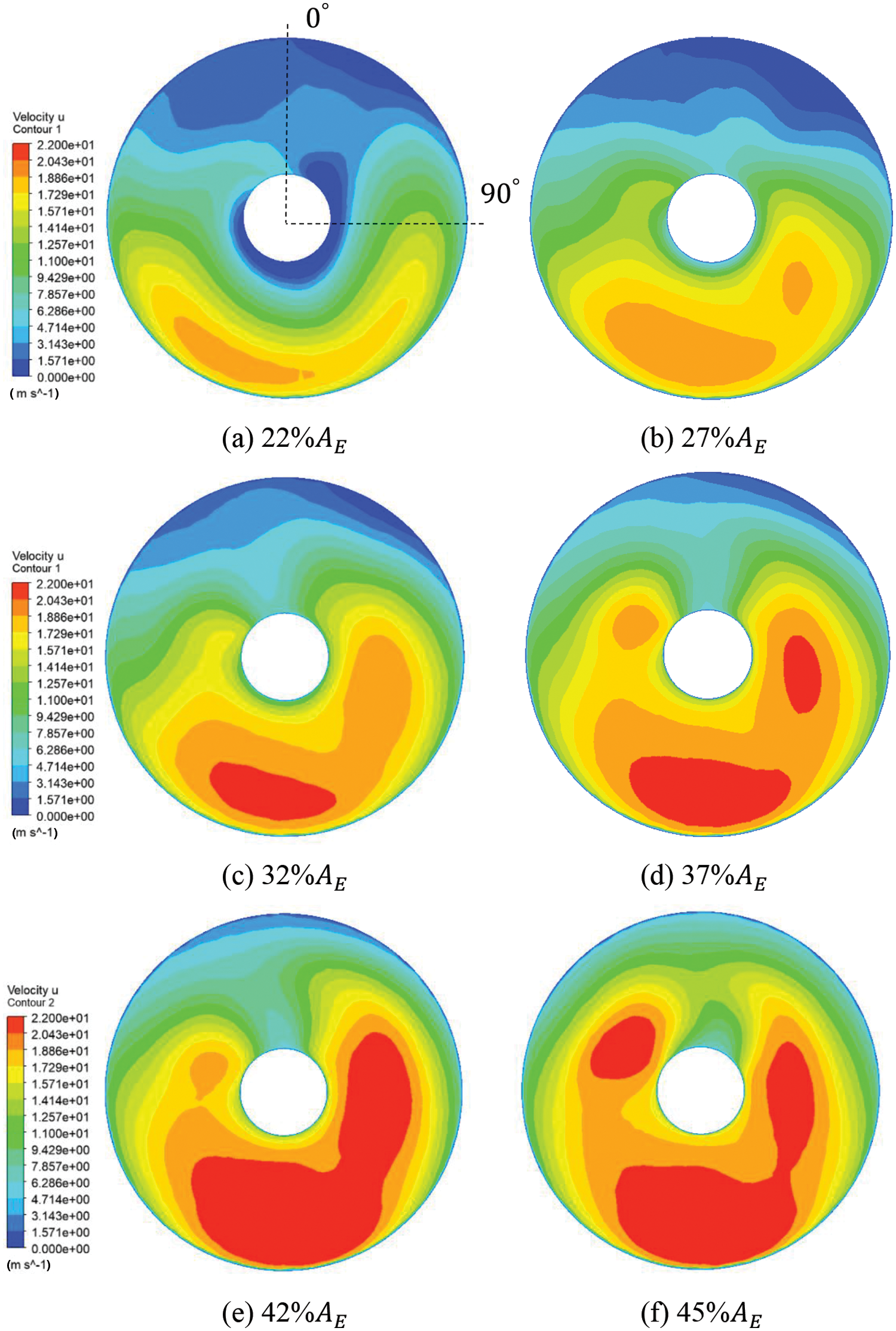
Figure 12: Distribution of axial velocity in Plane 1 when using Rotor 27 with nozzles of different outlet areas

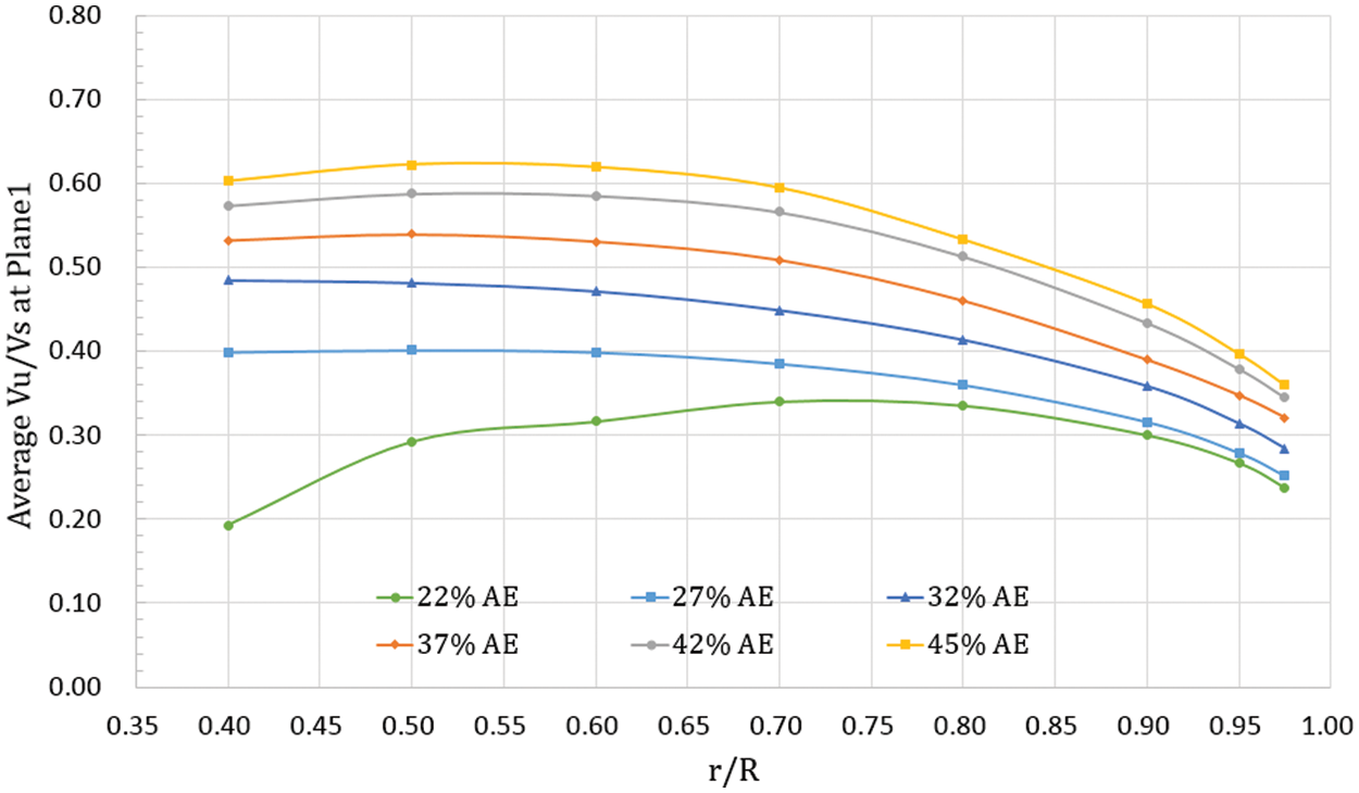
Figure 13: (1-W) distribution in different radial positions in Plane 1

6.2 Discussion at a Fixed Absorbed Horsepower

To be more consistent with the actual situation, in addition to the fixed ship speed and shaft rotational speed, this study examined the performance of nozzles under the scenario of using a fixed horsepower output. The rotor pitch ratio was adjusted to ensure consistent horsepower output. The rotor pitch ratio was adjusted based on the distribution of Rotor 27 in Fig. 9a. The distribution trend was fixed, but pitch ratios in all radial positions differed equidistantly.

Tables 7 to 11 present the pitch ratio adjustment results when nozzles with different outlet areas were used to make the torque absorbed by the rotor reach the target value (391.55 N-m). Fig. 14 shows the distribution of the pitch ratio of matched rotors after pitch ratio adjustments. To reduce the absorbed torque, at the 22%AE condition, the pitch ratio of Rotor 22–2 was reduced; at the 45%AE condition, due to the greatest horsepower loss, the pitch ratio of Rotor 45–2 was increased most significantly to reach the same absorbed horsepower as the 27%AE condition.

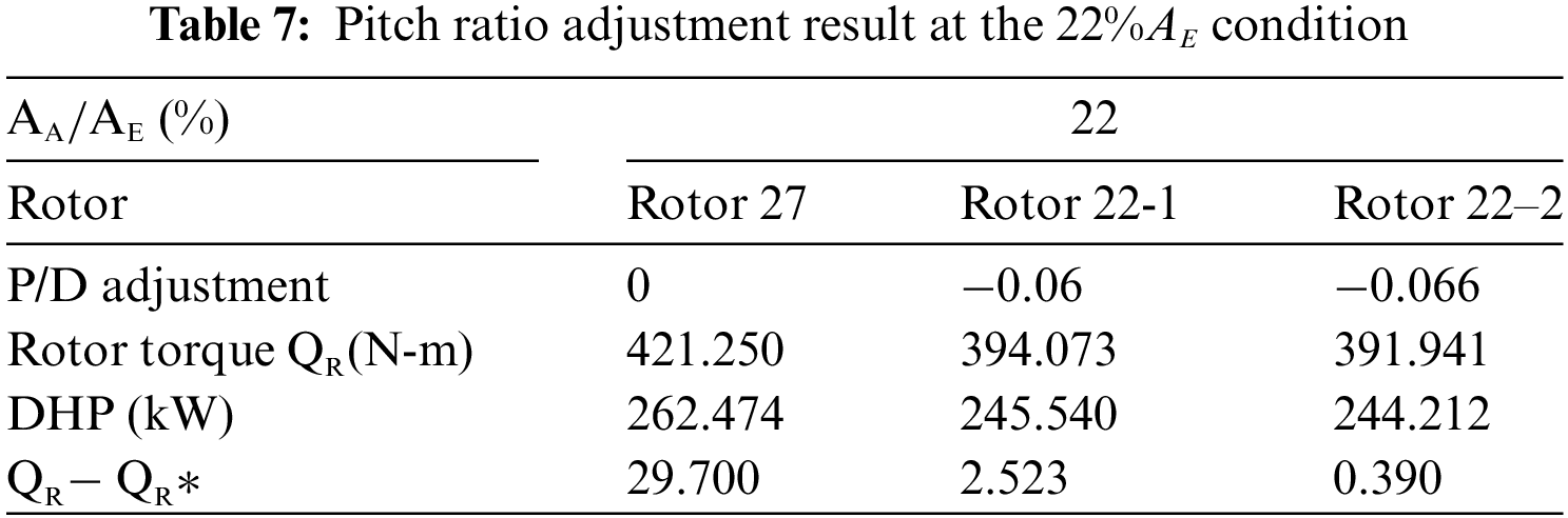
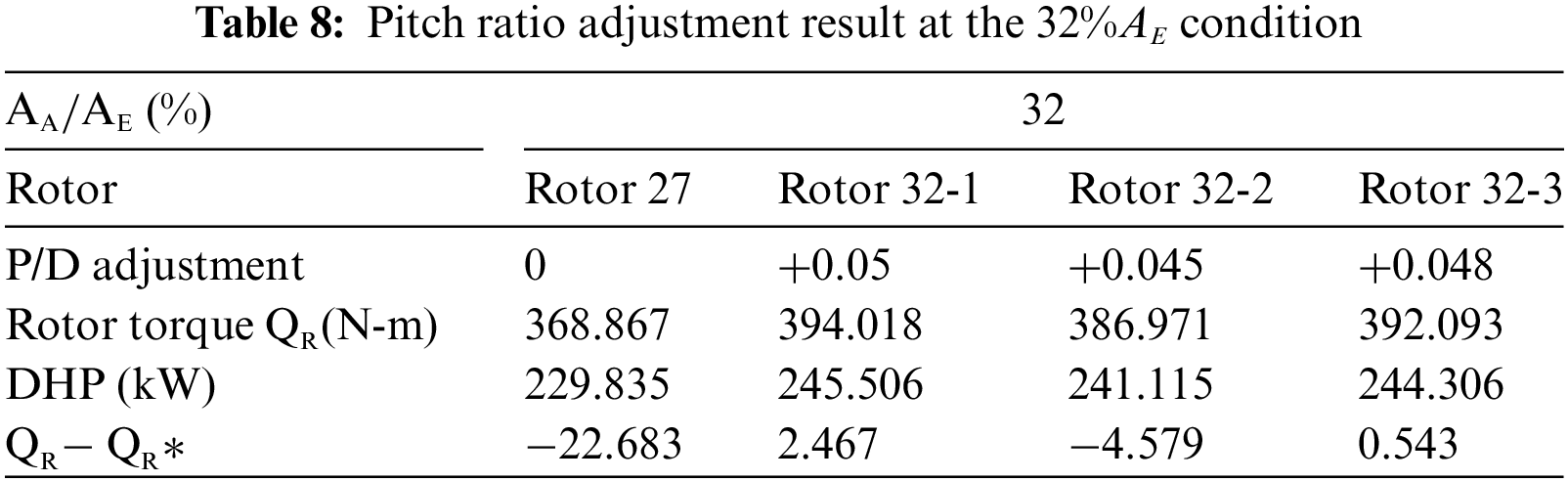
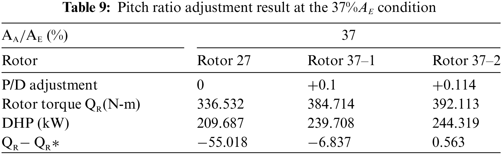
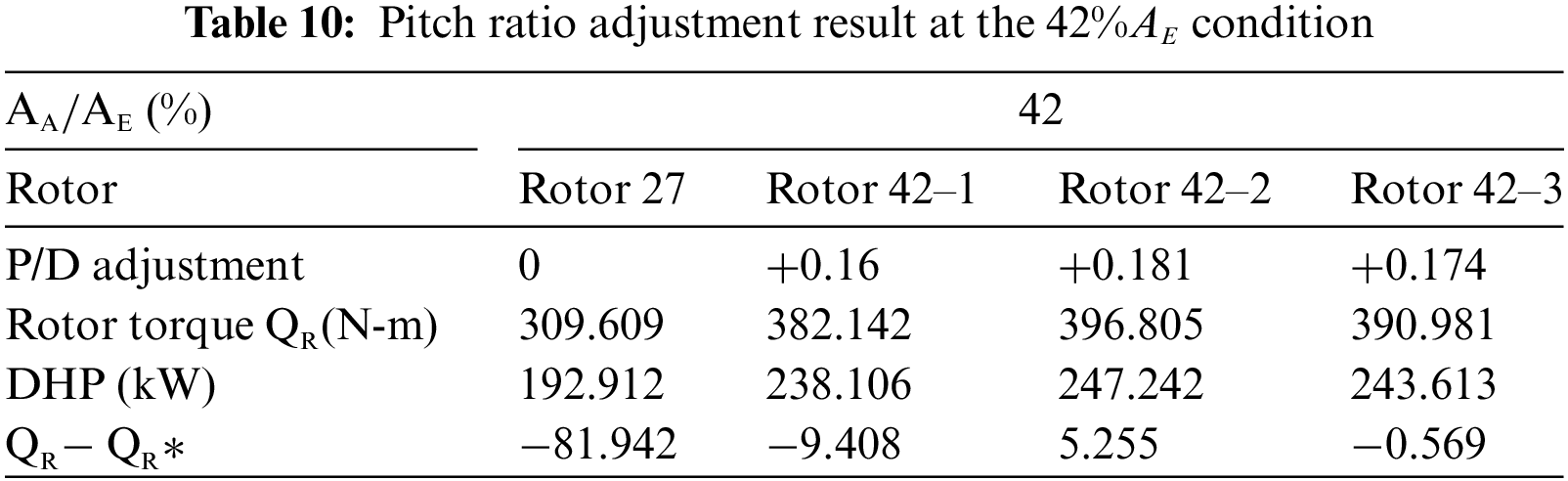
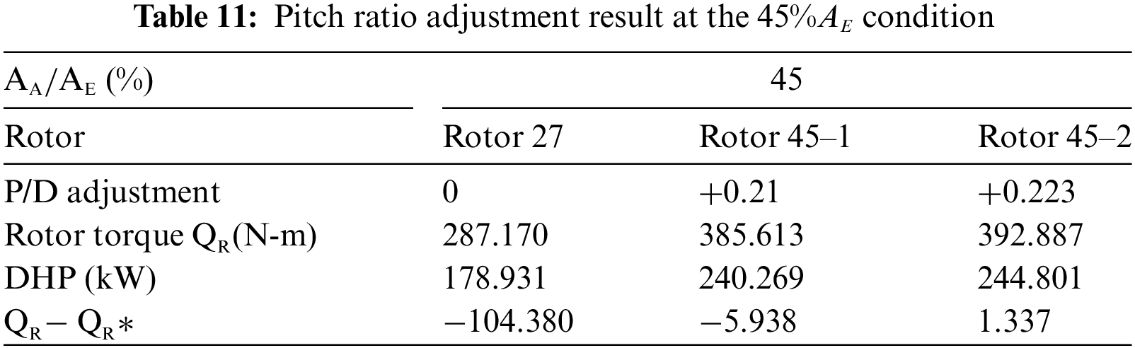
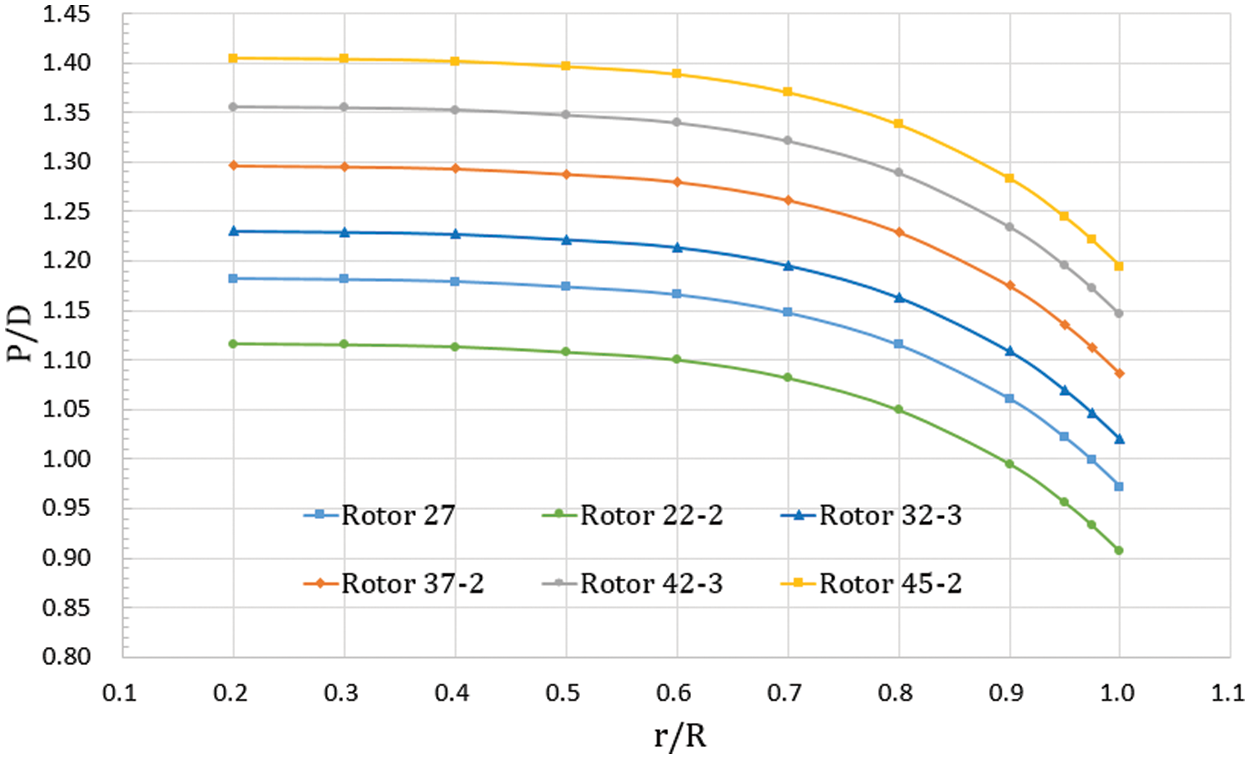
Figure 14: Distribution of pitch ratio of matched rotors at different outlet area conditions

Figs. 15 and 16 show the tendency of the rotor trust and flow rate at different outlet area conditions before and after the pitch ratio adjustment. The pitch increment could increase the net thrust and flow rate from the 32% to 45%AE conditions. At the 45%AE condition, net thrust increased most significantly due to the greatest increase in pitch ratio; as a result, fluid sucked by the intake increased most significantly. At the 22%AE condition, net thrust and flow rate decreased due to the decrease in pitch ratio. The net thrust and flow rate trend with outlet area remained unchanged before and after the pitch ratio adjustment. When the output area increased, the contribution of net thrust decreased. Fig. 17 shows the tendency chart of the head before and after the pitch ratio adjustment. After pitch ratio adjustment, when the output area increased, the contribution of the head decreased, which is in line with the net thrust trend. Taking the 45%AE condition as an example, after the pitch ratio adjustment, both net thrust and flow rate increased significantly. In particular, an increase in flow rate caused the dynamic pressure difference between Planes 1 and 2 to increase. Meanwhile, more increments in thrust caused the contribution of static pressure to increase. Therefore, the head coefficient increased most significantly under the combined effect of dynamic and static pressure (total pressure); however, the value was still the smallest among all computations.

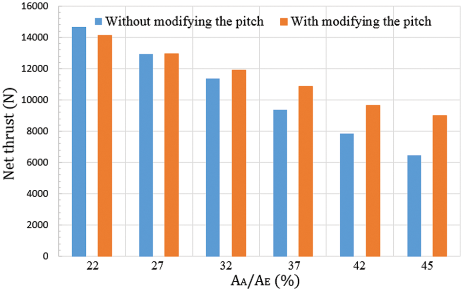
Figure 15: Tendency of the net trust at different outlet area conditions before and after the pitch ratio adjustment

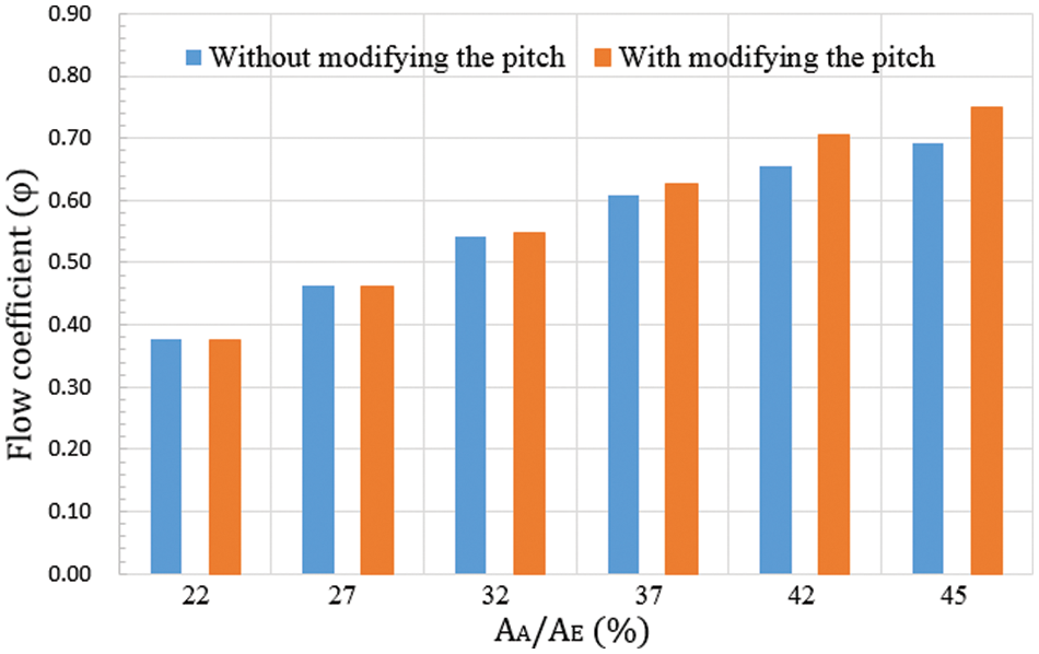
Figure 16: Tendency of the flow rate at different outlet area conditions before and after the pitch ratio adjustment

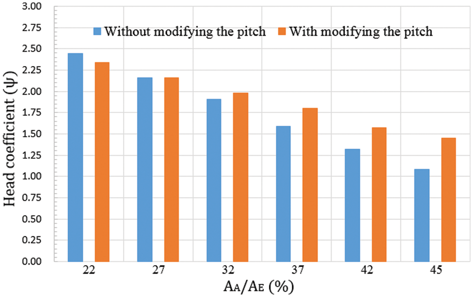
Figure 17: Tendency of the head coefficient at different outlet area conditions before and after the pitch ratio adjustment

Fig. 18 shows the comparison results of ultimate efficiency after pitch ratio adjustment at different outlet area conditions, including rotor and system efficiency. According to the computation results, both rotor and system efficiency decreased compared to those of the original design area at the 22%AE condition and increase at the 32% of AE condition. This trend suggests that it is not right to reduce the outlet area based on the 27%AE condition but increase the outlet area. As shown in Fig. 18 and according to the computation results listed in Table 12, 37%AE provided the highest efficiency of the system but a slightly lower efficiency of the rotor than that of 42%AE, which differed slightly. The pump efficiency should concurrently consider the head, flow, and shaft work, namely, the overall effect of the rotor, stator, and nozzle. However, the thrust efficiency only includes the impact of blade thrust (static pressure) and torque. Therefore, optimal pump efficiency is not equivalent to optimal thrust efficiency. Given the above, this study recommends the design outlet area be 37% to 42%AE. 37%AE provided the highest efficiency of the pump among all computations and represents a 9.8% increase over the original design area, indicating that at a fixed absorbed horsepower, using a nozzle with an outlet area of 37%AE can achieve an optimal balance between head and flow performance, i.e., the product of head and flow rate will be the greatest. Therefore, this study considers 37%AE as the optimal design of the nozzle outlet area.

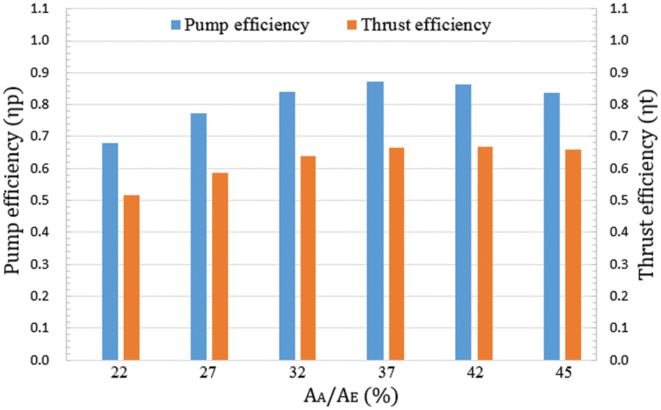
Figure 18: Relational graph of efficiency at different outlet area conditions

7  CFD Simulation Results of Different Nozzle Contours

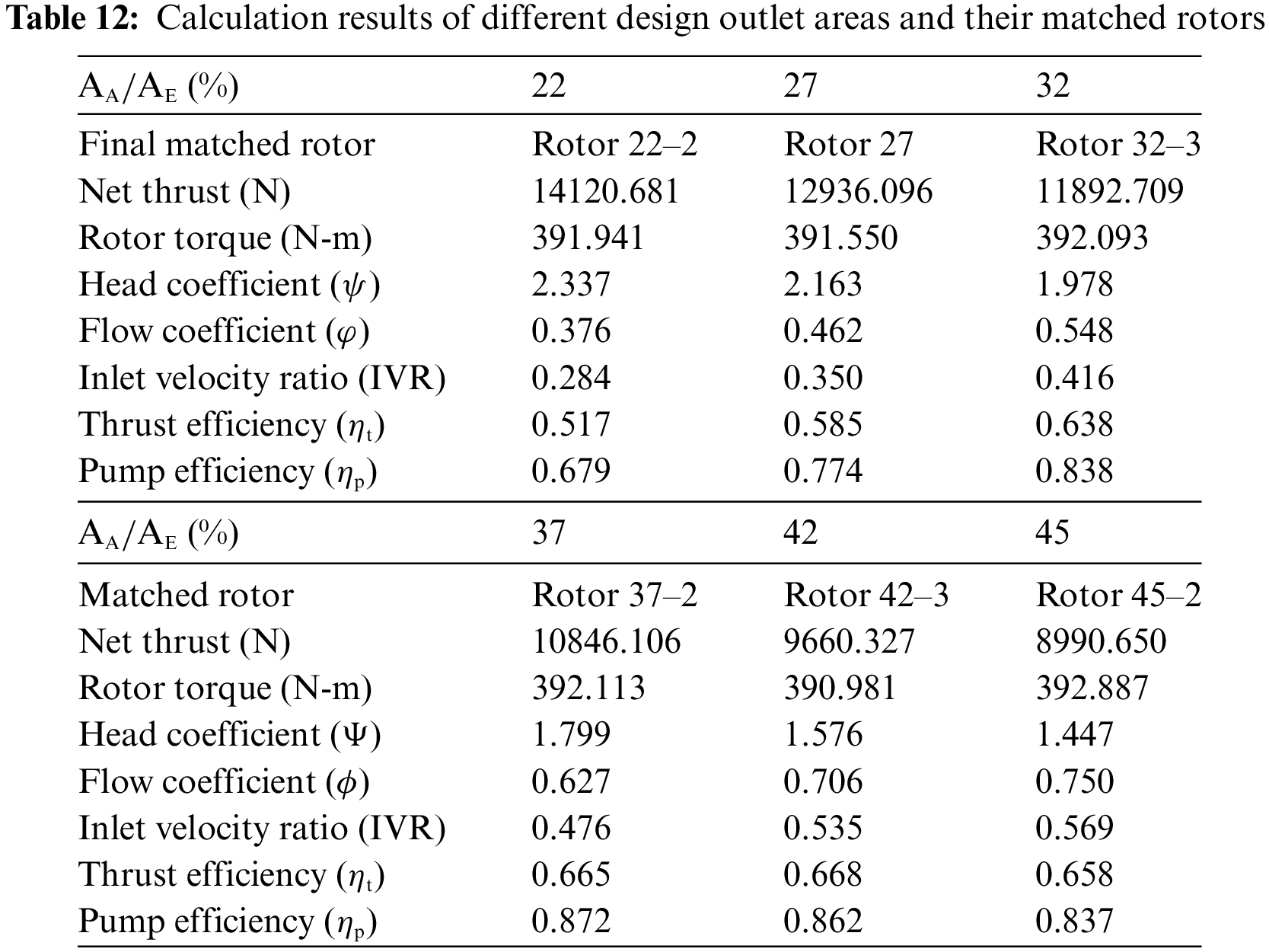
According to the simulation results of the linear nozzle contour with different outlet areas, 37%AE provided the highest system efficiency. In other words, at a fixed absorbed horsepower, 37%AE can help achieve an optimal balance between the head and the flow performance to the largest extent. We suggest the optimal design of the nozzle contour based on the optimization of different nozzle contours using 37%AE.

In addition to a linear nozzle shape, two nozzle contours with curvature changes were added. Therefore, a total of three nozzle contours were compared: Shapes A, B, and C. Table 13 lists the design parameters of these nozzle contours. Fig. 19 shows the geometric appearance of the three shapes. Shape A was a linear contraction form used uniformly for discussion in Section 3. Shapes B and C were obtained by rectifying the contour curvature. Shape C exhibited a greater curvature variation than Shape B (refer to Table 13).

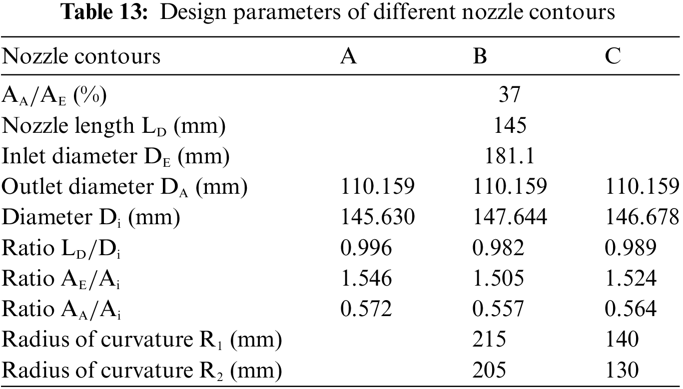
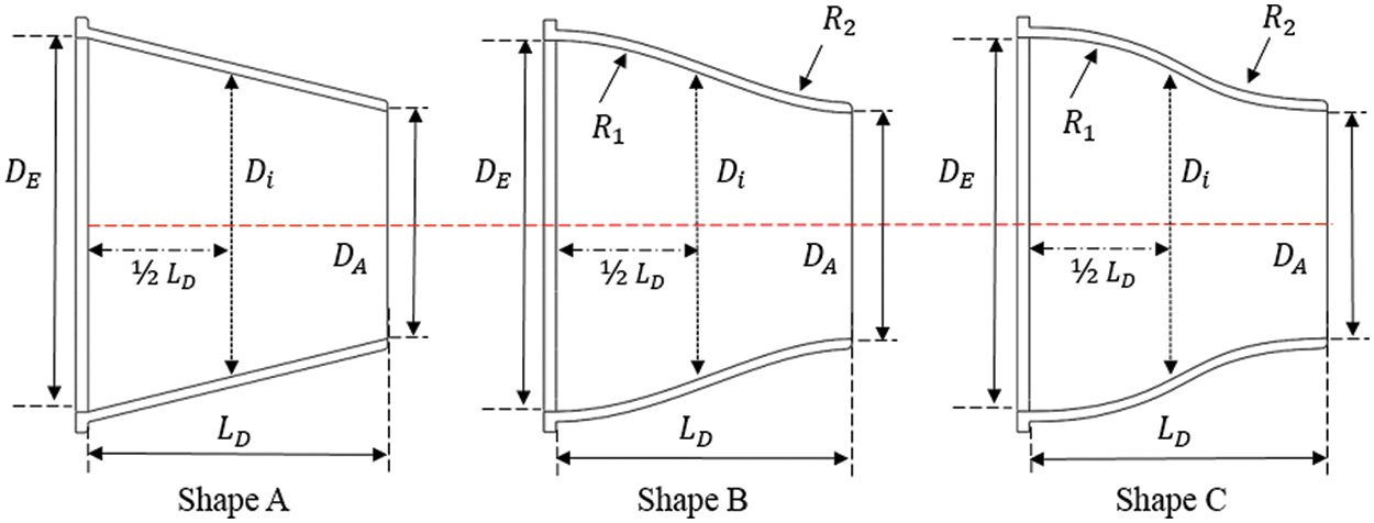
Figure 19: Geometric appearance of different nozzle contours

7.1 Qualitative Discussion

Table 14 lists the computation results when Rotor 27 was used with different nozzle contours. The flow rate at the Shapes B and C conditions was significantly higher than at Shape A. The flow rate at the Shape C condition was the highest. This indicates that with the same outlet area, a nozzle with a curved shape can lead to a more significant fluid acceleration effect so that intake velocity in front of the rotor and inlet velocity at the outlet both increase. Therefore, at the Shapes B and C conditions, the attack angle of the rotor inflow became smaller, so there was greater thrust loss and torque loss than in the Shape A condition. Fig. 20 shows the flow field’s static pressure distribution when Rotor 27 was used with different nozzle contours. The findings illustrate that the acceleration effect near the outlet at the Shapes B and C conditions was more significant than that at Shape A. Therefore, the static pressure at Shapes B and C was less than that at Shape A. At the Shapes B and C conditions, recovered low pressure at the nozzle outlet caused by fluid acceleration extended into the intake duct. This phenomenon was caused by the indenting trend at the tail of a curved shape, leading the sectional area to decrease, fluid to accelerate early, and pressure to drop. The indenting trend at the geometric tail of Shape C was the most significant. Therefore, the early acceleration and pressure decrease effects were the most significant. Additionally, there was significant thrust and torque loss at the Shapes B and C conditions. As shown in Fig. 20, there was no significant difference in pressure in front of or behind the rotor when Rotor 27 was used with Shapes B and C, compared to when Rotor 27 was used with Shape A. Fig. 21 shows the dynamic pressure distribution in the flow field when Rotor 27 was used with different shaped nozzles. At the Shapes B and C conditions, there was also significant early acceleration at the outlet, i.e., higher dynamic pressure extended from the outlet into the intake duct. In addition, as listed in Table 14, the head coefficient at the Shapes B and C conditions was lower than that at the Shape A condition. A more downward net thrust was provided at the Shapes B and C conditions so that the static pressure contributed less to the head coefficient. Furthermore, at the Shapes B and C conditions, early acceleration of fluid near the outlet increased the static pressure loss. The higher flow rate at the Shapes B and C conditions caused the dynamic pressure between Planes 1 and 2 to increase. However, the static pressure loss at the outlet was more significant than the dynamic pressure increase, further reducing the total head. Therefore, as listed in Table 14, the head coefficient at Shapes B and C conditions was lower than that at Shape A condition; in particular, the head coefficient at Shape C condition was the lowest.

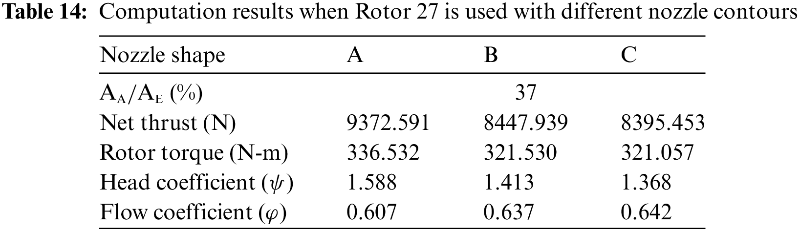
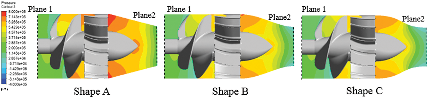
Figure 20: Distribution of static pressure in the flow field when using Rotor 27 with different nozzle contours

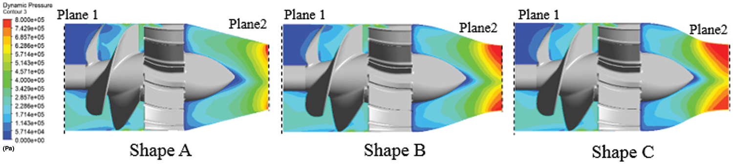
Figure 21: Distribution of dynamic pressure in the flow field when using Rotor 27 with different nozzle contours

7.2 Discussion at a Fixed Absorbed Horsepower

The rotor pitch ratio was adjusted in the same way as described in Section 3. Based on a fixed pitch distribution trend of Rotor 27, pitches in all radial positions differed equidistantly. Tables 15 to 17 list the pitch ratio adjustment results as the horsepower absorbed by the rotor reached the target value. Fig. 22 shows the distribution of the pitch ratio of rotors matching different nozzle shape conditions. The rotor pitch was significantly increased to reach the same torque and absorbed horsepower at the Shapes B and C conditions.

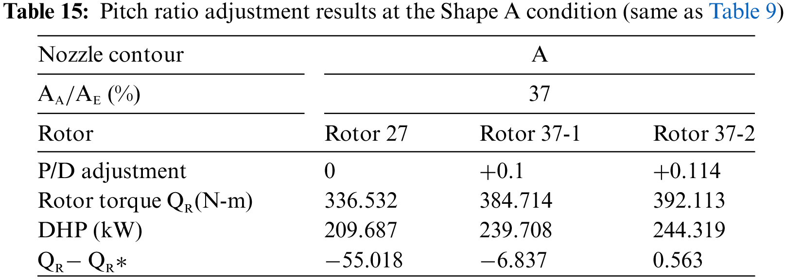
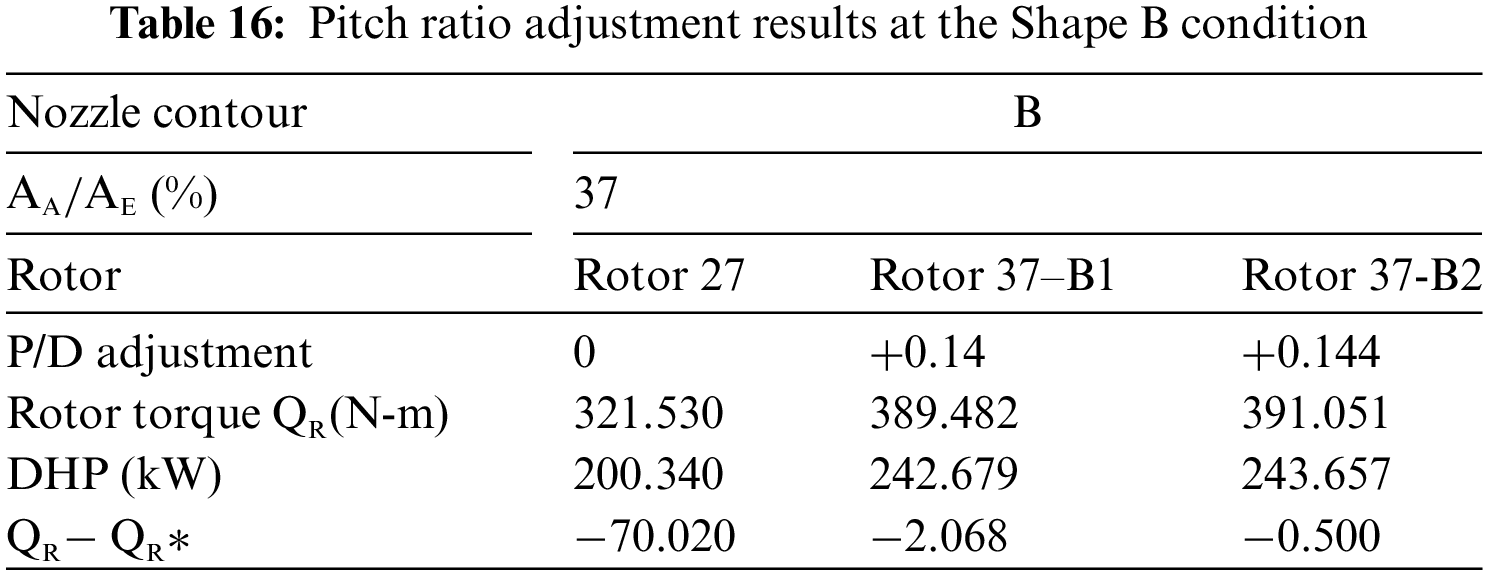
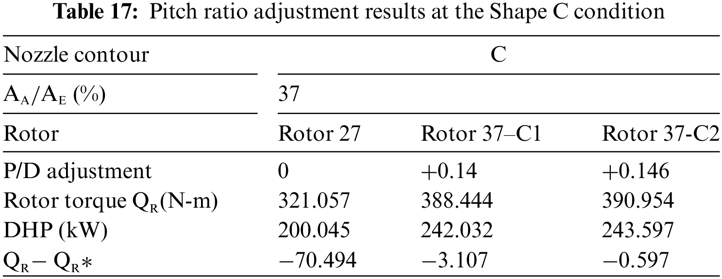
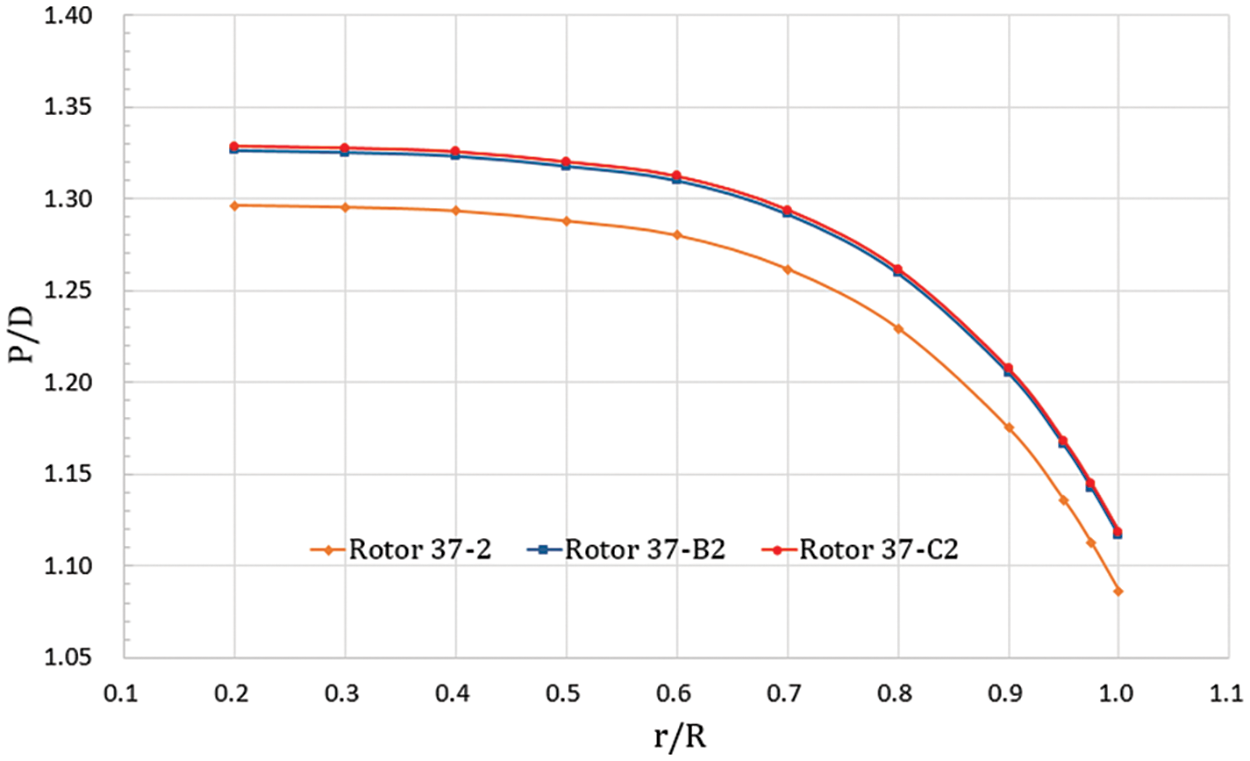
Figure 22: Distribution of pitch ratio of rotors matching different nozzle contour conditions

Table 18 lists the computation results of nozzles with different shapes used with matched rotor designs. Figs. 23 to 26 show the changes in net thrust, flow coefficient, head coefficient, and efficiency after rotor pitch adjustment.

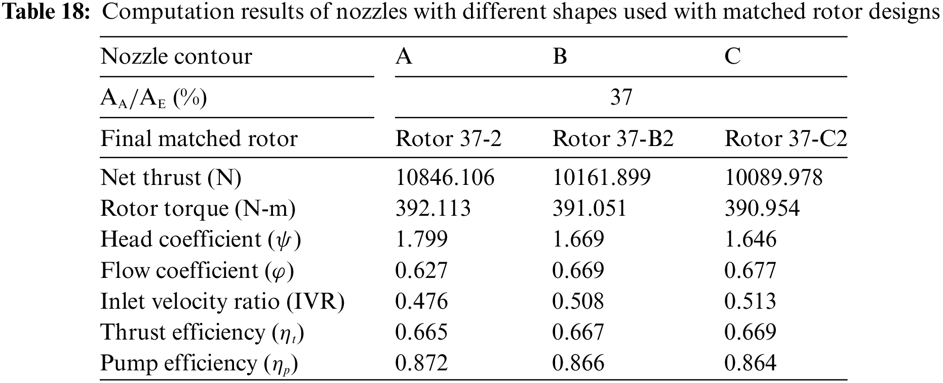
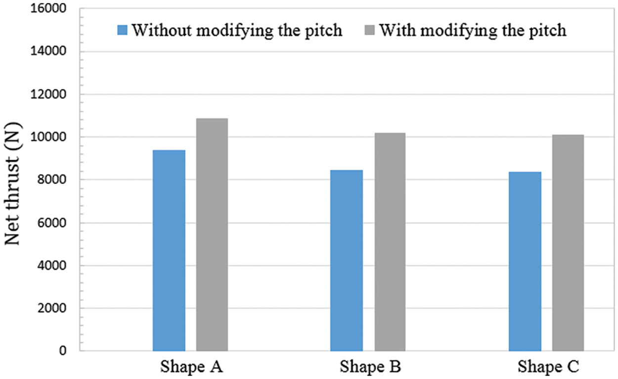
Figure 23: Tendency of the net thrust before and after the pitch ratio adjustment at different nozzle contour conditions

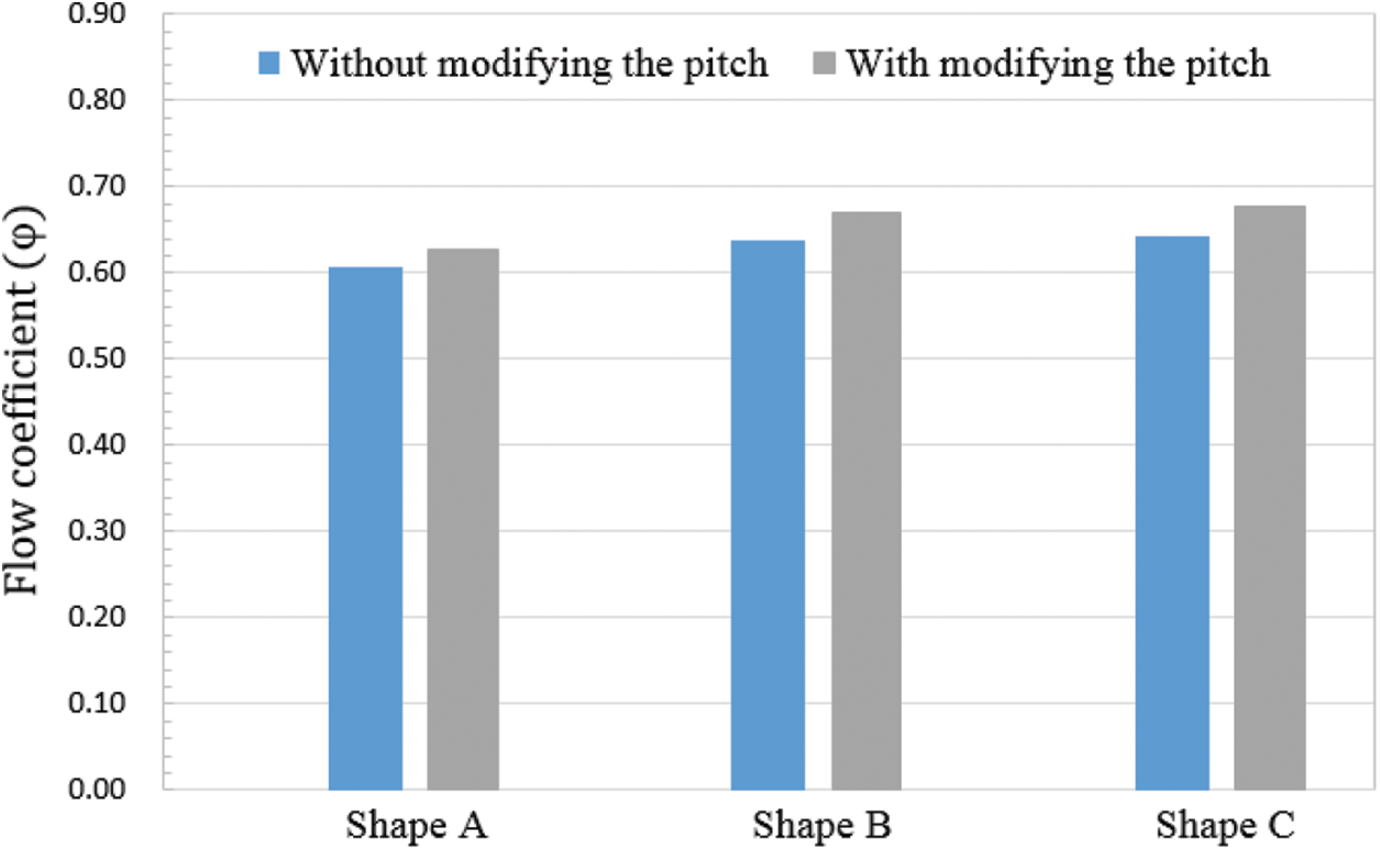
Figure 24: Tendency of the flow rate before and after the pitch ratio adjustment at different nozzle contour conditions

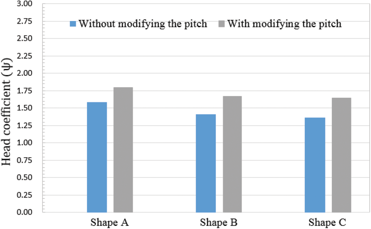
Figure 25: Tendency of the head before and after the pitch ratio adjustment at different nozzle contour conditions

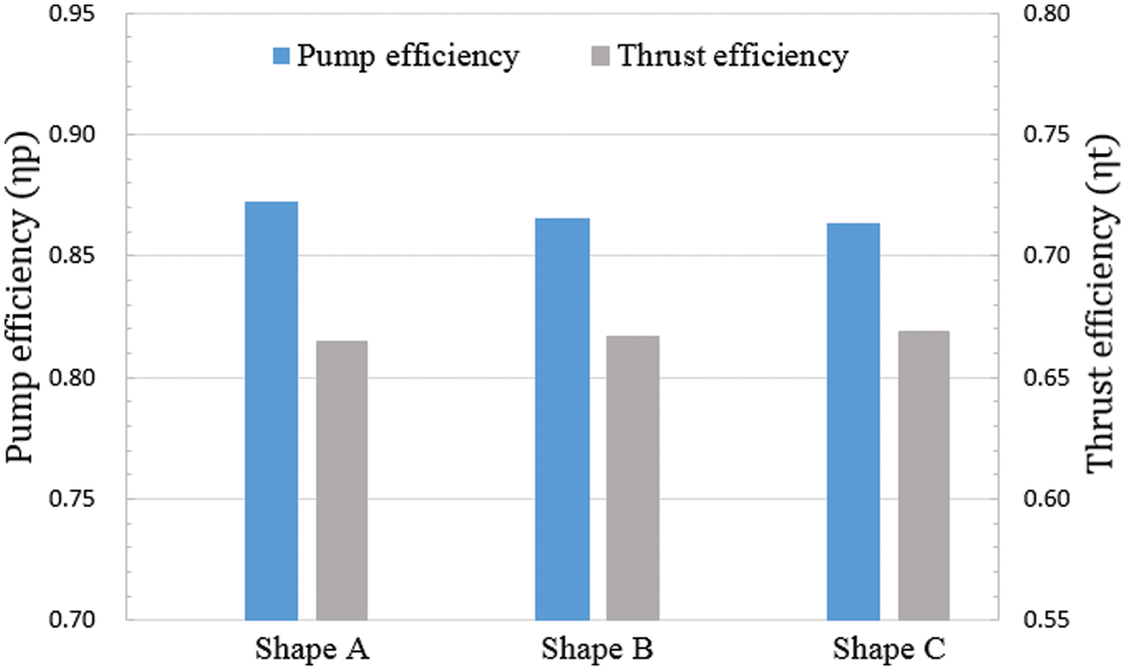
Figure 26: Relational graph of efficiency at different nozzle contour conditions

At the Shapes B and C conditions, there was a significant increase in pitch, which led to a higher net thrust and flow rate. At the Shape C condition, the highest increase in pitch resulted in the most significant increase in the net thrust and flow rate. The net thrust trend after the pitch adjustment was the same as that before the pitch adjustment. In other words, the Shapes B and C conditions provided a high flow rate and contributed less to the thrust than the Shape A condition. As shown in Fig. 25, at the same absorbed horsepower, the Shape C condition provided the most significant increase in the net thrust and flow rate. The increase in flow rate increased the dynamic pressure between Planes 1 and 2, while the increase in thrust also elevated the static pressure. Therefore, under the combined effect of dynamic and static pressure, the Shape C condition provided the most significant increase in the head coefficient. However, head performance after pitch adjustment at the Shapes B and C conditions was still inferior to that at Shape A. The primary cause was the same as described above: less net thrust contribution and early acceleration near the outlet cause static pressure loss.

Fig. 26 compares the efficiency in different nozzle contour conditions at the same absorbed horsepower. When the system used nozzles with different contours, the thrust efficiency varied slightly, possibly due to errors. Therefore, at the same absorbed horsepower, a nozzle shape change may not significantly impact the thrust efficiency. However, there was a slight difference in the pump efficiency compared to the thrust efficiency. The difference between the highest and lowest system efficiency was about 1.5%. As listed in Table 18, the linear shape, namely Shape A, delivered optimal pump efficiency. This indicates that at the same absorbed rotor horsepower, using a nozzle with this shape helped achieve an optimal balance between the head and the flow performance. Hence, Shape A was the optimal nozzle contour in this study. This finding is consistent with Wang et al. [11], who found the optimal efficiency of a pump using a linear taper-shaped nozzle. As discussed above, nozzles with a curved shape can increase the flow rate but lower the head performance. This is possibly due to the more apparent static pressure loss at the outlet than dynamic pressure increases so that the head was reduced to diminish the pump efficiency. Therefore, as listed in Table 18, the pump efficiency at the Shapes B and C conditions was inferior to that at Shape A due to more significant head loss than flow increase. This study recommends the linear nozzle shape, namely Shape A.

8  Conclusions

This study simulated the performance and optimized the design of an existing water jet propulsion pump system by CFD. A jet ski geometry model and free surface were considered in the computational domain to make the inflow in the water duct more approximate to the actual situation. The following conclusions are drawn based on the CFD simulation results:

1.    This study discussed the impacts of the nozzle outlet area and shape on the system’s performance. During the comparison, this study adjusted the rotor pitch to ensure consistent horsepower absorbed by the system. Discussion on performance based on the same absorbed horsepower better conforms to the actual situation.

2.    This study computed the head based on total pressure. That is, this study computed the total head under the combined effect of the rotor, stator, and nozzle. The total head includes a static and dynamic head. The former is affected by the thrust generated by the stator and rotor, and the latter is the effect provided by the gradually contracting shape of the nozzle.

3.    This study recommends 37%AE for the optimal design, as it could increase the system efficiency by 9.8%.

4.    The linear nozzle contour delivers the optimal pump efficiency. This finding is consistent with Wang et al. [11]. Moreover, curved nozzles can increase the fluid’s acceleration effect, meaning a higher flow rate, but they do not improve head performance. The static pressure loss at the outlet was more significant than the dynamic pressure increase, which further reduces the head and diminishes the system’s efficiency.

Acknowledgement: We extend our gratitude to Dr. Young-Zehr Kehr (Professor Emeritus, National Taiwan Ocean University) for providing the useful comments on this study.

Funding Statement: The author (Jui Hsiang Kao) wishes to thank the financial support from the National Science and Technology Council, Taiwan (Grant No. MOST 111-2221-E-019-035-).

Author Contributions: The authors confirm contribution to the paper as follows: study conception and design: Cheng-Yeh Li, Jui-Hsiang Kao; data collection: Cheng-Yeh Li; analysis and interpretation of results: Cheng-Yeh Li, Jui-Hsiang Kao; draft manuscript preparation: Cheng-Yeh Li, Jui-Hsiang Kao. All authors reviewed the results and approved the final version of the manuscript.

Availability of Data and Materials: The authors confirm that the data supporting the findings of this study are available within the article. Raw data that support the findings of this study are available from the corresponding auther, upon reasonable request.

Conflicts of Interest: The authors declare that they have no conflicts of interest to report regarding the present study.

References

1. Jung, K. H., Kim, K. C., Yoon, S. Y., Kwon, S. H., Chun, H. H. et al. (2006). Investigation of turbulent flows in a waterjet intake duct using stereoscopic PIV measurements. Journal of Marine Science and Technology, 11, 270–278. [Google Scholar]

2. Eslamdoost, A., Larsson, L., Bensow, R. (2018). Analysis of the thrust deduction in waterjet propulsion—the froude number dependence. Ocean Engineering, 152, 100–112. [Google Scholar]

3. Brandner, P. A., Walker, G. J. (2019). An experimental investigation into the performance of a flush water-jet inlet. Journal of Ship Research, 51(1), 1–21. [Google Scholar]

4. Timur, D., Hamid, S. H., Frederick, S. (2022). Effects of hook, interceptor, and water jets on LCS resistance/power, sinkage, and trim. Journal of Ship Research, 66(2), 127–150. [Google Scholar]

5. Wang, P., Shi, D. Y., Cui, X. W., Su, B., Li, G. et al. (2023). Study on the physical mechanism of water layer on the morphological evolution of transient-pulse high-speed water jet. Ocean Engineering, 267, 113–238. [Google Scholar]

6. Jiao, W. X., Zhao, H., Cheng, L., Yang, Y., Li, Z. et al. (2023). Nonlinear dynamic characteristics of suction-vortex-induced pressure fluctuations based on chaos theory for a water jet pump unit. Ocean Engineering, 268, 113–429. [Google Scholar]

7. Lu, L., Pan, G., Sahoo, P. K. (2016). CFD prediction and simulation of a pumpjet propulsor. Ocean Engineering, 8, 110–116. [Google Scholar]

8. Park, W. G., Yun, H. S., Chun, H. H., Kim, M. C. (2005). Numerical flow simulation of flush type intake duct of waterjet. Ocean Engineering, 32(17–18), 2107–2120. [Google Scholar]

9. Gao, H., Lin, W., Du, Z. (2008). Numerical flow and performance analysis of a water-jet axial flow pump. Ocean Engineering, 35(16), 1604–1614. [Google Scholar]

10. Hu, F. F., Wu, P., Wu, D. Z., Wang, L. Q. (2014). Numerical study on the stall behavior of a water jet mixed-flow pump. Journal of Marine Science and Technology, 19, 438–449. [Google Scholar]

11. Wang, C., He, X., Cheng, L., Luo, C., Xu, J. et al. (2019). Numerical simulation on hydraulic characteristics of nozzle in waterjet propulsion system. Processes, 7(12), 915. https://doi.org/10.3390/pr7120915 [Google Scholar] [CrossRef]

12. Wu, J., Cheng, L., Luo, C., Wang, C. (2021). Influence of external jet on hydraulic performance and flow field characteristics of water jet propulsion pump device. Shock and Vibration, 2021, 6690910. https://doi.org/10.1155/2021/6690910 [Google Scholar] [CrossRef]

13. Chen, X., Cheng, L., Wang, C., Luo, C. (2021). Influence of inlet duct length on the hydraulic performance of the waterjet propulsion device. Shock and Vibration, 2021, 6676601. https://doi.org/10.1155/2021/6676601 [Google Scholar] [CrossRef]

14. Jiao, W., Cheng, L., Zhang, D., Zhang, B., Su, Y. et al. (2019). Optimal design of inlet passage for waterjet propulsion system based on flow and geometric parameters. Advances in Materials Science and Engineering, 2019, 2320981. https://doi.org/10.1155/2019/2320981 [Google Scholar] [CrossRef]