A Combustion Model for Explosive Charge Affected by a Bottom Gap in the Launch Environment

1  Introduction

Launch safety is one of the basic requirements for weapon performance. As the need for continual improvement in weapon performance increases, the launch situation for ammunition becomes consistently worse, and the phenomenon of bore burst has become a bottleneck restricting high–performance weapon development [1]. In the case of a 175 mm American artillery loaded with Composition B (COM B) explosive charge, the bore burst rate is reportedly as high as 0.04% [2], resulting in serious weapon destruction and casualties. The accidental ignition of explosive charges in the launch environment is one of the primary reasons for bore bursts, the mechanism of which has been the focus of considerable research on the launch safety of explosive charges [3,4]. Many scholars [5–10] have examined the stress, action time, and hot–spot generation of an explosive charge in the launch environment, finding that factors influencing accidental ignition are the particle size, pores, bottom gaps, cracks, and other defects associated with the explosive charge [11–15]. Wu et al. [11] analyzed the influence of particle size on the ignition process and showed that the ignition time increases monotonically with decreasing particle size (50–200 μm). By simulating the compression of the pore space inside an explosive charge under a launching load, Li et al. [12] found that the pore volume change is a major factor affecting the formation of ignition hot spots. Zhang et al. [16] reported that pores with a diameter of less than 0.3 mm have a negligible effect on the sensitivity of a COM B explosive charge under the impact of a drop weight. Based on two–phase flow theory, Liu et al. [1] studied the effect of the initial porosity on the ignition of an explosive charge in the launch environment, with the results showing that the initial porosity of explosives should be strictly controlled below 0.8 to ensure launch safety. Zhou et al. [17] used a self–built stress–test device and showed that, during the launch process, the air trapped in the bottom gap below the explosives is adiabatically compressed under recoil impact, thus raising the temperature of the explosive surface adjacent to the air and increasing the likelihood of a high–temperature hot spot forming. They [18] found that the ignition threshold of an explosive charge increases significantly as the bottom gap decreases, and so the thickness of this gap should be controlled to within the smallest possible range. The U.S. Army Ballistic Research Institute [19] studied the shear deformation ignition mechanism of COM B explosive charge with prefabricated defects using a BRL exciter, and found that the bottom gap of the explosive charges is particularly sensitive to the response of a firing overload. Yu et al. [20] pointed out that the explosive bottom temperature continues to increase until the explosives ignites, i.e., once the air in the bottom gap has been compressed to a certain extent. Qiang et al. [21] used a numerical model of the small–scale gap test to obtain the critical gas thickness for the detonation reaction of a solid propellant. Cheng et al. [22] simulated the detonation process of explosive trains with a micro–sized air gap and concluded that the critical air gap thickness ranges from 0.32–0.40 mm. Following a series of underwater experiments, Xiao et al. [23] concluded that COM B explosive charge can explode and has a peak pressure of 1600 MPa during launch with a bottom gap of 0.38 mm. Using the finite element method to simulate the stress distribution of explosives affected by the bottom gap in the firing process, Li et al. [2] reported that the bottom gap should be less than 0.5 mm to prevent the explosive charge from exploding during the firing process. The U.S. Naval Weapons Laboratory found that the maximum bottom gap for a COM B explosive charge should not exceed 0.381 mm to ensure launch safety under a simulated pressure of 506 MPa [24]. Meng et al. [25] determined a reasonable method of eliminating the bottom gap of explosive charges using a custom pressure sensor, while Yang et al. [26] proposed an ultrasonic inspection method that can effectively detect the bottom gap based on the conservation of sound flux in propagation. This series of research reports on the impact of the bottom gap on explosive charge safety in the launch environment has verified that the bottom gap is one of the main reasons for explosive charge blowout. However, explosive charge safety in the presence of a bottom gap has generally been studied under unconstrained conditions (such as with no cartridge), and the relation between the bottom gap thickness and the explosive temperature has not been considered in previous researches. At the same time, the existing numerical models have different defects, such as low computational efficiency and processing convection terms, which seriously affects the accuracy of results.

The material point method (MPM) is a meshless approach developed from the fluid–implicit–particle method [27]. The MPM adopts the dual description of a Lagrangian particle and an Eulerian grid, combining the advantages of Lagrangian and Eulerian methods [28,29]. It eliminates the numerical difficulties arising from grid distortion and nonlinear convection terms [30–34]. As the Lagrangian particle mass does not change in the calculation process, the mass conservation condition is always satisfied in the MPM. Simultaneously, the Lagrangian particle motion variables are updated by mapping the results of the motion equations onto the grid nodes, which satisfies the non–slip condition in the MPM. Several scholars have also developed other meshless methods to solve mechanical problems, such as the cracking particles method [35,36] and the reproducing kernel particle method [37] for describing dynamic crack propagation, the peridynamics-SPH method [38–40] for simulating the explosive fragmentation of soil, the deep energy method [41] for avoiding discretization, the nonlocal operator method [42,43] for solving partial differential equations of mechanical problems, the dual–horizon peridynamics method [44] for solving the problem of stray wave reflection with a variable horizon, the localized Fourier collocation method [45] for solving numerically large-scale boundary value problems with complex-shape geometries, the fluid–structure interaction [46] for investigating the problems of fluid–structure interaction, and the coupled model [47] for researching the buffer performance of the thin-walled circular tube in the launch safety problems. Compared to other meshless methods, the MPM has higher computational efficiency and accuracy, better tension stability, and can easily deal with material breakage and fluid–structure interactions [48–50]. During the launch process of an explosive charge affected by a bottom gap, the volume of gas in the bottom gap and generated by the combustion of developed can change greatly, and fluid–structure coupling can occur between the gas and the solid. Therefore, the MPM is selected in this study.

In this paper, a combustion model is developed using the thermal equilibrium equation, viscoelastic statistical crack mechanics (Visco–SCRAM) model, and a virial equation. Using this model, we study the safety of an explosive charge in the presence of a bottom gap under constrained conditions in the launch environment. The effect of microcracks on the explosive temperature under the action pressure is also considered. Subsequently, the relationship between the bottom gap thickness and explosive temperature in the launch environment is investigated. Ultimately, the critical thickness of the explosive bottom gap in the launch environment is determined. The model developed in this paper is the first application of the MPM in the study of launch dynamics. Thus, this study extends the application field of the MPM and provides a method for examining the launch safety of explosive charges.

2  Material Point Method

The MPM contains Lagrangian particles and an Eulerian grid, as shown in Fig. 1. A continuous material is separated into a series of Lagrangian particles in the MPM. Physical variables (including mass, momentum, temperature, stress, etc.) associated with the material are stored in the Lagrangian particles. These particles characterize the motion and deformation state of the material region, thus avoiding the convection term problem. The background grid of the region in which the material is located is described by the Eulerian method. The physical variables of the Lagrangian particles are mapped to the background grids, the motion equations and the heat conduction terms of heat balance equations are solved on the grid nodes, and then the physical variables of the grids are mapped back to the Lagrangian particles. The physical variables of the Lagrangian particles are then updated. The thermal effect term caused by chemical decomposition term, plastic work term, and crack friction term of the heat balance equation are calculated in the Lagrangian particles, and are superimposed with the temperature of the Lagrangian particles to obtain the final temperature of the Lagrangian particles at the current time step.

Figure 1: Discrete schematic diagram of MPM

The material must satisfy the conservation of mass, momentum and energy in the MPM. The conservation equations of mass and momentum are, respectively

dρdt+ρ∇⋅v=0(1)

ρdvdt=∇⋅σ+ρb(2)

In this paper, the derivation of the energy equation is performed while neglects the heat exchange and heat source. Consequently, the rate of change of the total system energy is balanced by the power of the external force acting on the system.

ρdedt=σ:dεdt(3)

where ρ=ρ(x,t) is the particle density, v=v(x,t) is the velocity vector, ∇ is the divergence operator of a vector function, ∇⋅v=∂vi∂xi is the divergence of the velocity vector, σ=σ(x,t) is the Cauchy stress tensor, b=b(x,t) is the body force per unit mass, e is the energy per unit mass, ε=ε(x,t) is the strain tensor, and dεdt is the strain rate tensor.

The MPM calculation process in a single time step is as follows. In this description, i and p are the node number and particle number, respectively, and t is the time. The mass and momentum of the grid nodes are solved by mapping the mass and momentum of the particles.

Mass equation:

mit=∑p=1npmpNi,pt(4)

Momentum equation:

pit=∑p=1npmpvptNi,pt(5)

where pit and vpt are the momentum of node i and the velocity of particle p at time t, respectively, Ni,pt is the shape function, and mit, mp denote the mass of node i and particle p, respectively.

The internal force fiint,t of the nodes is

fiint,t=−∑p=1npmpρptσpt⋅∇Ni,pt(6)

and the external force fiext,t of the nodes is

fiext,t=∑p=1NpmpNi,ptbpt+∫Γττ¯ptNi,ptds(7)

where ρpt, σpt and bpt are the density, stress tensor and body force of particle p at time t, respectively, Γτ is the traction boundary, and τ¯pt is the surface traction.

The shape function Ni,pt of the generalized interpolation MPM is

Ni,pt=Ni,p,xt×Ni,p,yt(8)

where Ni,p,jt(j=x,y) is the component at the j direction and can be expressed as

Ni,p,jt={0|xp,j−xi,j|≥Lj+lp,j(Lj+lp,j+(xp,j−xi,j))24Ljlp,j−Lj−lp,j<xp,j−xi,j≤−Lj+lp,j1+xp,j−xi,jLj−Lj+lp,j<xp,j−xi,j≤−lp,j1−(xp,j−xi,j)2+lp,j2Lj−lp,j<xp,j−xi,j≤lp,j1−xp,j−xi,jLjlp,j<xp,j−xi,j≤Lj−lp,j(Lj+lp,j−(xp,j−xi,j))24Ljlp,jLj−lp,j<xp,j−xi,j≤Lj+lp,j(9)

where Lj is the mesh size in j direction, lp,j is the characteristic length of particle p in j direction, and xp,j, xi,j are the coordinates of particle p and node i in j direction, respectively.

The derivative ∇Ni,p,jt(j=x,y) of the shape function is

∇Ni,p,jt={0|xp,j−xi,j|≥Lj+lp,jLj+lp,j+(xp,j−xi,j)2Ljlp,jNi,p,j¯t−Lj−lp,j<xp,j−xi,j≤−Lj+lp,j1LjNi,p,j¯t−Lj+lp,j<xp,j−xi,j≤−lp,j−xp,j−xi,jLjlp,jNi,p,j¯t−lp,j<xp,j−xi,j≤lp,j−1LjNi,p,j¯tlp,j<xp,j−xi,j≤Lj−lp,j−Lj+lp,j−(xp,j−xi,j)2Ljlp,jNi,p,j¯tLj−lp,j<xp,j−xi,j≤Lj+lp,j(10)

where j¯ is determined based on j and j¯={x j=yy j=x

The momentum of the grid nodes can be calculated in terms of the internal force and the external force.

pit+1=pit+(fiint,t+fiext,t)Δt(11)

where pit+1 is the momentum of node i, and Δt is the time step.

The velocity vpt+1 and position xpt+1 of the particles are updated by mapping the momentum and force of the grid nodes to the particles.

vpt+1=vpt+∑i=1ni(fiint,t+fiext,t)mitNi,ptΔt(12)

xpt+1=xpt+∑i=1nipit+1mitNi,ptΔt(13)

The strain increment of the particles is obtained from the node velocity. Finally, the density ρpt+1 and characteristic length lpjt+1 of the particles are calculated by

ρpt+1=ρpt1+Δεxx+Δεyy+Δεzz(14)

lpjt+1=lpjt(1+Δεjj)(j=x,y,z)(15)

where Δεjj is the strain increment and j is the coordinate direction.

After those steps, the background grid is restored to the original state to prevent the distorted grid from being used in the next time step. The MPM calculation process is illustrated in Fig. 2.

Figure 2: Single time–step process of the MPM

3  Simulation Methodology

To study on the effect of the bottom gap on an artillery loaded with the COM B explosive charge in the launch environment, a combustion model is developed. A physical schematic diagram of the artillery is shown in Fig. 3. The physical objects within the model embody steel, explosive charge and air in the bottom gap. The constitutive model, state equation and heat balance equation of the objects are introduced in the following content.

Figure 3: Schematic diagram of the physical model

3.1 Mathematical Model of Steel

3.1.1 Constitutive Model of Steel

The Johnson–Cook plasticity model [51,52] provides a powerful description of the work–hardening, strain–rate, and temperature–softening effects of metals. This model is mainly applied to plastic metalworking, large deformation, and ballistic intrusion impact dynamics problems. Therefore, the von Mises flow stress σy is calculated by the Johnson–Cook model in this study:

σy=(A+Bεpn)(1+Cln⁡ε¯p∗)(1−T∗m)(16)

where A, B, C, n, and m are material constant, with B and n representing the strain-hardening characteristic of materials, C representing the strain rate–sensitive characteristic of materials, m representing the strain softening characteristic of materials, εp and ε¯p∗ denoting the equivalent plastic strain and equivalent plastic strain rate, respectively, and the homologous temperature T∗ calculated from the melting temperature Tmelt and room temperature Troom according to

T∗=T−TroomTmelt−Troom(17)

where T is the material temperature. The material parameters are listed in Table 1 [53].

3.1.2 Equations of State (EOS) of Steel

The shock equation is a special form of the Mie–Grüneisen equation, and is expressed as

p=pH+Γρ(e−eH)(18)

pH=ρ0c02μ(1+μ)[1−(1−s)μ]2(19)

eH=12pHρ0(μ1+μ)(20)

where ρ and ρ0 represent the current and original density, respectively, c0 is the sound speed at p = 0, s is a material parameters, Γ is the Grüneisen coefficient, and μ is the compression degree. The material parameters are listed in Table 2 [54].

3.2 Mathematical Model of Air

3.2.1 EOS of Air

The residual gas (air) in the bottom gap can be considered as an ideal gas in the numerical simulation. The EOS of an ideal gas [55] is indicated as

paVa=nRTa(21)

where pa, Va, Ta and n denote the pressure, volume, temperature and the amount of substance, respectively, and R is a constant.

3.2.2 Temperature Calculation of Air

This paper assumes that the process of air compression is adiabatic in a single time step. Therefore, the ideal gas quasi–static adiabatic equation is used to describe the air state. This equation can be expressed as follows:

paVaγ=C(22)

where pa and Va are the pressure and volume of the ideal gas, separately, γ is the ratio of constant pressure heat capacity ca,p to constant body heat capacity ca,V (approximately 1.4 in an ideal gas), and C is a constant.

From Eqs. (22) and (21), we can derive

paVaγ1−γ=C1(23)

TaVaγ−1=C2(24)

where C1 and C2 are constants. From Eqs. (23) and (24), we can deduce that

Ta,2=Ta,1(pa,2pa,1)γ−1γ=Ta,1εγ−1γ(25)

Ta,2=Ta,1(Va,1Va,2)γ−1=Ta,1εγ−1γ(26)

ε=pa,2pa,1=(Va,1Va,2)1γ(27)

where Ta,1, pa,1 and Va,1 respectively are temperature, pressure, and volume of ideal gas at the initial time, Ta,2, pa,2 and Va,2 respectively are temperature, pressure, and volume of ideal gas at the current time. From Eqs. (25) and (26), when Ta,1 is a constant, Ta,2 is only related to the compression ratio ε defined by Eq. (27).

Fig. 4 shows the air temperature at different compression ratios for Ta,1 = 300 K. When the compression ratio ε = 1.5, Ta,2 = 337 K. When ε = 3.0, Ta,2 rises to 413 K, when ε is 9.5, Ta,2 reaches 571 K. Thus, a higher compression ratio ε produces a higher temperature Ta,2.

Figure 4: The air temperature crave at different compression ratios

3.3 Mathematical Model of Explosive Charge

3.3.1 Constitutive Model of Explosive Charge

The viscoelastic statistical crack mechanics (Visco–SCRAM) model successfully combines the macroscale behavior of materials and the micro–crack behavior to simulate complex mechanical–thermal–chemical processes [56]. The model describes the mechanism of microcrack extension, coupling the microcrack body with the viscoelastic body [55,57,58], and reflects the viscoelastic mechanical properties and damage process of explosives, thus providing a realistic reflection of the mechanical properties of explosives [59,60]. Therefore, the Visco–SCRAM model is applied to describe the mechanical properties of explosive charge in this study. The model is composed of a generalized viscoelastic body and a microcrack body, as shown in Fig. 5. The generalized viscoelastic body is a parallel combination of multiple Maxwell bodies containing a viscous element and an elastic element, and the microcrack body is determined by the SCRAM model. The SCRAM model is based on microcrack growth and is used to quantify the damage degree of explosives under impact. Therefore, the model includes the coupling of damage and viscoelasticity.

Figure 5: Schematic diagram of the Visco–SCRAM model

The model can be described by

S˙ij=2Ge˙ij−∑n=1NSij(n)τ(n)−3(ca)2(c˙a)Sij1+(ca)3(28)

where S˙ij is the deviatoric stress rate of the generalized viscoelastic body, Sij, c, and c˙ are the deviatoric stress, average radius [61], and crack growth rate in the microcrack body, respectively, e˙ij is the partial strain rate of the Visco–SCRAM model, τ is the relaxation time, a is the initial defect size, G is the shear modulus, and Sij(n) is the deviatoric stress of the nth Maxwell body, expressed as

S˙ij(n)=2G(n)e˙ij−Sij(n)τ(n)−G(n)G[3(ca)2(c˙a)Sij+(ca)3S˙ij](29)

where τ(n) is the relaxation time and G(n) is the shear modulus. The number of Maxwell bodies in the generalized viscoelastic body is five in this study [59].

The crack growth rate [62] is applied to implement the solution of Eqs. (28) and (29). The rate is determined by the stress intensity.

c˙=νmax(KK1)mK<K′(30)

c˙=νmax[1−(K0K)2]K≥K′(31)

where K′=K01+2m, K1=K01+2m(1+m2)1m, K=πcσ, σ=32SijSij, K0 and K are the initial stress intensity factor and stress intensity factor, respectively, m is the microcrack propagation coefficient, νmax is the maximum propagation velocity, and σ is the equivalent stress. The parameters [56] required in this paper are listed in Tables 3 and 4. As the parameters have been extensively studied in the literature, the effect of the parameters on the modeling results is not analyzed in this study.

3.3.2 EOS of Explosive Charge

When an explosive charge is in the solid state under high pressure, it can be characterized by the Jones–Wilkins–Lee (JWL) equation [55]. In this study, the JWL equation is used to describe the state of explosive charge when it in a solid state.

ps=As(1−ωsRs1Vs)exp⁡(−Rs1Vs)+Bs(1−ωsRs2Vs)exp⁡(−Rs2Vs)+ωsEsVs(32)

where As, Bs, Rs1, Rs2, and ωs are material constants listed in Table 5 [63], ps, Vs and Es represent the stress, relative volume, and internal energy of explosive charge, respectively. As the parameters have been extensively studied in the literature, the effect of the parameters on the modeling results is not analyzed in this study.

When explosive charge is in the original state, the JWL EOS gives a nonzero value for ps, which does not correspond to the actual situation. Hence, Es is set as follows in this study:

Es=Es′−Eg,0−Eu,0Vs(33)

where Es′ is the internal energy before the state change, and Eg,0 is the internal energy per unit initial volume, which can be calculated by

Eg,0=ECJ−12PCJ(1−ρ0D2−PCJρ0D2)(34)

where ρ0 is the initial density, ECJ is the internal energy in the Chapman—Jouguet state, PCJ is the pressure in the Chapman—Jouguet state, and D is the detonation velocity. The environmental internal energy Eu,0 is expressed as

Eu,0=Asωs(1−ωsRs1)exp⁡(−Rs1)+Bsωs(1−ωsRs2)exp⁡(−Rs2)(35)

In the liquid state, explosive charge is still described by the JWL EOS for a solid. When explosive charge is in the gas state, it is described by the virial EOS

pVRT=1+BV+CV2+DV3+⋯(36)

where B, C, D, etc., are virial coefficients. V, R and p represent the gas molar volume, ideal gas constant, and gas stress, respectively. To determine the virial coefficients, the virial EOS is reduced to

pVRT=1+B∗(b0V)+B∗T∗14∑n=3m(b0V)n−1(n−2)nn≥3(37)

where B∗ is a dimensionless virial coefficient, T∗ is the dimensionless temperature, and b0 is a material coefficient. The first three terms of the virial equation are taken to describe the gas in this study, namely, m = 3.

The combustion reaction degree λ expressed by Eq. (38) is introduced to describe the combustion mass fraction of explosive particles in the process of explosive combustion. The explosive particles are in the solid state for λ = 0, and are completely converted to gaseous products for λ = 1.

λ={0T<T1T−T1T2−T1T1≤T≤T21T>T2(38)

where T, T1 and T2 represent the current temperature, melting temperature and complete combustion temperature of the explosive particles, respectively.

3.3.3 Heat Equations of Explosive Charge

The heat balance equation [64] of explosive charge in the process of explosive charge reaction is expressed in terms of heat conduction, chemical decomposition, and plastic work as

ρ1cp1∂T∂t=λ1(∂2T∂x2+∂2T∂y2)+ρ1Q1Z1exp⁡(−Ea1RT1)+μd1σ1ε¯1jj(39)

where ρ1, cp1, T, μd1 and λ1 represent the density, heat capacity, temperature, dynamic friction coefficient and thermal conductivity of the explosives, respectively, σ1 is the explosive stress, ε¯1jj is the strain rate, Q1 is the total heat release of explosive charges, and R, Z1 and Ea1 represent the molar gas constant, pre–exponential factor and activation energy, respectively. The parameters required in this paper are listed in Table 6 [65,66]. As the parameters have been extensively studied in the literatures, the effect of the parameters on the modeling results is not analyzed in this study.

There are three states of an explosive charge in the reaction process—solid, liquid, and gas. The heat balance equations change with the variation in the physical states of the explosive charges. The heat balance equation of the explosive charges is expressed by Eq. (39) in the solid state and liquid state. Because the explosive charge only exists in the liquid state for a short time, the explosive charges is not specifically processed in this state. Once the explosive charges has completely burnt into its gaseous products, it is only affected by the heat conduction term.

ρ1cp1∂T∂t=λ1(∂2T∂x2+∂2T∂y2)(40)

The physical state of steel does not change and the steel does not react chemically in the calculation process. Hence, the heat balance equation of steel is

ρ2cp2∂T2∂t=λ2(∂2T2∂x2+∂2T2∂y2)+μd2σ2ε¯2jj(41)

where ρ2, cp2, T2, μd2 and λ2 represent the density, heat capacity, temperature, dynamic friction coefficient, and thermal conductivity of steel, respectively, σ2 is the steel stress, and ε¯2jj is the strain rate.

Under the high–speed loading action, the temperature of the residual gas (air) in the explosive bottom gap increases, which in turn causes a temperature rise in the explosive surface adjacent to the residual gas (hereafter, the E–surface). In this environment, the ignition reaction of the explosive charges is more likely to occur.

The heat of the air is assumed to transfer to the explosive charges only, and not to the artillery wall. As the charge heating layer is small, it is presumed that the heat transfer process from air to explosive charges in each time step occurs over a very short time. During the numerical simulation process, the thermal radiation of the explosive charges and the air is not considered, while the specific heat capacity, thermal conductivity and other related parameters of the explosive charges and the air do not change with variations in temperature. According to Fourier’s law [67,68], the temperature change ΔT1 of the E–surface caused by heat transfer is given by

ΔT1=(Ta,2−Tex,1)×ma×camex,1×cp1=(Ta,2−Tex,1)×ρa,0×ha×caρex,0×hex×cp1(42)

where mex,1, ρex,0 and hex are the mass, density, and thickness of E–surface, respectively, Tex,1 is the E–surface temperature at the previous time, and ma, ρa,0, ha, and ca are the mass, density, thickness and heat capacity of the air, respectively. In this study, hex = 0.01 cm [69].

The temperature variation ΔT2 of the E–surface caused by chemical decomposition and plastic work is given by

ΔT2=Δtρ1cp1[λ1(∂2T∂x2+∂2T∂y2)+ρ1Q1Z1exp⁡(−Ea1RT1)+μd1σ1ε¯1jj](43)

where Δt is the time step. We can then calculate the E–surface temperature Tex,2 at the current time using Eq. (44), as shown in Fig. 6.

Figure 6: Updating bottom temperature of explosive charge

Tex,2=Tex,1+ΔT1+ΔT2(44)

This paper presents a new treatment method that uses the E–surface temperature instead of the particle temperature at the bottom of the explosive charge. This approach results in a higher temperature of the particles at the bottom of the explosive charge. Thus, the explosive charge is safer under the actual condition if it does not undergo an ignition reaction in this treatment method.

Fig. 7 shows the calculation process of the numerical model. The combustion model program codes of explosive charge was written using the FORTRAN language and were tested successfully on a computer with a Win10 operating system, Intel Core (TM) i9-12900H CPU, 32 GB RAM, and 100 GB hard disk.

Figure 7: Calculation process

4  Numerical Simulations

4.1 Simulation Conditions

The effect of the bottom gap on a 155-mm artillery loaded with the COM B explosive charge in the launch environment is now analyzed. A physical schematic diagram of the artillery is shown in Fig. 3. The length and radius of the artillery are 74.0 and 7.75 cm, respectively. The density of the steel is 7.83 g/cm3. The numerical calculations is consider a COM B explosive charge with a length of 56.0 cm, radius of 6.5 cm, and density of 1.717 g/cm3. When different caliber artilleries fire, the chamber pressure can reach 250–700 MPa in a short period [70]. Xiao et al. [23] studied the launch safety of COM B explosive charge in the presence of bottom gap when the peak load is 496 MPa. Meyers et al. [24] studied the launch safety of COM B explosive charge in the presence of bottom gap when the peak load is 506 MPa. In order to compare with the conclusions of the above two literatures to verify the correctness of the proposed combustion model, this paper has selected a pressure load curve whose load peak is close to the load peak of the above two literatures. The pressure load applied to the artillery bottom in the numerical simulations is shown in Fig. 8 [71] and its time is 18 ms. Only the pressure load applied to the artillery bottom is considered in this study; the frictional force generated by the artillery touching the barrel and the air is ignored. Table 7 specifies the positions of the observation points. In this research, six bottom gaps are considered: 0.00, 0.01, 0.02, 0.03, 0.039, and 0.04 cm.

Figure 8: Pressure curve at the artillery bottom

The mesh size has a significant effect on the calculation results given by the numerical simulations. The initial size of the particles is identical to the mesh size. The effect of different mesh sizes on the maximum temperature of the COM B explosive charge in the launch environment is now analyzed. When the maximum temperature reaches the explosive combustion temperature, the explosive charge will undergo a combustion reaction, which means that the explosive charge is in an unsafe state during the launch process. On the contrary, if the maximum temperature does not exceed the explosive combustion temperature, the explosive charge will be in a safe state during the launch process.

Mesh sizes of 0.05, 0.08, 0.1, and 0.15 cm were considered. The influence of the mesh size on the maximum temperature is shown in Fig. 9. As the mesh size decreases, the maximum temperature value rises and tends to a constant value, and calculation time increases rapidly. When the mesh size is less than 0.1 cm, further reductions in mesh size have little effect on the calculation results, but obviously increase the computation time. Considering both accuracy and computational efficiency, a mesh size of 0.1 cm is appropriate for our research.

Figure 9: Influence of mesh size on maximum temperature

4.2 Results and Discussion

The effect of the bottom gap thickness on the explosive temperature under pressure loading is now systematically analyzed. The initial temperature of the COM B explosive charge is 300 K.

4.2.1 Simulation Results

(1) Bottom gap thickness of 0.00 cm

Figs. 10 and 11 show the temperature change of the COM B explosive charge under pressure loading with a bottom gap thickness of 0.00 cm (i.e., no bottom gap). In Fig. 10a, the temperature gradually decreases from the explosive bottom to the explosive top at 10.0 ms. The maximum temperature region in which the temperature range from 325–340 K, is mainly concentrated around the explosive bottom, and maximum temperature point is at the center of the bottom of the COM B explosive charge. The temperature increases with time under the pressure loading action. From Fig. 10b, the maximum temperature region, in which the temperature range from 358–430 K, remains at the explosive bottom after 18.0 ms. However, the location of the maximum temperature point shifts to the upper-left part of the explosive bottom.

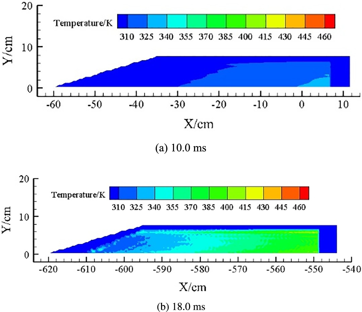
Figure 10: Temperature clouds with a bottom gap thickness of 0.00 cm

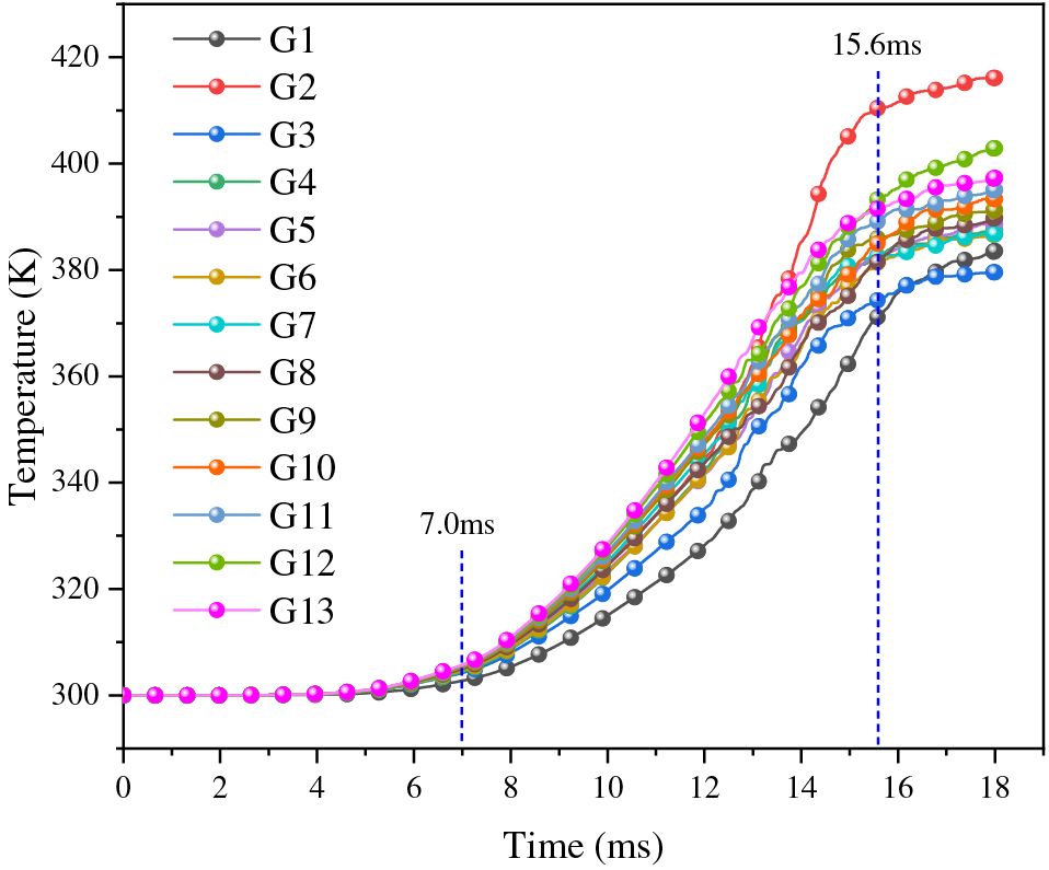
Figure 11: Temperature curve with a bottom gap thickness of 0.00 cm

Fig. 11 shows that the explosive bottom temperature increases slowly until 7.0 ms. In the early stages, the pressure load at the artillery bottom is relatively small, as is the pressure on the explosive bottom. Friction subsequently generates little heat, resulting in a slow increase in the explosive temperature. From 7–15.6 ms, the explosive temperature rises rapidly. As the pressure load at the artillery bottom increases, the pressure in the explosive bottom quickly rises, and friction generates more heat, resulting in rapid growth in the explosive temperature. The maximum temperature of 328.5 K occurs at point G13 at 10.0 ms. After 15.6 ms, the explosive temperature rises slowly. Ultimately, the temperature of the explosive bottom reaches a maximum of 416.1 K at point G2 at 18.0 ms.

(2) Bottom gap thickness of 0.01 cm

Figs. 12 and 13 show the temperature change of the COM B explosive charge under pressure loading with a bottom gap thickness of 0.01 cm. From Fig. 12a, the temperature gradually decreases from the explosive bottom to the explosive top at 10.0 ms. The maximum temperature region is mainly concentrated around the explosive bottom, where the temperature ranges of from 325–340 K, and the maximum temperature occurs at the center of the bottom of the COM B explosive charge. The temperature increases with time under the pressure loading action. Fig. 12b shows maximum temperature region remains around the explosive bottom at 18.0 ms, where the temperature ranges from 400–445 K. However, the maximum temperature point has shifted to the upper-left part of the explosive bottom.

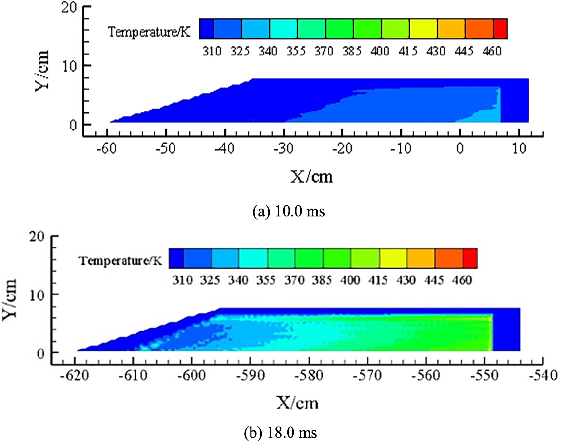
Figure 12: Temperature clouds with a bottom gap thickness of 0.01 cm

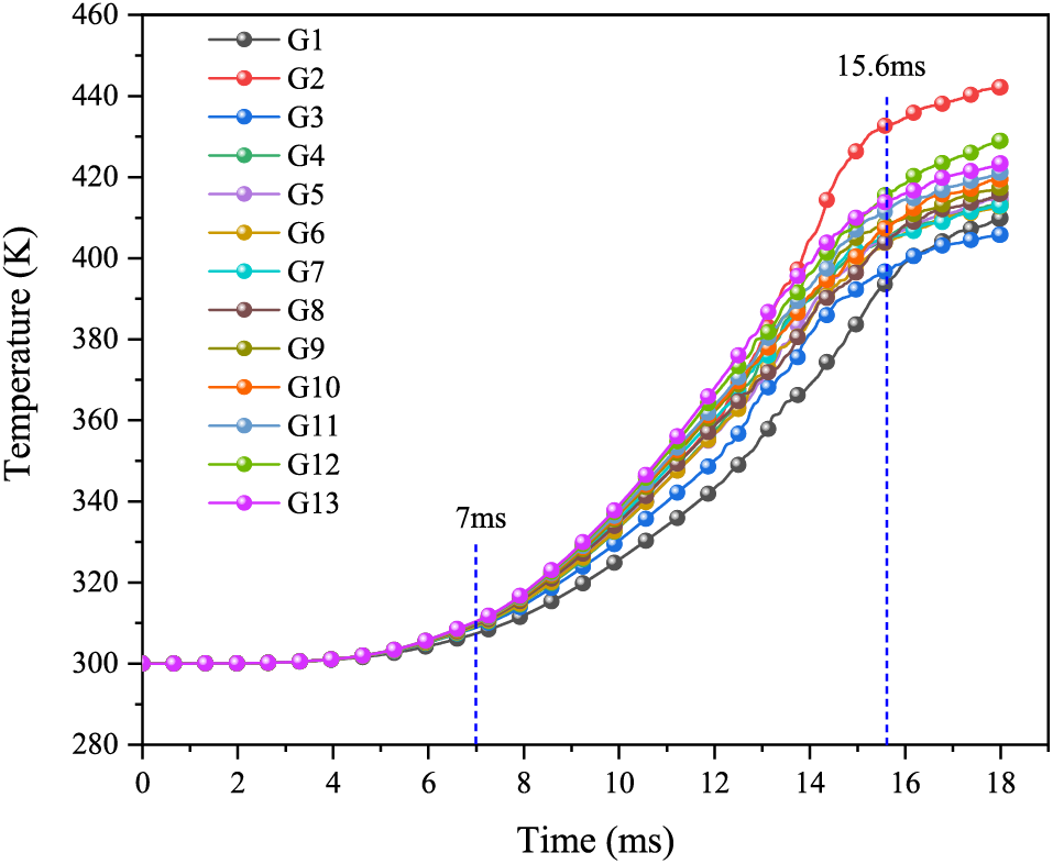
Figure 13: Temperature curve with a bottom gap thickness of 0.01 cm

As shown by Fig. 13, the explosive bottom temperature increases slowly until 7.0 ms. As the air in the bottom gap is compressed under the pressure loading, the air temperature rises, which causes the temperature of the explosive bottom to increase. A higher air temperature produces a higher temperature in the explosive bottom. In the early stages, the pressure loading at the artillery bottom is relatively small, and so the air is only slightly compressed. Less heat is generated by air compression and explosive crack friction, so the explosive temperature grows slowly. From 7–15.6 ms, the explosive temperature rises rapidly. As the pressure loading at the artillery bottom increases, the air is quickly compressed. Subsequently, the air compression and the explosive crack friction produce more heat, which leads to a rapid increase in the explosive temperature. At 10.0 ms, the maximum temperature of 339.1 K occurs at point G13. After 15.6 ms, the explosive temperature rises slowly. The reason for this phenomenon is the same as for the initial 7.0 ms. Ultimately, the temperature of the explosive bottom reaches a maximum of 442.2 K at point G2 after 18.0 ms. Compared with the case of no bottom gap, the maximum temperature at the same time is significantly higher with a bottom gap thickness of 0.01 cm. This indicates that the existence of the bottom gap is conducive to raising the temperature of the explosive bottom in the launch environment.

(3) Bottom gap thickness of 0.02 cm

Figs. 14 and 15 show the temperature change of the COM B explosive charge under pressure loading with a bottom gap thickness of 0.02 cm. From Fig. 14a, we find that the temperature gradually decreases from the explosive bottom to the explosive top at 10.0 ms. The maximum temperature region has a temperature range of 325–355 K and is mainly concentrated around the explosive bottom. The maximum temperature occurs at the center of the bottom of the COM B explosive charge. The temperature increases with time under the pressure loading action. From Fig. 14b, the maximum temperature region at 18.0 ms has a temperature range of 415–475 K and remains around the explosive bottom. However, the maximum temperature point has shifted to the upper-left part of the explosive bottom.

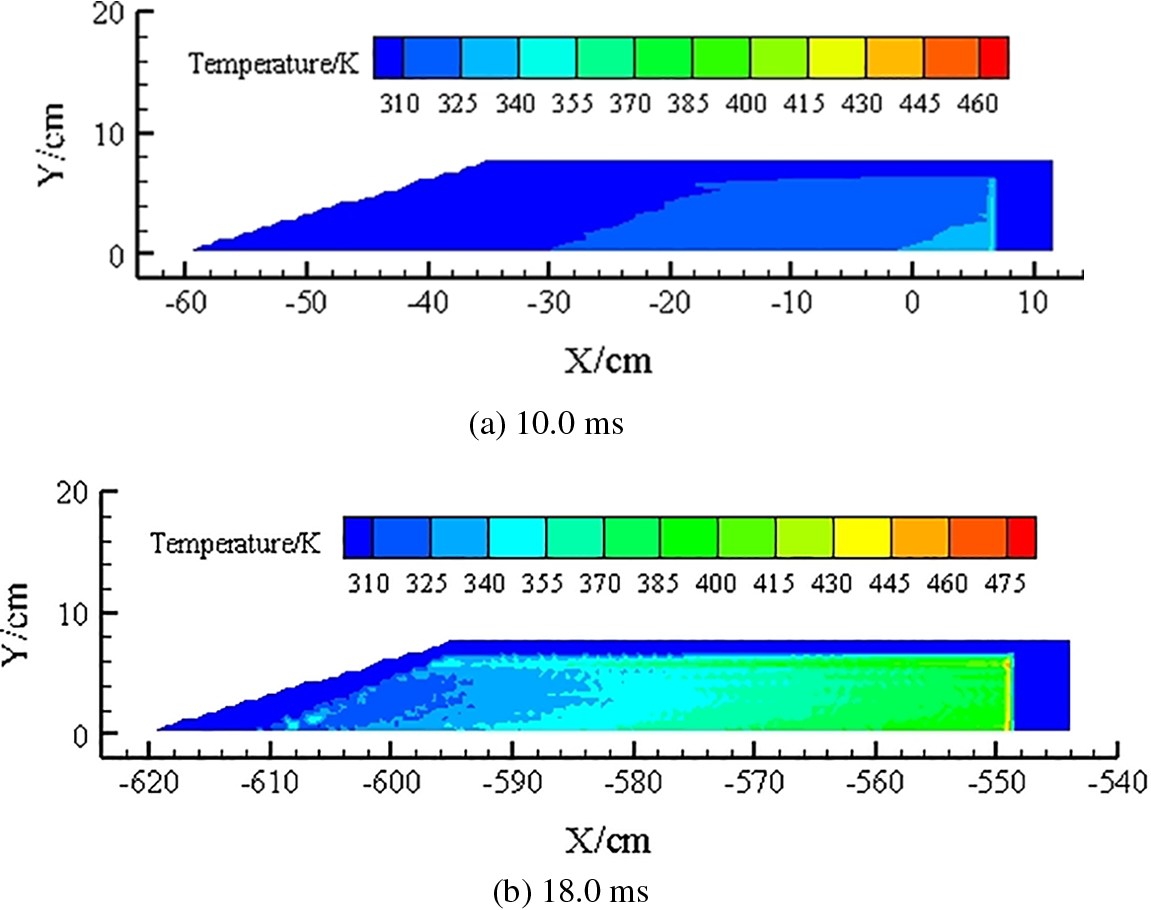
Figure 14: Temperature clouds with a bottom gap thickness of 0.02 cm

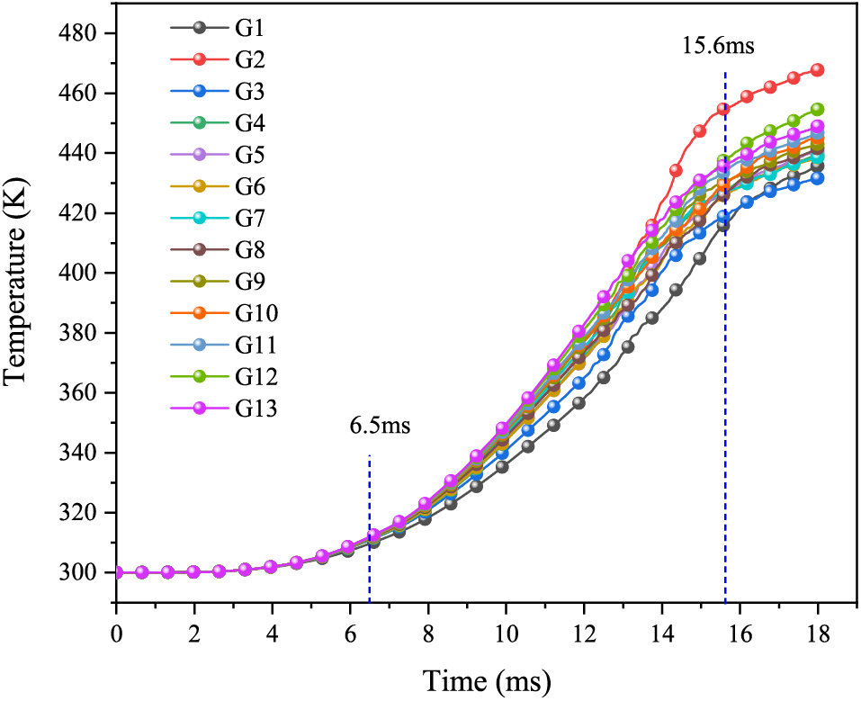
Figure 15: Temperature curve with a bottom gap thickness of 0.02 cm

From Fig. 15, the explosive temperature grows slowly until 6.5 ms. Afterward, the temperature increases rapidly. At 10.0 ms, the maximum temperature is 350.4 K at point G13. After 15.6 ms, the explosive temperature rises slowly. Ultimately, the temperature of the explosive bottom reaches a maximum of 467.7 K at point G2 after 18.0 ms.

(4) Bottom gap thickness of 0.03 cm

Figs. 16 and 17 show the temperature change of the COM B explosive charge under pressure loading with a bottom gap thickness of 0.03 cm. From Fig. 16a, the temperature gradually decreases from the explosive bottom to the explosive top at 10.0 ms. The region of maximum temperature (in which the temperature ranges from 340–370 K) is mainly concentrated around the explosive bottom, and the maximum temperature point is at the center of the bottom of the COM B explosive charge. The temperature increases with time under pressure loading. Fig. 16b shows that the maximum temperature region remains at the explosive bottom at 18.0 ms, and the temperature range in this area is 445–505 K. However, the maximum temperature point has shifted to the upper-left part of the explosive bottom.

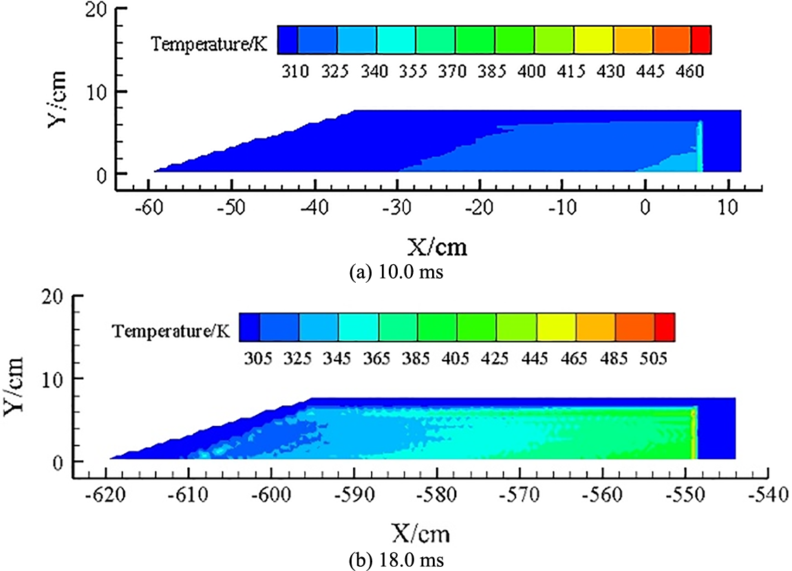
Figure 16: Temperature clouds with a bottom gap thickness of 0.03 cm

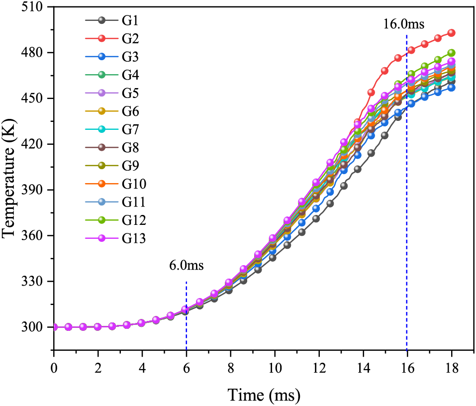
Figure 17: Temperature curve with a bottom gap thickness of 0.03 cm

From Fig. 17, the explosive temperature rises slowly until 6.0 ms. Subsequently, the temperature increases rapidly. At 10.0 ms, the maximum temperature is 360.1 K at point G13. After 16.0 ms, the explosive temperature rises slowly. Ultimately, the temperature of the explosive bottom reaches a maximum of 492.9 K at point G2 after 18.0 ms.

(5) Bottom gap thickness of 0.039 cm

Figs. 18 and 19 show the temperature change of the explosive charge under pressure loading with a bottom gap thickness of 0.039 cm. From Fig. 18a, the temperature gradually decreases from the explosive bottom to the explosive top at 10.0 ms. The region of maximum temperature, ranging from 340–370 K, is mainly concentrated around the explosive bottom, and the maximum temperature occurs at the center of the bottom of the COM B explosive charge. The temperature increases with time under the pressure loading action. Fig. 18b indicates that the maximum temperature region is still around the explosive bottom at 18.0 ms, where the temperature ranges from 445–525 K. However, the maximum temperature point has shifted to the upper-left part of the explosive bottom.

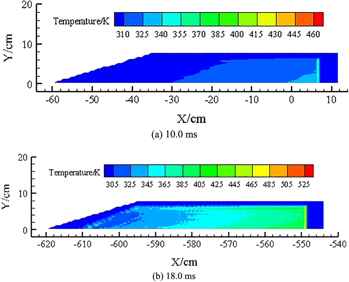
Figure 18: Temperature clouds with a bottom gap thickness of 0.039 cm

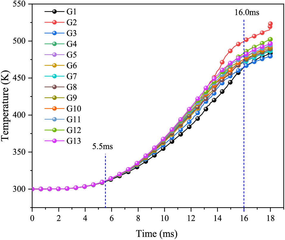
Figure 19: Temperature curve with a bottom gap thickness of 0.039 cm

From Fig. 19, the explosive temperature increases slowly until 5.5 ms, whereupon the temperature increases rapidly. At 10.0 ms, the maximum temperature is 369.5 K at point G13. After 16.0 ms, the explosive temperature rises slowly. Ultimately, the temperature of the explosive bottom reaches a maximum of 523.3 K at point G2 with a temperature after 18.0 ms.

(6) Bottom gap thickness of 0.04 cm

Figs. 20 and 21 show the temperature change of the explosive charge under pressure loading with a bottom gap thickness of 0.04 cm. From Fig. 20a, we see that the temperature gradually decreases from the explosive bottom to the explosive top at 10.0 ms. The maximum temperature region, where the temperature ranges from 340–370 K, is mainly concentrated around the explosive bottom, and the maximum temperature occurs at the center of the bottom of the COM B explosive charge. The temperature increases with time under the pressure loading action. In Fig. 20b, the maximum temperature region, in which the temperature ranges from 472–824 K, remains around the explosive bottom at 17.7 ms. However, the maximum temperature has shifted to the upper-left part of the explosive bottom. The complete combustion temperature is 784 K in the simulation process. This means that the combustion reaction occurs at the explosive bottom after 17.7 ms and the explosive charge is in an unsafe state during the launch process.

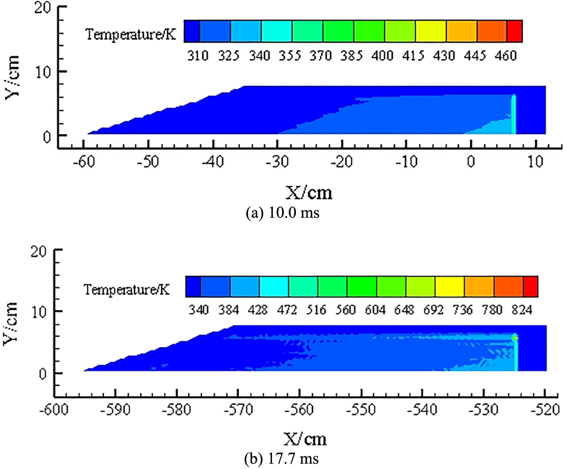
Figure 20: Temperature clouds with a bottom gap thickness of 0.04 cm

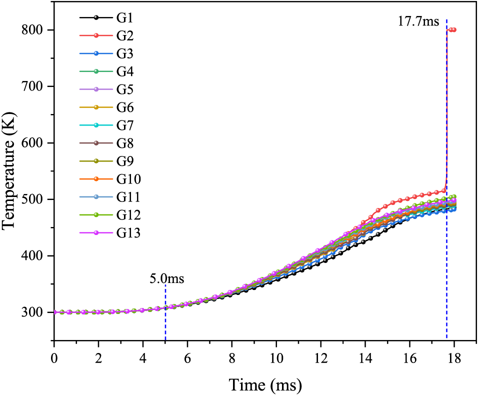
Figure 21: Temperature curve with a bottom gap thickness of 0.04 cm

Fig. 21 shows that the explosive temperature rises slowly until 5.0 ms and increases rapidly thereafter. The maximum temperature at 10.0 ms is 370.5 K at point G13. The explosive temperature suddenly increases to 800 K at 17.7 ms. The first point at which combustion occurs is G2 where the temperature is 800 K.

4.2.2 Discussion

Table 8 describes the influence of the bottom gap thickness on the maximum temperature of the COM B explosive charge in the launch environment. The maximum temperature region, which contains the maximum temperature point G2, is mainly concentrated around the explosive bottom. This indicates that the bottom gap thickness does not affect the location of the maximum temperature region or the maximum temperature point. The air contained in the bottom gap is compressed during the launch process of the artillery, causing its temperature to rise. The heat in the air is transferred to the explosive bottom, accelerating the rise in the temperature of the explosive bottom, while other parts of the explosive charge do not receive heat from the air. Therefore, the temperature of the explosive bottom is higher than the temperature of the other parts of the explosive charge. As the bottom gap thickness increases, more heat from the air is transferred to the explosive bottom, further enhancing its temperature. The bottom gap thickness only affects the temperature of the explosive bottom; it does not influence the location of the maximum temperature region or the point at which the maximum temperature occurs.

When the bottom gap thickness is 0.00 cm (i.e., no bottom gap), the explosive temperature increases with time under the pressure loading action and the maximum temperature reaches 416.1 K. In comparison, the maximum temperature is significantly higher when there is a nonzero the bottom gap. The bottom gap has a considerable effect on the explosive temperature in the launch environment. Furthermore, the temperature increases as the bottom gap becomes larger. When the bottom gap thickness is from 0.0–0.039 cm, the maximum temperature of the COM B explosive charge does not exceed 530 K. Consequently, the COM B explosive charge does not ignite and is safe in the launch environment. When the bottom gap thickness is 0.04 cm, the maximum temperature of the COM B explosive charge exceeds 784 K. This suggests that the COM B explosive charge will undergo the combustion reaction, making the launch environment unsafe. Accordingly, the bottom gap thickness should not be greater than 0.039 cm to ensure the safety of the COM B explosive charge in the simulated pressure of 496 MPa. Reference [2] stated that the bottom gap should be less than 0.05 cm to avoid the COM B explosive charge from exploding during the firing process, while reference [23] concluded from underwater experiments that the COM B explosive charge can explode under a pressure of 500 MPa when the gap is no less than 0.038 cm. Reference [24] found that the maximum bottom gap with the COM B explosive charge should not exceed 0.0381 cm under a simulated pressure of 506 MPa. Thus, the conclusion of this paper is consistent to the results of previous studies [2,23,24], which verifies the correctness of the proposed model. This model can be used to obtain the maximum bottom gap thickness during the launch process when different explosive charges are in a safe state. The bottom gap thickness is taken as the basis for judging the launch safety of explosive charges. When the bottom gap thickness is greater than the critical value, explosive charges are in an unsafe state. The maximum temperature with the various bottom gap thicknesses is shown in Fig. 22. As the bottom gap increases in thickness from 0.00–0.039 cm, the maximum temperature of the COM B explosive charge rises. Based on the simulation results presented in this paper, their relationship can be fitted as

T=2702.1H+416.1H∈[0.00,0.0039](45)

where T is the maximum temperature of the COM B explosive charge, and H is the bottom gap thickness. The constant term 416.1 is the maximum temperature of the COM B explosive charge in the case of a gap thickness of 0.00 cm. The coefficient 2702.1 is related to heat transfer and can be obtained from Eq. (42).

Figure 22: Maximum temperature with different bottom gap thicknesses

Fig. 23 shows the temperature difference at the bottom of the explosive charge at different times. The temperature difference is the difference between the maximum and minimum temperatures of the explosive bottom at the same time. When the bottom gap thickness is 0.00–0.03 cm, the temperature difference is about 13.4 K at 10.0 ms and 36.1 K at 18.0 ms. This indicates that the temperature difference is not affected by the bottom gap thickness at the same point in time, but increases over time.

Figure 23: Temperature difference at the bottom of the explosive charge at different times

5  Conclusions

Taking the COM B explosive charge as the research object, a combustion model of explosive charges in the launch environment was established with the MPM using the thermal equilibrium equation, Visco–SCRAM model, and virial equation. The model has the advantages of traditional grid model, but eliminates the numerical difficulties arising from grid distortion and nonlinear convection terms. Therefore, the proposed model is more suitable for solving the problem of explosive charge launch safety in the presence of a bottom gap. Based on the ideal gas adiabatic compression equation, a relationship between the pressure and temperature of the residual gas in the bottom gap was derived. Subsequently, the changes in the COM B explosive charge temperature with respect to the bottom gap (0.00–0.04 cm) in the launch environment was simulated under constrained conditions. The bottom gap thickness should not be greater than 0.039 cm to ensure the safety of the COM B explosive charge in the launch environment. This conclusion is consistent with those of multiple studies [2,23,24], and thus verifies the correctness of the model. By further analyzing the simulation results, the location of the maximum temperature region and the maximum temperature point were identified, providing the basis for positioning the temperature monitoring points during the launch process. The maximum temperature of the COM B explosive charge increases with increasing bottom gap thickness over the range 0.00–0.039 cm, and a mathematical expression describing this relationship was derived. The temperature difference at the same point in time was found to be affected by the bottom gap thickness over the range 0.00–0.03 cm, but was observed to increases over time. Ultimately, this paper establishes a quantitative evaluation method for the launch safety of explosive charges. This model is the first application of the MPM to launch dynamics. Thus this study extends the application field of the MPM and provides a means of studying the launch safety of different explosive charges.

Acknowledgement: The authors would like to extend our deep gratitude to Zhenqing Wang and Mingwu Sun for their insightful discussions and valuable suggestions on the study.

Funding Statement: This work was supported by the Natural Science Foundation of Heilongjiang Province, China (LH2019A008).

Author Contributions: The authors confirm contribution to the paper as follows: study conception and design: S. Wu, W. Chen, L. Liu; data collection: J. Ma, X. Song, H. Meng; analysis and interpretation of results: S. Wu, S. Lu. J. Ma, W. Chen; draft manuscript preparation: S. Wu, S. Lu, X. Song, H. Meng. All authors reviewed the results and approved the final version of the manuscript.

Availability of Data and Materials: The data that support the findings of this study are available from the corresponding author upon reasonable request.

Conflicts of Interest: The authors declare that they have no conflicts of interest to report regarding the present study.

References

1. Liu, W., Wang, G., Rui, X., Gu, J., Zhao, X. (2020). A hotspot model for PBX explosive charge ignition in a launch environment. Combustion Science and Technology, 2(2), 1–19. https://doi.org/10.1080/00102202.2020.1849166 [Google Scholar] [CrossRef]

2. Li, W. B., Wang, X. M., Zhao, G. Z., Du, Z. H. (2001). The research of the effect of base gap on the stress of explosives and the lunching safety. Journal of Ballistics, 13(3), 64–67+72. https://doi.org/10.3969/j.issn.1004-499X.2001.03.013 [Google Scholar] [CrossRef]

3. Austin, R. A., Barton, N. R., Howard, W. M., Fried, L. E. (2014). Modeling pore collapse and chemical reactions in shock-loaded HMX crystals. 18th Joint International Conference of the APS Topical Group on Shock Compress of Condensed Matter, Seattle, WA. [Google Scholar]

4. Wu, Y., Huang, F. (2013). Experimental investigations on a layer of HMX explosive crystals in response to drop-weight impact. Combustion Science and Technology, 185(2), 269–292. https://doi.org/10.1080/00102202.2012.716108 [Google Scholar] [CrossRef]

5. Holian, B. L., Germann, T. C., Maillet, J. B., White, C. T. (2002). Atomistic mechanism for hot spot initiation. Physical Review Letters, 89(28), 285501. https://doi.org/10.1103/PhysRevLett.89.285501 [Google Scholar] [PubMed] [CrossRef]

6. Walley, S. M., Field, J. E., Greenaway, M. W. (2006). Crystal sensitivities of energetic materials. Materials Science & Technology, 22(4), 402–413. https://doi.org/10.1179/174328406X91122 [Google Scholar] [CrossRef]

7. Shah, A., Brindley, J., Griffiths, J., Mcintosh, A., Pourkashanian, M. (2004). The ignition of low-exothermicity solids by local heating. Process Safety & Environmental Protection, 82(B2), 156–169. https://doi.org/10.1205/095758204322972799 [Google Scholar] [CrossRef]

8. Xiao, Y., Li, Y., Wang, Z., Zhao, H., Sun, Y. (2019). A constitutive model for the shock ignition of polymer bonded explosives. Combustion Science and Technology, 191(3), 590–604. https://doi.org/10.1080/00102202.2018.1505880 [Google Scholar] [CrossRef]

9. Jia, X., Cao, P., Han, Y., Zheng, H., Wu, Y. et al. (2022). Microstructure characterization of high explosives by wavelet transform. Mathematical Problems in Engineering, 2022, 1–16. https://doi.org/10.1155/2022/3833205 [Google Scholar] [CrossRef]

10. Guo, H., Wu, Y., Huang, F. (2017). A hot spots ignition probability model for low-velocity impacted explosive particles based on the particle size and distribution. Mathematical Problems in Engineering, 2017(2), 1–10. https://doi.org/10.1155/2017/7421842 [Google Scholar] [CrossRef]

11. Wu, Y., Huang, F. (2011). A microscor predicting hot-spot ignition of granular energetic crystals in response to drop-weight impacts. Mechanics of Materials, 43(12), 835–852. https://doi.org/10.1016/j.mechmat.2011.08.004 [Google Scholar] [CrossRef]

12. Li, W., Yan, H., Zhang, Q., Ji, Y. H. (2010). Compression process of pore inside explosive charge in a warhead under launching load. Defence Science Journal, 60(3), 244. https://doi.org/10.14429/dsj.60.349 [Google Scholar] [CrossRef]

13. Jetté, F., Yoshinaka, A., Higgins, A., Fan, Z. (2003). Effect of scale and confinement on gap tests for liquid explosives. Propellants Explosives Pyrotechnics, 28(5), 240–248. https://doi.org/10.1002/(ISSN)1521-4087 [Google Scholar] [CrossRef]

14. Zhang, Q., Bai, C. H., Dang, H. Y., Yan, H. (2004). Critical ignition temperature of fuel-air explosive. Defence Science Journal, 54(4), 469–474. https://doi.org/10.14429/dsj.54.2060 [Google Scholar] [CrossRef]

15. Xu, H., Shi, B., Zhang, Q. (2018). A multitarget visual attention based algorithm on crack detection of industrial explosives. Mathematical Problems in Engineering, 2018(10), 1–11. https://doi.org/10.1155/2018/8738316 [Google Scholar] [CrossRef]

16. Zhang, Q., Hu, S., Liang, H. (2013). Effect of pore in composition-B explosive on sensitivity under impact of drop weight. Defence Science Journal, 63(1), 108–113. https://doi.org/10.14429/dsj.63.2321 [Google Scholar] [CrossRef]

17. Zhou, P. Y., Xu, G. G., Wang, T. Z. (2000). Ignition models of explosive charge subjected to setback impact. Chinese Journal of Explosives and Propellants, 23(1), 1–5. https://doi.org/10.3969/j.issn.1007-7812.2000.01.001 [Google Scholar] [CrossRef]

18. Zhou, P. Y., Xu, G. G., Zhang, J. Y., Wang, T. Z. (1999). The experimental study of lunching safety of modified Comp-B explosive charge. Chinese Journal of Explosives and Propellants, 22(4), 34–35. https://doi.org/10.3969/j.issn.1007-7812.1999.04.010 [Google Scholar] [CrossRef]

19. Liu, W., Wang, G. P., Rui, X. T., Li, C., Wang, Y. (2022). A test method for launch safety of explosive charge accurately simulating launch overload. Journal of Energetic Materials, 11(3), 1–21. https://doi.org/10.1080/07370652.2022.2108165 [Google Scholar] [CrossRef]

20. Yu, Y., Yan, H., Chen, W., Ma, J. (2021). Finite volume method for the launch safety of energetic materials. Shock and Vibration, 2021(3), 9609557. https://doi.org/10.1155/2021/9609557 [Google Scholar] [CrossRef]

21. Qiang, H., Liu, Y., Wang, D., Wang, X., Geng, B. et al. (2021). Numerical simulation study of composite solid propellant small scale gap test. AIP Advances, 11(1), 015051. https://doi.org/10.1063/5.0039853 [Google Scholar] [CrossRef]

22. Cheng, L., Mu, H., Ren, X., Wen, Y., Zeng, X. et al. (2022). Study on the detonation reliability of explosive trains with a micro-sized air gap. AIP Advances, 12(10), 105309. https://doi.org/10.1063/5.0113801 [Google Scholar] [CrossRef]

23. Xiao, Z. Z., Tian, Q. Z. (1995). Studies on the base gap of composition B by aquarium test. Explosion and Shock Waves, 15(2), 141–146. [Google Scholar]

24. Meyers, T. F., Hershkowitz, J. (1981). The effect of base gaps on setback shock sensitivities of cast composition B and TNT as determined by the NSWC setback-shock simulator. 7th Symposium (International) on Detonation, Annapolis, Maryland, USA. [Google Scholar]

25. Meng, L., Liang, W., Hou, W. (2005). Design of a sensor for testing the gap at the bottom of an explosive charge. 2005 International Symposium on Test and Measurement, China. [Google Scholar]

26. Yang, Y., Zhang, Y., Han, Y. (2007). A study on ultrasonic detecting technology for the base gap on the inner cone. 6th WSEAS International Conference on Instrumentation, Measurement, Circuits and Systems, Hangzhou, China. [Google Scholar]

27. Cui, X. X., Zhang, X., Sze, K. Y., Zhou, X. (2013). An alternating finite difference material point method for numerical simulation of high explosive explosion problems. Computer Modeling in Engineering & Sciences, 92(5), 507–538. https://doi.org/10.1007/s13235-012-0057-4 [Google Scholar] [CrossRef]

28. Kakogiannis, D., Van Hemelrijck, D., Wastiels, J., Palanivelu, S., Van Paepegem, W. et al. (2010). Assessment of pressure waves generated by explosive loading. Computer Modeling in Engineering & Sciences, 65(1), 75–93. https://doi.org/10.2478/s11533-010-0040-5 [Google Scholar] [CrossRef]

29. Souli, M., Bouamoul, A., Nguyen-Dang, T. V. (2012). Ale formulation with explosive mass scaling for blast loading: Experimental and numerical investigation. Computer Modeling in Engineering & Sciences, 86(5), 469–486. https://doi.org/10.1061/(ASCE)MT.1943-5533.0000478 [Google Scholar] [PubMed] [CrossRef]

30. Liang, Y., Zhang, X., Liu, Y. (2019). An efficient staggered grid material point method. Computer Methods in Applied Mechanics and Engineering, 352, 85–109. https://doi.org/10.1016/j.cma.2019.04.024 [Google Scholar] [CrossRef]

31. Nairn, J. A., Guilkey, J. E. (2014). Axisymmetric form of the generalized interpolation material point method. International Journal for Numerical Methods in Engineering, 101(2), 127–147. https://doi.org/10.1002/nme.4792 [Google Scholar] [CrossRef]

32. Zhang, F., Shen, F., Li, B., Yuan, B., Li, B. et al. (2020). A comparison investigation on cylinder test in different ambient media by experiment and numerical simulation. International Journal of Aerospace Engineering, 2020, 1–12. https://doi.org/10.1155/2020/8874619 [Google Scholar] [CrossRef]

33. Narin, B., OEzyoeruek, Y., Ulas, A. (2014). Two dimensional numerical prediction of deflagration-to-detonation transition in porous energetic materials. Journal of Hazardous Materials, 273, 44–52. https://doi.org/10.1016/j.jhazmat.2014.03.027 [Google Scholar] [PubMed] [CrossRef]

34. Shie, Y. (2014). Dynamic fracture in thin shells using meshfree method. Mathematical Problems in Engineering, 2014(2), 1–8. https://doi.org/10.1155/2014/262494 [Google Scholar] [CrossRef]

35. Rabczuk, T., Belytschko, T. (2004). Cracking particles: A simplified meshfree method for arbitrary evolving cracks. International Journal for Numerical Methods in Engineering, 61(13), 2316–2343. https://doi.org/10.1002/nme.1151 [Google Scholar] [CrossRef]

36. Rabczuk, T., Belytschko, T. (2007). A three-dimensional large deformation meshfree method for arbitrary evolving cracks. Computer Methods in Applied Mechanics and Engineering, 196, 2777–2799. https://doi.org/10.1016/j.cma.2006.06.020 [Google Scholar] [CrossRef]

37. Ren, B., Li, S. (2012). Modeling and simulation of large-scale ductile fracture in plates and shells. International Journal of Solids and Structures, 49(18), 2373–2393. https://doi.org/10.1016/j.ijsolstr.2012.04.033 [Google Scholar] [CrossRef]

38. Fan, H., Li, S. (2017). A Peridynamics-SPH modeling and simulation of blast fragmentation of soil under buried explosive loads. Computer Methods in Applied Mechanics and Engineering, 318(2), 349–381. https://doi.org/10.1016/j.cma.2017.01.026 [Google Scholar] [CrossRef]

39. Fan, H., Li, S. (2017). Parallel peridynamics-SPH simulation of explosion induced soil fragmentation by using OpenMP. Computational Particle Mechanics, 4(2), 199–211. https://doi.org/10.1007/s40571-016-0116-5 [Google Scholar] [CrossRef]

40. Fan, H., Bergel, G. L., Li, S. (2015). A hybrid peridynamics-SPH simulation of soil fragmentation by blast loads of buried explosive. International Journal of Impact Engineering, 87(11), 14–27. https://doi.org/10.1016/j.ijimpeng.2015.08.006 [Google Scholar] [CrossRef]

41. Samaniego, E., Anitescu, C., Goswami, S., Nguyen-Thanh, V. M., Guo, H. et al. (2020). An energy approach to the solution of partial differential equations in computational mechanics via machine learning: Concepts, implementation and applications. Computer Methods in Applied Mechanics and Engineering, 362(2), 112790. https://doi.org/10.1016/j.cma.2019.112790 [Google Scholar] [CrossRef]

42. Rabczuk, T., Ren, H., Zhuang, X. (2019). A nonlocal operator method for partial differential equations with application to electromagnetic waveguide problem. Computers, Materials & Continua, 59(1), 31–55. https://doi.org/10.32604/cmc.2019.04567 [Google Scholar] [PubMed] [CrossRef]

43. Ren, H., Zhuang, X., Rabczuk, T. (2020). A nonlocal operator method for solving partial differential equations. Computer Methods in Applied Mechanics and Engineering, 358(5), 112621. https://doi.org/10.1016/j.cma.2019.112621 [Google Scholar] [CrossRef]

44. Ren, H., Zhuang, X., Rabczuk, T. (2017). Dual-horizon peridynamics: A stable solution to varying horizons. Computer Methods in Applied Mechanics and Engineering, 318(4), 762–782. https://doi.org/10.1016/j.cma.2016.12.031 [Google Scholar] [CrossRef]

45. Gu, Y., Fu, Z. J., Golub, M. V. (2022). A localized Fourier collocation method for 2D and 3D elliptic partial differential equations: Theory and MATLAB code. International Journal of Mechanical System Dynamics, 2(4), 339–351. https://doi.org/10.1002/msd2.12061 [Google Scholar] [CrossRef]

46. Carpenter, H. J., Ghayesh, M. H., Zander, A. C., Psaltis, P. J. (2023). Effect of coronary artery dynamics on the wall shear stress vector field topological skeleton in fluid-structure interaction analyses. International Journal of Mechanical System Dynamics, 3(1), 48–57. https://doi.org/10.1002/msd2.12068 [Google Scholar] [CrossRef]

47. Jiang, K., Lu, X., Wang, H. (2022). Influence of multiple structural parameters on buffer performance of a thin-walled circular tube based on the coupling modeling technique. International Journal of Mechanical System Dynamics, 2(4), 374–390. https://doi.org/10.1002/msd2.12060 [Google Scholar] [CrossRef]

48. Andersen, S., Andersen, L. (2010). Analysis of spatial interpolation in the material-point method. Computers & Structures, 88(7–8), 506–518. https://doi.org/10.1016/j.compstruc.2010.01.004 [Google Scholar] [CrossRef]

49. Mason, M., Chen, K., Hu, P. G. (2014). Material point method of modelling and simulation of reacting flow of oxygen. International Journal of Computational Fluid Dynamics, 28(6–10), 420–427. https://doi.org/10.1080/10618562.2014.973406 [Google Scholar] [CrossRef]

50. Ma, J., Wang, D., Randolph, M. F. (2014). A new contact algorithm in the material point method for geotechnical simulations. International Journal for Numerical and Analytical Methods in Geomechanics, 38(11), 1197–1210. https://doi.org/10.1002/nag.2266 [Google Scholar] [CrossRef]

51. Bahri, A., Guermazi, N., Elleuch, K., Ürgen, M. (2016). On the erosive wear of 304 L stainless steel caused by olive seed particles impact: Modeling and experiments. Tribology International, 102(7), 608–619. https://doi.org/10.1016/j.triboint.2016.06.020 [Google Scholar] [CrossRef]

52. Wang, X., Shi, J. (2013). Validation of Johnson-Cook plasticity and damage model using impact experiment. International Journal of Impact Engineering, 60(10), 67–75. https://doi.org/10.1016/j.ijimpeng.2013.04.010 [Google Scholar] [CrossRef]

53. Johnson, G. R., Cook, W. H. (1985). Fracture characteristics of three metals subjected to various strains, strain rates, temperatures and pressures. Engineering Fracture Mechanics, 21(1), 31–48. https://doi.org/10.1016/0013-7944(85)90052-9 [Google Scholar] [CrossRef]

54. Chen, W., Wu, S., Ma, J., Liu, L., Lu, S. (2022). Numerical simulation of the deflagration to detonation transition behavior in explosives based on the material point method. Combustion and Flame, 238, 111920. https://doi.org/10.1016/j.combustflame.2021.111920 [Google Scholar] [CrossRef]

55. Chen, W., Ma, J., Shi, Y., Xu, C., Lu, S. (2018). A mesoscopic numerical analysis for combustion reaction of multi-component PBX explosives. Acta Mechanica, 229(5), 2267–2286. https://doi.org/10.1007/s00707-017-2098-7 [Google Scholar] [CrossRef]

56. Bennett, J. G., Haberman, K. S., Johnson, J. N., Asay, B. W. (1998). A constitutive model for the non-shock ignition and mechanical response of high explosives. Journal of the Mechanics and Physics of Solids, 46(12), 2303–2322. https://doi.org/10.1016/S0022-5096(98)00011-8 [Google Scholar] [CrossRef]

57. Liu, R., Chen, P. (2018). Modeling ignition prediction of HMX-based polymer bonded explosives under low velocity impact. Mechanics of Materials, 124, 106–117. https://doi.org/10.1016/j.mechmat.2018.05.009 [Google Scholar] [CrossRef]

58. Xiao, Y., Fan, C., Wang, Z., Sun, Y. (2020). Coupled mechanical−thermal model for numerical simulations of polymer−bonded explosives under low−velocity impacts. Propellants, Explosives, Pyrotechnics, 45(5), 823–832. https://doi.org/10.1002/prep.201900345 [Google Scholar] [CrossRef]

59. Liu, R., Chen, P., Zhang, X. (2020). Effect of continuous damage accumulation on ignition of HMX-based polymer bonded explosives under low-velocity impact. Propellants Explosives Pyrotechnics, 45(12), 1908–1919. https://doi.org/10.1002/prep.202000107 [Google Scholar] [CrossRef]

60. Yang, K., Wu, Y., Huang, F. (2018). Numerical simulations of microcrack-related damage and ignition behavior of mild-impacted polymer bonded explosives. Journal of Hazardous Materials, 356(12), 34–52. https://doi.org/10.1016/j.jhazmat.2018.05.029 [Google Scholar] [PubMed] [CrossRef]

61. Addessio, F. L., Johnson, J. N. (1990). A constitutive model for the dynamic response of brittle materials. Journal of Applied Physics, 67(7), 3275–3286. https://doi.org/10.1063/1.346090 [Google Scholar] [CrossRef]

62. Dienes, J. K., Kershner, J. D. (2000). Crack dynamics and explosive burn via generalized coordinates. Journal of Computer-Aided Materials Design, 7(3), 217–237. https://doi.org/10.1023/A:1011874909560 [Google Scholar] [CrossRef]

63. Murphy, M. J., Lee, E. L., Weston, A. M., Williams, A. E. (1993). Modeling shock initiation in Composition B. 10th Symposium on Detonation, Boston. [Google Scholar]

64. Dienes, J. K., Zuo, Q. H., Kershner, J. D. (2006). Impact initiation of explosives and propellants via statistical crack mechanics. Journal of the Mechanics and Physics of Solids, 54(6), 1237–1275. https://doi.org/10.1016/j.jmps.2005.12.001 [Google Scholar] [CrossRef]

65. McClelland, M., Glascoe, E., Nichols, A., Schofield, S., Springer, H. (2014). ALE3D simulation of incompressible flow, heat transfer, and chemical decomposition of Comp B in slow cookoff experiments. 15th International Detonation Symposium, San Francisco, CA, USA. [Google Scholar]

66. Hobbs, M. L., Kaneshige, M. J., Anderson, M. U. (2012). Cookoff of a melt-castable explosive (Comp-B). 27th Propulsion Systems Hazards Joint Subcommittee Meeting, Monterrey, CA, USA. [Google Scholar]

67. Liu, B., Vu-Bac, N., Zhuang, X., Fu, X., Rabczuk, T. (2022). Stochastic integrated machine learning based multiscale approach for the prediction of the thermal conductivity in carbon nanotube reinforced polymeric composites. Composites Science and Technology, 224, 109425. https://doi.org/10.1016/j.compscitech.2022.109425 [Google Scholar] [CrossRef]

68. Liu, B., Vu-Bac, N., Zhuang, X., Rabczuk, T. (2020). Stochastic multiscale modeling of heat conductivity of Polymeric clay nanocomposites. Mechanics of Materials, 142(268), 103280. https://doi.org/10.1016/j.mechmat.2019.103280 [Google Scholar] [CrossRef]

69. Dai, S. (2020). Physics of combustion and detonation of propellants and explosives. Beijing, China: National Defense Industry Press. [Google Scholar]

70. Zheng, J., Li, H. J., Wu, B. (2021). Fatigue failure and launch safety assessment of gun barrel. Proceedings of 2021 7th International Conference on Manufacturing Technology and Applied Materials, Sanya, China. [Google Scholar]

71. Zhang, Y., Zu, J., Zhang, H. Y. (2012). Environmental factors calibration technology of weapon chamber pressure test system. Fire Control & Command Control, 37(9), 209–213. https://doi.org/10.3969/j.issn.1002-0640.2012.09.056 [Google Scholar] [CrossRef]