Recent Advances of Deep Learning in Geological Hazard Forecasting

1  Introduction

Geological hazards are caused by endogenous and exogenous geological processes or anthropogenic factors on earth [1,2], which encompass a broad range of abnormal stratigraphic activity or extreme changes in geological environments, such as landslides, avalanches, debris flows, earthquakes, etc. Geological hazards pose a serious threat to human life and property [3]. Only by accurately forecasting the occurrence of geohazards can emergency measures be devised to mitigate the damage caused by the impending disaster. Geological hazard forecasting refers to the use of logical reasoning, numerical simulation, and comprehensive analysis based on historical geological hazard activity patterns, formation conditions, occurrence mechanisms, and other factors to speculate and assess the development and changes of geological hazards and the possible degree of danger and damage in a certain period in the future. Geohazard forecasting has attracted tremendous attention nowadays, particularly considering natural resource scarcity, environmental degradation, population expansion, sustainable development, and world economic integration.

Many efforts have been made in forecasting geological hazards in the past decades. The “3S technology”, including Global Position System (GPS), Geographic Information System (GIS) [4], and Remote Sensing (RS), has been widely applied in the field of geological hazard forecasting [5]. The Digital Disaster Reduction System (DDRS) [6], as a product of a high degree of integration between earth system science and information science, uses multidimensional virtual reality technology [7] based on mathematical and physical models to simulate the process of hazard occurrence and propagation. With the continuous progress of science and technology, various technical means such as synthetic aperture radar measurements [8], high-definition satellite remote sensing [9], aerial surveys by unmanned aerial vehicles [10], and airborne lidar measurements [11] are making new waves in the field of geological hazard forecasting.

The past decades have witnessed the revolutionary advancement of deep learning, which is a branch of machine learning that relies on artificial neural networks with three or more layers. In recent years, with the exponential growth of computational power and data sources, deep learning [12–14] has achieved tremendous success in a variety of applications. A growing number of studies have shown that deep learning techniques hold great promise for geohazard modeling and forecasting [15,16]. However, because deep learning originates from the areas of computer vision and natural language processing, when they are applied to the field of geohazard forecasting, the algorithm should be adapted or improved, for example by incorporating domain knowledge and conventional model-driven methods. The purpose of the paper is to provide systematic reviews of the advances and open issues associated with deep learning development in the field of geohazard forecasting.

As a status review paper, the article is intended to cover the following topics:

•   Current development and future trends of deep learning for geological hazards

•   Common technical means of acquiring geological hazard data

•   Model structures of frequently used neural networks

•   Causes and harms of common geological hazards

•   Typical applications of deep learning in geohazards

It is noted that many machine learning techniques that do not fall into the category of deep learning have been applied to geohazard forecasting and obtained good results in the problems such as regression, classification, and change detection [17], but the review in such techniques is beyond the scope of the present status review.

2  Fundamentals of Deep Learning Methods

2.1 Data Sources

As a data driven method, deep learning requires iterative categorization of features from large amounts of data, so data sources were once a hindrance to the development of deep learning. However, recent developments in technologies such as sensors [18] and remote sensing [19] have made large-scale data collection for geohazards easier.

•   Field trips. A large amount of available data can be obtained through fieldwork, especially the external features of geological hazards. For example, Guzzetti et al. [20] obtained the landslide inventory map through field mapping. With the rapid development of technology, this traditional approach is being gradually replaced due to its drawbacks of high time cost.

•   Drone. Drones have started to enter many traditional engineering fields in recent years [10,21]. They are typically equipped with multiple camera sensors, allowing for more detailed image analysis of the geologically hazardous area [22]. The most important feature of drone surveys compared to fieldwork is that they do not require significant labor costs. In addition to this, drones allow more information to be obtained in hazardous areas and have a high spatial resolution. Drones have now become a powerful tool in the field of geohazards for a rapid survey and detailed situation analysis of large areas affected by disasters. For example, Suh et al. [23] used drone measurements to map mine subsidence caused by hazardous mining at the Samsung Limestone Mine. Aerial photos and investigation of the post-disaster area were carried out in great detail.

•   Satellite data. Low Earth Orbit (LEO) satellite technology is well developed [24,25] and has provided a large amount of Earth observation data to the engineering field, leading to a significant increase in geohazard monitoring capabilities [26]. Four types of satellite data are commonly available [27]: Multispectral optical images for optical information analysis of the affected area [28]; High-resolution digital elevation model (DEM) [29]; Synthetic aperture radar images (SAR) [30] and interferometric synthetic aperture radar images (INSAR) [31]; GPS data for measuring surface deformation in the affected area [32].

•   Surveillance system. Currently, surveillance systems [33] are widely used in disaster-prone areas [34] to monitor surface movements [35], rainfall [36], etc. Compared to remote sensing techniques, surveillance systems can provide more information. Common monitoring devices include inclinometers [37] pore water pressure sensors [38], rain gauges [39], etc.

•   Artificial signal reflection. Seismic surveys generally model the subsurface space through the reflection and refraction of artificially emitted signals. The seismic reflection wave method [40] requires instrumentation consisting of three components: a seismic source, a receiving device, and a recording system. The single-channel continuous profile method and the multi-channel continuous profile method are the most commonly used methods for this technique, and sometimes the common-depth point reflection technique is used to improve the signal-to-noise ratio. Measurements of seismic reflection waves allow for a more accurate determination of the depth and morphology of the interface and the determination of local tectonics and stratigraphic lithology. In addition, groundwater [41] and resource exploration [42] studies can be applied to this approach.

2.2 Convolutional Neural Network

Convolutional Neural Networks (CNNs) [43,44] inspired by the principles of human vision, are a class of feed-forward neural networks that include convolutional computation and have a deep structure. It contains three main modules-a convolutional layer, a pooling layer, and a fully connected layer. A brief model of CNN is depicted in Fig. 1.

Figure 1: CNN

The convolutional layer is responsible for extracting local features from different locations of the original input or capturing intermediate features with learnable filters called kernels. These kernels can also be optimized for a given problem to reduce the gap between the actual layer and the output layer by optimization algorithms like backpropagation and gradient descent. The pooling layer can be considered as a subsampling layer that reduces the size of the input layer and specifies the maximum or average value of each subregion of the previous layer. Finally, after completing the alternating stack of convolutional and pooling layers, one or more fully connected layers are added for classification or feature representation purposes.

When multiple CNN are stacked together to capture local geometric or spatial patterns, it is referred to as a deep CNN [45]. Common mainstream CNNs architectures are AlexNet [46], VGGNet [47], ResNet [48], etc. CNN has the advantage of being able to learn advanced features by capturing ensemble and spatial features, but they are ineffective when dealing with overly complex data. Currently, CNNs are widely used for the segmentation of captured features and damage assessment of various geological hazards and are one of the most widely used deep learning models.

2.3 Recurrent Neural Network and LSTM

Convolutional neural networks can only process one input at a time and can only take into account the influence of the current input and not the influence of other momentary inputs. However, in geohazards, information from the previous moment or period is often required, which renders CNN powerless. This problem was solved by introducing recurrent neural networks.

Recurrent Neural Networks (RNNs) [49,50] are neural networks with hidden states, which change a two-dimensional neural network model, through hidden states, into a three-dimensional neural network model with time series. The structure of RNN is shown in Fig. 2. When dealing with large amounts of data, stacking many RNNs might cause gradient disappearance and explosion problems [51], long and short-term memory (LSTM) [52,53] was proposed to solve this challenge. LSTM implements information protection and control through three gate structures: the input gate, the forgetting gate, and the output gate. The principle of LSTM is shown in Fig. 3.

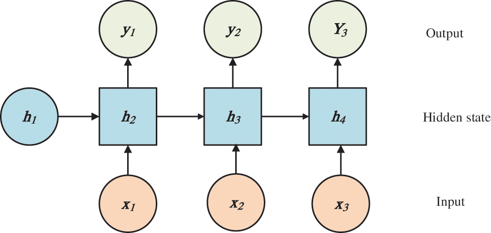
Figure 2: RNN

Figure 3: LSTM

Recurrent neural networks and LSTM are able to capture temporal dynamics, but often suffer from gradient disappearance [51] and short-term overdependence, and are unable to represent short-duration non-periodic data. They are currently commonly used in the temporal evolution of geological hazards, trend prediction and detection, and classification of infrastructure damage.

2.4 Autoencoder

Autoencoder (AE) [54] is an unsupervised learning model consisting of two main parts: Encoder and Decoder [55], as shown in Fig. 4. Depending on the learning paradigm, autoencoder can be classified as contractive autoencoder [56], regularized autoencoder [57] and variational Autoencoder [58]. The first two of them are discriminative models and the latter is a generative model. In terms of dimensionality reduction and denoising, AE provides certain advantages over traditional neural networks [59], and the features of the data can be extracted without tagging information. Furthermore, high-dimensional input data that cannot be handled by single-layer AE due to its simplistic structure can be solved by a stacked AE (SAE) architecture [60]. AE is now widely used for geohazard prediction and susceptibility analysis, and is often combined with LSTM to complete early warning systems.

Figure 4: AE

2.5 Generative Adversarial Network

Generative Adversarial Networks (GANs) [61] is a system consisting of two models: a discriminator and a generator, as shown in Fig. 5. The discriminator is typically built using a binary neural network to figure out whether the input image is from a dataset or created by a machine, usually treating samples extracted from the dataset as positives and generated samples as negatives. The generator’s task is to receive random noise and then use a deconvolutional network to create an image that can provide further training samples to the discriminator. The original GAN paper [62] used MLP to build the generative and discriminative models.

Figure 5: GAN

The aim of the GAN’s dual system is for the generator to attempt to confuse the discriminator while allowing the discriminator to make as many judgments as possible about the origin of the input image. The two models are in an adversarial relationship with each other and are iteratively optimized by gaming. After numerous rounds of training the discriminator and the generator, we hope that the distribution of the generator and the real samples will be identical and the discriminator will be unable to discriminate between them. In addition, providing other auxiliary information to the GAN can help improve its performance. Conditional generative adversarial networks (CGAN) [63] have been developed as a common variant of GAN, in which both generators and discriminators have the help of auxiliary information to reduce the randomness of the data. GAN, as a typical data generation model, is commonly used for data reconstruction of geohazards, especially for datasets containing large amounts of noise and missing values.

2.6 Graph Neural Network

Graph Neural Networks (GNNs) [64] are a class of deep learning-based methods for processing graph domain information. Due to its good performance and interpretability, GNN has recently become a widely used method for graph analysis. GNNs can obtain information such as neighboring regions of geohazards and spatial relationships between nodes and has unique advantages in cascading effects of geohazards. GNNs usually includes graph convolution networks [65], Graph Attention Networks [66], and Graph Autoencoders [67]. And the application of graph convolution networks is more common in the current geohazard research.

2.7 Deep Belief Network

As the following points show, traditional neural networks have many limitations that have stalled the development of neural networks for a while:

•   Primitive neural networks are generally single hidden layers [68], it has at most two hidden layers because once the number of neurons is too large and there are too many hidden layers, the number of parameters of the model grows rapidly and the model takes a very long time to train.

•   Traditional neural networks generally difficult to find the optimal solution with an increasing number of layers if stochastic gradient descent [69] is used, and they are easy to fall into local optimum solutions. It is also prone to gradient dispersion or gradient saturation in the backpropagation process, leading to unsatisfactory model results.

•   As the number of neural network layers increases, deep neural networks with many model parameters require a large amount of labeled data for training, because it is difficult to find the optimal solution when the training data is small, and although there are related studies [70], ordinary deep neural networks cannot solve small sample problems.

The emergence of deep belief networks has changed this trend. Deep Belief Networks (DBNs) [71] solve the optimization problem of deep neural networks by training layer by layer, assigning better initial weights to the entire network so that the network can be fine-tuned to reach an optimal solution. Playing the most important role in layer-by-layer training is the Restricted Boltzmann Machine (RBM) [72], as shown in Fig. 6. The Restricted Boltzmann Machine (RBM) is a simplification of the Boltzmann Machine (BM). A stack of multiple RBMs constitutes a DBN, where the output of the hidden layer of the previous RBM becomes the input to the visible layer of the next RBM [73] as shown in Fig. 7. The training of DBN is similar to that of an SAE in that the training process is performed layer by layer from low to high, where the initial parameters are learned in a layer-by-layer unsupervised mode so that additional layers are used at the top to fine-tune the parameters. There are no connections between the nodes in the same layer, which means that the visible units are independent [74]. This scheme allows learning a relatively better hierarchical representation, which can better reflect the underlying structure in the input data. Due to its better performance and parallel computing capabilities, DBN has recently become a widely used network in the field of geohazard prediction.

Figure 6: RBM

Figure 7: DBN

2.8 Physics-Informed Neural Network

CNN are a pure data-driven approach and lack physical prior knowledge, so in the engineering field where the mathematical models based on physical mechanism are well developed, the traditional numerical methods like the finite element method [75,76] and boundary element method [77,78] are still dominant. Physical Information Neural Networks (PINNs) [79] are a class of neural networks used to solve supervised learning tasks while incorporating physical laws described by partial differential equations (PDE). It is capable of learning not only the distribution laws of training data samples, as traditional neural networks do, but also the physical laws described by mathematical equations. This is achieved by adding the difference between the physical equations before and after the iteration to the loss function of the neural network so that the physical equations are also “involved” in the training process. Compared to purely data-driven neural network learning, PINN imposes physical information constraints on the training process and can therefore learn more general models with fewer data samples. Compared to traditional numerical analysis methods in engineering, PINN is still at a disadvantage in terms of accuracy and speed in approximating the solution of partial differential equations. On the other hand, PINN has the advantage of incorporating the data into the model and is much easier for conducting inverse analysis. Moreover, PINN can be viewed as a “meshfree” method, which alleviates the meshing burden in the finite element method.

2.9 Bayesian Neural Network

As mentioned previously in the introduction, unlike other fields where deep learning is common, the occurrence of geological disasters is full of uncertainties [80], restricting the practical applications of basic neural networks and common numerical methods. To quantify the impact of various uncertainty factors on the occurrence of geological hazards, deep learning needs to be employed in a unified probabilistic model. Bayesian network (BN) [81,82], also known as belief network or probabilistic directed acyclic graphical model, is a probabilistic graphical model that uses directed acyclic graphs (DAGs) to illustrate a set of uncertain variables and express their dependencies. The acyclic is designed to represent the flow of information in a way that can have a definite direction, if it is circular going this can produce some very troublesome things. The nodes of the network represent some random variables, an arrow between two nodes indicates that there is a relationship between the two nodes, some of which are observable and some of which are not. BNs have been applied to many engineering problems that operate under uncertainty. By using BNs, the joint probability distribution of a set of uncertain variables can be computed due to conditional independence and chaining rules. Through this thought, Bayesian Neural Networks (BNNs) incorporate some elements of probabilistic graphical models to compensate for the shortcomings of neural networks.

2.10 Meta-Heuristic Algorithm

Meta-heuristic algorithm (Meta-heuristic) [83–85] is a method for solving complex optimization problems based on the mechanism of computational intelligence to find optimal or satisfactory solutions, sometimes called intelligent optimization algorithm (Intelligent optimization algorithm) [86], intelligent optimization through the biological, physical, chemical, social, artistic and other systems or fields in the relevant behavior By understanding the relevant behaviors, functions, experiences, rules, and mechanisms of action in biological, physical, chemical, social, and artistic systems or fields, intelligent optimization reveals the design principles of optimization algorithms, refines the corresponding feature models under the guidance of specific problem characteristics, and designs intelligent iterative search-based optimization algorithms.

MH improves the traditional gradient optimization, but with relatively high computational complexity. Common optimization algorithms such as Genetic Algorithm (GA) is an evolutionary-based algorithm, Gray Wolf Optimizer (GWO) is a population behavior-based algorithm, etc. Ma et al. [87] conducted an extensive comparison among more than twenty MHs based on a case study of landslide displacement prediction, in which multiverse (MVO) has a good balance between accuracy, stability, and efficiency, and is highly competitive in the future, and in the paper, they also proposed a method based on k-fold cross-validation (K-fold CV), MHs and SVR (Support vector machines for regression analysis) hybrid method, which uses NMSE of K-fold CV set as an adaptation index for performance improvement, effectively improves the reliability and performance of geohazard modeling.

3  Application of Basic Neural Network in Geological Hazard

3.1 Seismic Analysis

Earthquakes [88–90] are geological hazards caused by the release of enormous energy from the Earth’s crust in a short period, its damage to the ground building is huge, as shown in Fig. 8. The collision of the Earth’s tectonic plates with each other [91] is the main cause of earthquakes, which cause dislocations and ruptures at the plate edges and within the plates. Over the past decade, researchers have been able to better study complex structures and dynamics deep within the Earth thanks to the large amount of data collected by numerous monitoring systems [92]. The following is a recent summary of seismic data interpolation and denoising as well as seismic detection and localization.

Figure 8: Earthquake

3.1.1 Seismic Data Interpolation and Denoising

Interpolation and denoising play a fundamental role in most seismic processing workflows. Seismic data interpolation [93] is a basic method to reconstruct lost recording channels, and denoising [94] separates or attenuates noise from the seismic signal. Inspired by the great contributions made in image processing and computer vision, CNNs can obtain a large amount of information by acquiring local features of images since most seismic data can be simply processed as images. For example, Wang et al. [95] combined seismic data interpolation with the image reconstruction problem by extracting high-level features of the training data through self-learning and successfully reconstructed periodically lost trajectories with high accuracy using an 8-layer ResNet-based model, demonstrating that CNN-based models can eliminate the linearity, sparsity, and low-order assumptions of traditional algorithms. Wu et al. [96] proposed a novel CNN-based self-supervised method to simultaneously attenuate seismic random noise and offset artifacts, called a self-adaptive denoising network (SaDN), which uses the assumption that synthetic noise with mixed Gaussian-Poisson distribution can simulate random noise and migration artifacts to modify the loss function of a denoising CNN (DnCNN) to adapt to different field data. Mandelli et al. [97] investigated a specific architecture based on convolutional neural networks, called U-Net [98,99], and implemented a convolutional self-encoder, which can reconstruct more complex seismic data more efficiently and accurately compared to traditional CNN models. To improve the performance of the U-Net. Tang et al. [100] added residual blocks to the deep U-Net, a model mainly used to process seismic data acquired through sparse 2D acquisition and named SRT2D-ResU-Net, and the reconstructed missing trajectories correlated with the true answers by more than 85\% on average. Huang et al. [101] trained a nested U-Net structure with mixed loss functions (U-Net++) to automatically generate pseudo labels to simulate continuous missing scenes by randomly masking the observed data so that local and global structural information can be captured to ensure reconstruction quality. Recently, blind spot (BS) strategies in image processing have attracted much attention. BS strategies allow one to estimate the denoiser from the noisy data itself. Fang et al. [102] proposed an unsupervised blind spot network (BSnet) method, in which two random mask operators are introduced to handle Gaussian white noise and bandpass noise, respectively, and the experimental results demonstrate the great potential of this strategy in the seismic field.

Seismic data in the temporal dimension cannot be represented by CNNs, so some researchers have started to consider seismic data as time series. For example, Yoon et al. [103] used five RNN-based deep learning models (basic RNN, LSTM, bi-directional LSTM, deep BiLSTM, and DBiLSTM with jump connections) for the reconstruction of seismic data, and the results demonstrated the usability of RNN and its derived models for reconstructing seismic data, but the drawback was that the correlation between multiple seismic traces could not be obtained.

In addition, GAN, a typical data generation model, can generate new seismic data from existing data distributions, and the generated seismic data can have the same distribution and features as the original data. For example, Kaur et al. [104] used the Cycle-GAN model, a derivative of GAN, to implement the reconstruction of missing trajectories from seismic data by creating training labels by randomly removing trajectories from different receiver indexes of the original dataset to simulate the effects of missing trajectories. Alwan et al. [105] developed a generator network (GANAN) based on U-Net [97], and the results demonstrated that GANAN can achieve more desirable results by processing noisy images into clear images. Furthermore, Wei et al. [106] used Wasserstein distance to train CGAN networks to improve the interpolation accuracy. Wasserstein distance can avoid gradient disappearance and pattern collapse so that the network successfully avoids low-rank, sparse or linear assumptions of seismic data. Dou et al. [107] proposed a multidimensional adversarial network that uses three discriminators to ensure that the distribution of the reconstructed data in each dimension is consistent with the original data, and embeds a feature stitching module (FSM) into the generator of this framework to provide maximum preservation of the original information.

Spectral analysis of seismic data is also an important research direction. To improve the interpolation accuracy, it is necessary to extend seismic data to the frequency domain. Chang et al. [108] proposed a new GAN (DD-CGAN) for interpolating seismic data in both time and frequency domains. DD-CGAN uses seismic datasets in the frequency domain and discrete Fourier transform datasets as input vectors, and the reconstructed seismic bands have a high degree of consistency with the actual trajectories. Feng et al. [109] developed a singular spectrum analysis-based novel denoising neural network, the Multichannel Singular Value Decomposition Denoising Convolutional Neural Network (SVDDCNN), which can simultaneously extract data features from the singular spectrum rather than the time domain and can obtain more accurate geophysical features, and helps to separate signals from noise.

Supervised learning-based approaches largely require a large training sample of high-quality labeled data, which hinders the generalization ability of the model. Fang et al. [110] considered that seismic data have good nonlocal self-similarity and used self-similarity blocks to rearrange the data and construct multiple pseudo-observations to achieve unsupervised training, allowing the study to get rid of the reliance on noiseless field data. Wang et al. [111] proposed an unsupervised denoising method that reduces the reliance on high-quality labeled data. The method is based on an improved network iterative soft thresholding algorithm (ISTA) that omits soft thresholds to mitigate the uncertainty introduced by the empirical choice of thresholds and enhances the generalization ability of the model.

3.1.2 Earthquake Detection and Location

CNNs are the most commonly used neural networks in earthquake detection and localization. Perol et al. [112] developed a CNN-based model called ConvNetQuake for earthquake detection, which is a highly scalable convolutional neural network for earthquake detection and localization from a single waveform. This model provides significant improvements in detection and localization accuracy compared to conventional seismic monitoring methods but is unable to classify seismic wave rows generated from the same source when a large number of seismic waves are received. To address this problem, McBrearty et al. [113] input seismic waveforms between two locations into a four-layer classical CNN and predict whether the waveforms are from the same or different sources for binary classification. In addition, Kriegerowski et al. [114] used a three-layer CNN to analyze full-waveform multichannel seismic records and completed the localization of the exact coordinate system.

CNNs have long been trained in a supervised manner using historical or synthetically generated datasets for earthquake source localization, but in recent years, PINN has been proposed as a new mainstream approach that effectively reduces the reliance on large amounts of labeled data. Yildirim et al. [115] proposed an approach for earthquake source localization based on the emerging PINN paradigm. Using the observed event P-wave arrival times and training the neural network by minimizing the loss function given by the mismatch between the observed and predicted travel times and the residuals of the eikonal equation, the source location is finally obtained by finding the location of the minimum travel time in the computational domain. Through comprehensive tests, the results demonstrate the effectiveness of the proposed method in obtaining robust earthquake source locations even in the presence of sparse travel time observations. This is due to the use of the eikonal residual term in the loss function, which acts as a physical information regularizer. Smith et al. [116] proposed a scheme for probabilistic seismic source inversion using Stein variational inference, a method that uses a differentiable forward model in the form of physics-informed neural networks, which are trained to solve the eikonal equation. The results prove to be very helpful in nucleating Stein variational iterative optimization particle ensembles to rapidly approximate the posterior without the need to build a walk-time table and to deal well with highly multi-peaked posterior distributions, which are common in seismic source inversion problems and have a very high potential for application. In addition, due to the advantages of graph neural networks, there are unique advantages to the earthquake source mechanism, for example, McBrearty et al. [117] trained graph neural networks to predict estimates directly from the input selected data. And each input allows for a variable number of stations and locations for different seismic networks, where the inputs include theoretical predictions of the data, given model parameters, and local elements of the adjacency matrix link space of the defined graph. The architecture uses one graph to represent the station set and another graph to represent the model space, and the model is experimentally shown to have unique advantages in inference, data fusion, and outlier suppression.

On the other hand, RNN and LSTM as typical time series models can capture the time-domain features of seismic signals. For example, Linville et al. [118] obtained features from spectrograms by CNN and LSTM, respectively. The results show that for the acquisition of event-related signals, the LSTM model performs better and can obtain correlations promptly. In addition, since RNN and its derived models can acquire temporal features, they can have more promising applications in the real-time detection of earthquakes in the future.

According to the relevant studies in recent years, hybrid models are one of the research trends in recent years. According to this idea, a hybrid model of CNN and RNN should be able to obtain more information from seismic data. Zhou et al. [119] treated seismic signals as a combination of non-sequential and sequential signals and detected seismic events from a 30-second-long three-component seismogram by an 8-layer CNN, and a two-layer bidirectional RNN to select P- and S-wave arrival times. Similarly, Bai et al. [120] trained an attention-based long short-term memory full convolutional network (LSTM-FCN) model that uses FCN to extract high-level features and LSTM to model temporal dependencies, improving the detection and localization accuracy of seismic events compared to the model alone. The advantages of both models are reflected in the hybrid model, but in this hybrid approach, the two models are trained in two separate steps.

End-to-end hybrid models are a good way to deal with the above difficulties. Instead of training each component in turn, all components in such models can be learned simultaneously [121], and this approach maximizes the amount of data that can be extracted while also improving performance [122]. Mousavi et al. [123] developed the CNN-RNN seismic detector (CRED), CRED cleverly blends the two models into a residual structure that allows the model to capture deeper and higher-level information while reducing computational complexity, and the results demonstrate that the model holds great promise for minimizing false alarm detection rates while reducing detection thresholds. Zhu et al. [124] proposed a new end-to-end architecture consisting of three sub-networks: the main network for extracting features from the original waveform, a phase pickup network based on P- and S-wave arrival selection based on extracted features, and an event detection sub-network that can be used for multi-station processing of seismic waveforms recorded on seismic networks. Another major advantage of hybrid models is that they can perform numerous related activities. simultaneously, making them more widely used in practice. Mousavi et al. [125] developed an end-to-end hybrid model called EQTransformer, which consists of an encoder and three independent decoders integrated with a CNN and unidirectional and bidirectional LSTM. The model accomplished both seismic detection and phase pickup, and its performance in both tasks was not weaker than that of a single model.

In addition, many scholars are investigating unsupervised learning for seismic detection, which can be used for unlabeled seismic events. For example, Seydoux et al. [126] developed an unsupervised framework for detecting and clustering seismic signals in continuous seismic data that combines a deep scattering network with a Gaussian mixture model to successfully process multiple complex seismic signals. Wang et al. [127] used CGAN and additional (seismic/non-seismic) label information to overcome the limitation of random samples generated by Gaussian noise, and the synthesized high-quality waveforms (seismic and non- The synthesized high-quality waveforms (seismic and non-seismic) increase the available training data and therefore improve the accuracy of the seismic event detection task.

Blasting is widely used in geoengineering projects, but improper blasting-induced ground vibrations expressed as PPV can pose a threat to the environment and residents, and to reduce the dangerous effects of blasting, Abbaszadeh Shahri et al. [128] used a generalized feedforward neural network (GFFN) structure combined with a novel automatic intelligent parameter setting method, using GFFN combined with firefly and imperialist competing metaheuristic algorithms (FMA and ICA) to develop two new optimized hybrid models, which have significantly improved the prediction accuracy for PPV in real detection events.

3.1.3 Prediction of Seismic Liquefaction

Seismic liquefaction [129,130] is the process by which an originally stable, predominantly solid-like sandy soil layer is transformed into an unstable mixed liquid under seismic action, resulting in a reduction in the support of the sandy soil layer. Before the earthquake, the saturated sandy soil body below the water table carried the weight of the soil and buildings above. Most of this weight is carried by the sandy soil particle skeleton like a spring, which presents a stable state. When an earthquake occurs, the tremendous energy inside the earth’s crust causes vibrations in a rapid release process, creating misalignments and ruptures in the interior and surface layers of the earth’s crust. The sandy soil below the groundwater level is instantly subjected to the strong action of the huge seismic force, the pore water in the sandy soil layer cannot be discharged quickly, and the pore pressure suddenly rises, resulting in the originally stable sandy soil layer to show liquid-like characteristics. The main disaster manifestations are surface cracking, sandblasting, and water bubbling, which leads to landslide and foundation failure, and puts buildings at risk of sinking, tilting, cracking [131], etc.

Due to the high cost and difficulty of collecting high-quality in-situ soil samples and testing granular soils, to evaluate soil liquefaction potential, geotechnical engineers normally adopt in situ testing or semi-empirical equations (liquefaction boundary curves) such as standard penetration tests (SPT) and cone penetration tests (CPT) based on machine learning methods [132]. For example, Karthikeyan et al. [133] used a correlation vector machine (RVM) based on SPT to determine the liquefaction trend of soil and compared it with an artificial neural network (ANN). Xue et al. [134] proposed a hybrid model based on a combination of support vector machines (SVM) and particle swarm optimization (PSO), and tested the robustness of the model based on CPT field data. and tested the ability of SVM in assessing liquefaction trends based on CPT field data, and the accuracy of the developed PSO-SVM approach exceeded many methods such as grid search by predicting the results.

But limited to SPT and CPT based, the relevant parameters are not sufficient to improve the performance of these models, shear wave velocity is a more important parameter to reduce field conditions and laboratory environment. For example, Zhang et al. [135] proposed a multilayer fully connected network (ML-FCN)) based on the shear wave velocity Vs and trained DNN models based on the dataset collected by Hanna et al. [136]. The DNN models were trained by Vs and SPT data in the dataset and demonstrated that high prediction accuracy could be achieved even without the Vs prediction model, while the presence of V s allowed the training rate to be unaffected.

In addition, plasticity index (PI) has considerable influence on measuring the liquefaction behavior of fine-grained soils on the liquefaction sensitivity of highly plastic soils. Ghani [137,138] and others compared Culture Algorithm (CA), Firefly Algorithm (FA), Genetic Algorithm (GA), Gray Wolf Optimizer (GWO), Particle Swarm Optimization (PSO) and Gradient-based optimizer (GBO) combined with artificial neural network for soil liquefaction assessment and concluded that PI and GBO based ANN models are a promising new tool and can help geotechnical engineers to be able to estimate the occurrence of liquefaction in the early stages of engineering projects.

3.2 Volcanic Activity Detection

Volcanic eruption [139] is a geological phenomenon that refers to the movement of the Earth’s crust accompanied by the release of magma and other ejecta from the crater to the surface within a short period, as shown in Fig. 9. About a quarter of the global population lives in the zone affected by volcanic activity, and according to statistics, volcanic eruptions have claimed the lives of about 270,000 people over nearly 400 years. In addition to the danger of volcanic activity itself, it can cause a variety of secondary hazards that may even have serious impacts on global transportation and the environment, in addition to causing distress to people in the areas involved [140], to reduce the negative effects of volcanic eruptions, identifying and monitoring volcanic activity is an effective approach [141,142].

Figure 9: Volcanic eruption

3.2.1 Classification of Volcanic Activity

Monitoring systems are now deployed at volcanoes around the world to monitor volcanic seismic events. Benefiting from this background, researchers have access to an increasing number of signals in the form of continuous data streams [143,144], and the rapid classification of collected volcanic seismic signals is crucial in eruption crisis scenarios.

As mentioned earlier, CNNs have shown excellent performance in the recognition and extraction of advanced features from images. The same idea applies to volcanic activity. Lara et al. [145] fed spectrograms generated by periodogram theory with different types of windows into a CNN with a recognition (detection +  classification) time response of about one minute, and the system performance showed 99% accuracy in the detection phase and 97% accuracy in the classification phase. Curilem et al. [146] converted spectrograms into 20 × 20 pixel RGB images fed into a simple CNN with only two convolutional layers and successfully classified various volcanic seismic source signals with an accuracy of over 95%. In addition, Canario et al. [147] compared the performance of three traditional neural network models, MLP, CNN, and LSTM, for signal classification and designed a new CNN-based model named SeismicNet. SeismicNet can directly input the acquired raw signals without converting them to images and ignores the preprocessing step. It successfully accelerates the classification of four types of volcanic events.

Similar to the difficulties encountered in seismic deep learning, high-performance deep learning models require a large number of high-quality labeled datasets. Another common solution to such problems is to introduce migration learning, using models already trained in different domains as starting points for the target model. For example, Titos et al. [148] used LeNet [149] as a feature extractor based on the idea of migration learning to effectively implement the classification of seismic-volcanic signals in a representative dataset containing regional earthquakes, volcanic tectonic earthquakes, long-period events, volcanic tremors, explosions, and collapses.

3.2.2 Detection of Volcanic Deformation

Volcanic activity and magma transport often lead to a series of surface deformation called volcanic deformation. The development of remote sensing technology provides a good opportunity for the development of volcanic deformation detection and alleviates the situation where volcanic activity cannot be detected due to a lack of data. The large coverage of satellite image data provides more data for learning volcanic activity detection in remote areas where in situ monitoring is not possible [140]. InSAR data commonly used today contain multiple interferometric stripe maps, which are ideal inputs for deep learning studies and are suitable for edge detection in CNNs.

Based migration learning strategy. Anantrasirichai et al. [150] used a pre-trained AlexNet for the accurate classification of interference stripes. However, the CNN-based model is easily classified as volcanic deformation when atmospheric signals are shown as stripes in the plot, which can lead to false positives and cause problems for the recognition task. To address this issue, Brengman et al. [151] developed a CNN-based derivative model, SarNet, to detect, localize, and classify the presence of isoseismic surface displacements in interferograms, and used a class activation map (CAM) to show where SarNet returned surface deformations in the interferogram with an overall accuracy of 85.22% in the actual interferogram, and SarNet returns the location of the surface deformation in the interferogram.

To improve the ability of CNN-based models to cope with this challenge, Anantrasirichai et al. [152] extended the sample by adding various atmospheric data to the real interferogram. The results showed that the performance of the model trained using synthetic interferograms was improved compared to the model trained using real interferograms alone. Thus, the application of data extension in detecting volcanic deformation proved to be promising.

3.2.3 Predictions of Volcanic Eruption

Thermal image of volcano observation are commonly used by monitoring stations to analyze the evolution of eruptive activity. However, the obtained thermal images are usually obscured by clouds and only intermittent image sequences can be obtained. To address this problem, Diaz et al. [153] used the architecture of convolutional LSTM (ConvLSTM) + Time-LSTM + U-Net to explicitly model intermittent image sequences, and the results had the lowest RMSE compared to common methods in experiments to predict the changes of volcanic temperature data.

An alternative approach to thermal image is Muography [154]. Muography is an imaging technique that visualizes the internal structure of active volcanoes by using high-energy near-horizontal-access cosmic muons, making it possible to trace magmatic activity before eruptions. The first direct evidence of the experiment was obtained by studying the summit of Mount Asama, Japan [155], which shows that muography resolves volcanic structure more precisely than traditional geographic techniques. Nomura et al. [156] used muography data collected from 2014–2016 at Sakurajima volcano in Japan and CNN for data analysis and prediction due to the image data and compared it with models such as SVM to demonstrate the advantage of the CNN in terms of accuracy. In addition, continuous image data can be considered as time series data, and the combination of CNN and RNN or LSTM can improve the prediction performance. Rodrígue et al. [157] used time-frequency representations (TFR) from Bezymianny and Etna volcano data to obtain physical information, and through a Bayesian network strategy and a well-designed deep ConvLSTM architecture, they learn temporal dynamics from scattering coefficients or features. The effectiveness of migration learning switching between volcanoes is also verified in the article, setting a new specification for semi-supervised seismic volcano monitoring.

3.3 Landslide Prevention

Landslides are the most common geological hazard, they are responsible for at least 17% of natural disaster deaths worldwide [158,159], and have a significant economic and social impact [120], as shown in Fig. 10. Landslides are largely unavoidable and are typically caused by a combination of local geological conditions and triggering causes (e.g., weather or earthquakes) [3], which makes predicting when and where landslides will occur a difficult task. However, combining deep learning with publicly available Earth observation data holds promise for predicting the occurrence of landslides [35].

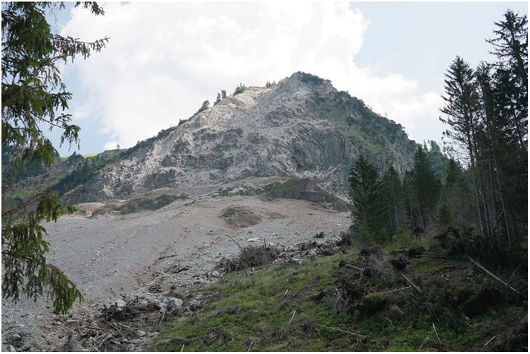
Figure 10: Landslide

3.3.1 Landslide Susceptibility Assessment

The goal of landslide susceptibility assessment aims to determine whether an area is susceptible to landslides based on available data [143], which typically include a wide range of local environmental factors and a history of previous hazards. Due to the powerful image feature extraction performance of CNNs, they can theoretically be directly applied to landslide susceptibility assessment. For example, Liu et al. [160] compared CNNs and traditional machine learning methods for landslide susceptibility mapping and demonstrated that both CNNs and traditional machine learning-based models have satisfactory performance, and CNNs achieved the highest performance. Youssef et al. [161] compared SVM, one-dimensional and two-dimensional CNNs and demonstrated that two-dimensional CNNs have the best performance compared to one-dimensional CNNs and SVMs. However, there are many differences between landslide susceptibility evaluation and image processing in practical engineering. Therefore, to effectively utilize the feature capture capability of CNNs, it is necessary to process landslide data into appropriate data types. Chen et al. [162] proposed a channel extension of pre-trained CNN and a traditional machine learning model (CPCNN-ML) based on The model that modifies a structurally mature pre-trained CNN to tap advanced features in the multichannel susceptibility layer, and the combination with random forest can improve reliability prediction. For example, Fang et al. [163] considered a stacked landslide map as a “multichannel image”, where each channel represents an environmental trigger, and then feed this “multichannel image” into CNN to obtain local features of the landslide, and then use the traditional machine learning methods as classifiers. The results show that the performance is improved compared to a single CNN model.

To more accurately assess landslide susceptibility, multi-scale spatial information on landslides needs to be considered. Yi et al. [164] proposed a multiscale sampling strategy that fuses multi-scale information around space to generate a dataset that is used as input to CNN. Compared with other neural networks, CNN has better fitting and prediction capabilities, and spatial data close to landslide locations are more suitable for predicting the probability of landslide occurrence. Hajimoradlou et al. [165] introduced U-Net for feature extraction in landslide susceptibility assessment, which has a more accurate susceptibility assessment compared to common CNNs. In addition, the proper setting of deep learning hyperparameters is also crucial for performance improvement. Sameen et al. [166] used Bayesian optimization to determine hyperparameters, and the prediction accuracy of CNN was improved by 3%. In addition, due to some background factors, some other things around, such as buildings, bare land, etc., bring challenges to the accuracy of detection. yang et al. [167] proposed Mask R-CNN with a background-enhancement method, and the model learns the difference between landslide and background objects more effectively by background-enhanced samples, thus reducing the false extraction of background objects.

Ngo et al. [168] used a basic CNN model and an RNN model to map landslide susceptibility, respectively, and the results proved that RNNs also have good performance. Therefore, RNNs were also introduced as time series models for landslide susceptibility assessment, and similar to CNNs, landslide data need to be processed into suitable time series data. For example, Mutlu et al. [169] formed a sequence by combining available landslide information with local location information and feeding it into RNN for further prediction. Wang et al. [170] made a comparison between conventional RNN and derived models, and several models have more ready prediction results with optimized parameters, proving the application prospect of RNNs.

Landslide susceptibility maps (LSM) have provided useful tools for decision-makers in recent years to mitigate disasters. Abbaszadeh Shahri et al. [171] developed a novel block-based hybrid neural network model (HBNN) to produce high-resolution LSM. This hybrid approach consists of an expert module structure and is combined with genetic algorithm (GA). By comparing multilayer perceptions (MLPs) and GFFN’s two developed models are compared and the relatively more reliable results demonstrate the ability of the developed HBNN to produce higher resolution and more reliable LSMs for urban and land use planners.

3.3.2 Landslide Displacement Prediction

Displacement prediction is a major application scenario of deep learning in landslide control. Displacement prediction focuses on the short-term behavior of landslides and provides an important basis for landslide warning systems. Typically, early warning systems mitigate potentially significant damage by providing actionable warning information about landslides before a disaster occurs [172].

Landslide deformation is a nonlinear dynamic process controlled by a complex environment, where the influencing factors and deformation behavior in the previous moment affect the deformation behavior in the next moment [173]. As predicting landslide deformation requires a logical relationship between moments, RNNs is the preferred model for displacement prediction. Typically, this model predicts dynamic landslide displacements by using data decomposed into static and dynamic components [173–177]. Jiang et al. [178] proposed a new graph convolution combined with a gated recurrent unit neural network (GRU) (GC-GRU-N), which applied the output of multi-weighted graph convolution to GRU to learn the time dependence, and the results showed that the model can effectively provide robust landslide displacement prediction. Zheng et al. [179] proposed an improved particle swarm IPSO-RNN landslide displacement prediction model based on RNN, which avoids artificial input hyperparameters, fits better, and has high prediction accuracy compared with the traditional landslide BP prediction model. Lin et al. [180] proposed the Double-BiLSTM model to calculate the correlation between the influencing factors and the periodic displacement using the maximum information coefficient (MIC) method, thus using the model for periodic displacement prediction. In addition, some other deep learning models can also achieve similar results. For example, Li et al. [181] used DBN to extract landslide displacement-related features from three denoised time series datasets without a priori knowledge and achieved satisfactory prediction performance. Theoretically, although DBN can extract correlation features from highly nonlinear and multivariate displacement data, it is difficult to capture temporal variations.

The performance of deep learning models in displacement prediction can be further enhanced by the proper application of diverse data. For example, Meng et al. [182] compared the performance of the model when using single- and multi-factor predictions and demonstrated that the latter reduced overfitting and improved accuracy. In addition, other effects besides rainfall and reservoir levels need to be considered, as well as interdependencies between different regions. Kuang et al. [183] proposed a novel GNN-based landslide prediction model that uses graph convolution to aggregate spatial correlations between different monitoring locations. The fusion of these features into a deep learning model can also be used to improve the accuracy of predicting landslide displacements.

3.4 Flood Prediction

As shown in Fig. 11, flooding [184,185] is one of the most frequent-occurring natural disasters, which is caused by heavy rainfall, rapid ice and snow melting, storm surge, etc. Moishin et al. [186] constructed a hybrid deep learning (ConvLSTM) algorithm based on various statistical score metrics, infographics, and visual analysis of forecast and real datasets. The evaluation results of the model are compared with the benchmark model, which demonstrates the applicability of this algorithm for short- and long-term flood scenario forecasting. Chen et al. [187] performed a similar study using ConvLSTM, but the importance of spatial features was emphasized in the paper by changing the input features to a two-dimensional time series spatial information, which experimentally proved to outperform most of the proposed models in terms of flood arrival times and peak flows. Hu et al. [188] integrated the LSTM and reduced-order model (ROM) framework to represent the spatiotemporal distribution of floods. To reduce the dimensionality of large spatial data sets in the LSTM, the paper introduces proper orthogonal decomposition (POD) to reduce the CPU cost by three orders of magnitude. By obtaining the time series of induced waves at the specified detectors, the use of LSTM-ROM can provide flood predictions within seconds, which has great practical significance. Sensitivity mapping is a key research area in flood prediction. Pham et al. [189] proposed a DBN deep learning algorithm based on an extreme learning machine (ELM) to obtain flood sensitivity mapping for the Vu Gia-Thu Bon watershed in central Vietnam. The proposed deep learning has the highest goodness-of-fit (AUC = 0.970) and prediction accuracy (AUC = 0.967) among all tested algorithm. Shahabi et al. [190] proposed a novel modeling approach (DBPGA) based on DBN) and Genetic Algorithm (GA) optimized Back Propagation (BP) algorithm for accurate flood sensitivity mapping for the Iranian Haraz Basin. Hosseiny et al. [191] used the U-Net model to analyze synthetic images, in which the input is from two bands of ground elevation and flood flow, and the output is the water depth. Based on the validation of field test data, the prediction of maximum flood depth for rivers was improved by 29%.

Figure 11: Flood

3.5 Debris Flow Detection

Debris flows are landslides that occur due to heavy rains, storms, or other natural disasters, transporting large amounts of boulders and silt [192], they frequently occur in canyon areas and areas prone to earthquakes and volcanoes, exploding rapidly without warning [193], as shown in Fig. 12.

Figure 12: Debris flow

Inspired by deep learning models in landslide sensitivity assessment, Zhang et al. [194] used an MLP and CNN-based model to convert external factors associated with mudflows into one-dimensional vectors as inputs to the model. The results showed that the model can effectively assess the probability of mudslides in a given region. Li et al. [195] combined CNN with two evolutionary optimization algorithms, Grey Wolf Optimizer (GWO) and Coyote Optimization Algorithm (COA) [196], and applied geoinformatics to the mudflow factor. The results showed that this approach has better fitting and prediction capabilities compared to CNN alone.

Ideally, information related to mudslides can be obtained using satellite image data. However, multispectral images are vulnerable to climate and high-resolution SAR images are too costly to be used on a large scale. To overcome these limitations, Yokoya et al. [197] cleverly solved this problem by combining numerical simulation methods with CNN-based Attention U-Net and LinkNet [198]. The numerical simulation method generates a large amount of data by simulating mudslide disaster scenarios, which satisfies the training requirements of CNN-based models and breaks the limitations of remote sensing.

The amount of sediment transported is an important but highly nonlinear dynamic process in water resources management, and Reza et al. developed two best prediction models subject to artificial neural networks (ANN) with different sensitivity analysis (SA) methods to prioritize the inputs used, resulting in a new, more efficient ANN structure, which, due to covering more uncertainty, uses SA’s parameter ranking would be more reliable. By processing 263 datasets from three rivers in Idaho, USA, it was found that the accuracy performance of the analysis using different criteria showed better predictability in the updated model, which could lead to a further understanding of the parameters used.

In addition, slope instability caused by water infiltration into soil is one of the important causes of debris flow and landslides, and the numerical study of water infiltration provides the conditions for the study. Yang et al. [199] combined partial differential equations of water infiltration and neural networks based on PINN to obtain a detailed numerical analysis of the water infiltration process, and the model error proposed in the paper is smaller compared with the traditional numerical methods, and the experimental results obtained in More accurate numerical results were obtained in the experiments.

3.6 Rockfall Prediction

Rockfall [200,201] occurs with high frequency in mountainous areas, generally due to slip or fracture phenomena of geotechnical bodies on steep slopes, as shown in Fig. 13. Because of the rapid occurrence of rockfalls, the difficulty of identifying them, and the complexity of the causal mechanisms, relevant studies are currently scarce. Since the Moon and Mars are similar to the Earth in terms of landslide principles, several current studies act on the prediction of rockfall on the Moon and Mars, which have some references for rockfall studies on Earth. For example, Bickel et al. [202] trained a CNN with residual blocks (RetinaNet) that can acquire salient features in images and generate a large number of rockfall maps, which are fundamental for the fast identification of rockfalls.

Figure 13: Rockfall

3.7 Avalanche Detection

When the internal cohesion of the snow on a mountain slope cannot resist the gravitational force, it slides downward, causing a massive snow collapse, i.e., so-call an avalanche, as shown in Fig. 14. They can occur in snow-covered areas all over the world. In the past decades, about 100 people have been killed in avalanches in the European Alps every year [203]. In addition, the damage to roads and infrastructure caused by avalanche is a major problem for people living in snow-covered mountain areas [204].

Figure 14: Avalanche

Traditional field methods are difficult to apply in practice, with time costs, high expenses, and hazards leading to the use of such methods only in small-scale disasters, and due to the large amount of data required for deep learning, which needs to be monitored continuously in time and space. The rapid development of satellite remote sensing has given a new opportunity for this research, and synthetic aperture radar is one of the more desirable sources of data acquisition. This is because avalanche detection requires the ability to capture pixel-level background information and multi-level features of avalanche debris, but traditional methods receive a large number of false positives due to climate and light effects, and synthetic aperture radar largely solves this problem by avoiding false detections of expected false positives.

Since the focus is on the background information around the pixel and extracting features, CNNs have now been applied to related research. Hafner et al. [205] proposed a fully convolutional neural network called AvaNet. AvaNet is based on the Deeplabv3+ (a commonly used semantic segmentation network) architecture and relies on manually mapped 24’737 avalanches for training, validation, and testing to achieve a more desirable level of prediction. Chen et al. [206] investigated stand-alone convolutional neural network models as well as two meta-heuristics including Grey Wolf Optimization (CNN-GWO) and imperialism applicability of the Competing Algorithm (CNN-ICA) in avalanches, analysis based on 13 potential drivers of avalanche occurrence and inventory plots of previously recorded avalanche occurrences, while the efficiency of model performance by the area under the receiver operating characteristic curve (AUC) And the root mean square error (RMSE) is evaluated, and the experimental results demonstrate the wide applicability of CNN in avalanche detection. Waldeland et al. [207] used a ResNet model trained on a natural image dataset to successfully identify candidate regions in The presence or absence of avalanche phenomenon. Also, since this work opportunities migration learning, itself an application in RGB images, this work converts the five channels of the input image into three channels through various combinations, with the red channel corresponding to the image of the avalanche event and the red and blue channels corresponding to the reference image. To improve the accuracy of CNN model detection, Sinha et al. [208] input SAR images and independent avalanche lists to a CNN-based CNN-based VGG-16 model, where the inventory contains the occurrence of avalanches, transformed from field data, and demonstrated the effectiveness of CNN-derived models for automatic avalanche debris detection by combining multiple information. Bianchi et al. [209] input two feature maps of SAR images and DEM The two feature maps of the DEM include slope angle features and angle of arrival. The SAR is fed into the model through an additional layer of the input image, while the DEM generates an attention mask from the attention module of the convolutional layer, allowing the model to focus more on the avalanche region.

Moreover, AE-based models have also shown good performance by identifying anomalies by comparing the compressed reconstructed data with the original data through the characteristics of AE. Again based on the idea of treating avalanches as rare events or anomalies and passing the variational autoencoder to isolate the anomalies, through this idea, Sinha et al. [210] demonstrated the usability of AE and its derivative models even beyond CNN models for avalanche detection by comparing AE-based models (VAE) with CNN models.

3.8 Drought Prediction

Drought [211] is a climatic phenomenon in which the total amount of fresh water is low and insufficient for human survival and economic development, generally over a long period, as shown in Fig. 15. Machine learning has proven to be useful in drought forecasting [212] and has been widely applied. Mishra et al. [213] and AghaKouchak et al. [214] in their article detail the various drought modeling methods used in the literature, and both emphasize that future research is directed toward developing more advanced models and assimilating data at higher time scales. Drought prediction has been greatly improved in some recent studies using lagged climate variables as predictors [215]. Despite the success of traditional machine learning, deep learning can improve the performance of drought prediction. Since droughts are long and slow, this means that they require models to process data in time series. In the current study, the RNN-derived model LSTM for recurrent neural networks to predict drought indices can handle real-time nonlinear data well and can help government departments to mitigate the influence of natural disasters. For example, Xu et al. [216] proposed a hybrid model based on a deep learning approach that integrates an autoregressive integrated moving average (ARIMA) model and long short-term memory (LSTM) model to improve the accuracy of short-term drought prediction. The prediction accuracy of ARIMA, support vector regression (SVR), LSTM, ARIMA-SVR, least squares SVR (LS-SVR), and ARIMA-6 drought prediction models were analyzed by comparing and contrasting, and the results showed that the model is more suitable for long-term drought prediction.

Figure 15: Drought

3.9 Others

There are many other geological hazards, such as ground subsidence [217], rock bursts [218], land desertification [219], geothermal damage [220], asteroid impacts [221], tornadoes [222], etc. Although most of these studies are still in their infancy, some fruitful research can already be seen. For example, Zhang et al. [223] proposed a ground subsidence prediction method, called the extended deep learning method. The method dynamically uses extended tunnel data to predict ground settlement in real time and proposes a kinetic correlation analysis method to evaluate the variable significance of input data on ground settlement based on static Pearson correlation coefficients by comparing four deep learning methods, including ANN, LSTM, GRU and one-dimensional convolutional neural network (Conv1d), and finally confirmed that the extended Conv1d model was able to accurately predict ground settlement due to tunnel boring with this approach, demonstrating the usability of this method. li et al. [224] applied Bayesian optimization and synthetic minority oversampling technique + Tomek Link (SMOTETomek) to efficiently develop a rockburst prediction feedforward neural network (FNN), where the model implements Bayesian optimization to find the best hyperparameters in the FNN and a balanced training set by employing SMOTETomek to eliminate the effect of unbalanced categories. To explain the FNN model, this work introduces the substitution importance algorithm to analyze the relative importance of the input variables, which has been shown to have good performance in real engineering experiments.

4  Challenges and Future Work

Despite enormous success of deep learning in geological hazards forecasting, many challenges remain to be resolved. In the following, we mention some possible directions worth of investigating in the future:

Uncertainty quantification. Uncertainty can be described as a situation involving incomplete or unknown information [225]. In general, three sources should be considered to quantify uncertainty [226], including the physical variability of the equipment, data and model errors. Traditional methods normally used statistical methods, polynomial chaos expansion method, Perturbation method and Monte Carlo simulation are common methods for uncertainty quantification. In deep learning, the Bayesian neural network is commonly used for uncertainty quantification. Feng et al. [227] used convolutional neural networks in a Bayesian framework to predict uncertainty in phase and quantification classification based on seismic data, using a variational approach to approximate the posterior distribution of mathematically intractable weights, and good experimental results demonstrated the effectiveness of the model. In addition, other methods in Bayesian theory-Markov Monte Carlo (MCMC), MC dropout (MCD), etc., also play an important role in assessing parameter uncertainty and model fitting. For example, Feng et al. [228] considered the importance of soil-water character curves (SWCC) for analyzing landslide seepage under different hydrodynamic conditions and developed a Bayesian updating framework developed from experimental data-used to investigate the uncertainty of SWCC parameters. In this proposed framework, the parameters of the model of SWCC are considered random variables, and MCMC is used to evaluate the parameter uncertainty, and the results prove that this framework is feasible for the observed data of large-scale landslide experiments. In the subsequent experiments, they build an ANN agent model, which greatly improves the efficiency of this Bayesian model update.

Bayesian theory is not the only approach used to quantify uncertainty; many other approaches have been proposed with good performance results. For example, Abbaszadeh Shahri et al. [226] proposed an Automatic Randomized De-Activation Connection Weight method (ARDCW), which is achieved by combining several derived sets from a fixed optimal topology. The framework uses nested loops to monitor all topologies with different hyperparameters to overcome the problem of overfitting and getting stuck in minima. After comparing with two UQ methods, MCD and quantile regression (QR), it has the most advanced performance.

Data sources. The basic problem in practical engineering challenges is the lack of data, and the inevitable missing and noisy data. Data quality issues are mitigated by data interpolation and denoising and deep learning model improvements, but the reliance on high-standard labeled data remains a challenge in the work. In addition, high equipment prices limit the areas where valid data are available, leaving many hazards to occur without relevant data available for study, creating a barrier to geohazard research in less developed regions. Open-source datasets have to some extent solved many of the team’s fundamental research problems [229–231], and although the number is relatively small at the moment, there are already several open-source projects driving this matter. Examples include the Climate Dataset (ERA5) [232] and the emergence of multi-hazard databases. Another approach is to perform data augmentation through models such as GAN or to train on small-scale data through migration learning [233]. In addition to the two approaches mentioned above, physical models and numerical simulations can be used to generate the required data, which can reduce the impact of missing data to a large extent.

In addition, in common studies today, good results are obtained on only one data source, but the actual data obtained is often a mixture of various data sources, which places higher demands on the performance of deep learning for classification and feature extraction, and hybrid models are a more powerful way to address such problems in the future. The future of geohazards is likely to be part of the geoscience data problem, requiring higher performance and more powerful models than are currently available.

Human activities. Except for earthquakes, most geohazards currently involve human activities [234,235], but the impact factors of human activities are complex and variable and require better models to measure them. There is also a lack of research on cascading effects between geohazards Studies of cascading effects between geological hazards is also lacking. Zuccaro et al. [236] described a theoretical model for cascading effects scenario analysis and a basic framework for identifying risk factors, including the interaction of geohazards leading to successive hazard events and the impact on the landscape and society.

The study of geological hazards is complex and requires more research breakthroughs based on the combination of basic deep learning methods because geological hazards are rapidly changing and their causes are complex, as mentioned in the previous article, how to label and classify the data obtained from geological hazards is a very important topic, and we believe that deep learning and more advanced data processing methods are important research directions in the future. However, the field of geohazards always needs human thinking to make key decisions, because methods including deep learning are based on past data to make the next inferences, but there are always more or fewer differences and new contents between geohazards and disasters.

We hope that more relevant practitioners will join the research in this area and grasp a major revolution brought by deep learning to the field of geohazards.

5  Conclusion

In this paper, we briefly summarize recent developments in geohazards and deep learning, starting with a summary of commonly used data sources, since deep learning is a data-driven computer tool and it is important to be able to access as many data sources as possible and to provide as many high-quality data as possible, and then briefly introduce traditional neural networks that are commonly seen in current research and provide a brief introduction to the relevant underlying content. Finally, we briefly introduce the causes and threats of multiple geological hazards and briefly summarize the current research progress or status.

The combination of geohazards and deep learning has given a new research direction to this centuries-old research field. Although the relevant research is still in its infancy, it has shown the great potential that lies in it, and the future development of this field will take a more diversified path and become a critical step toward a digital Earth in the future.

Funding Statement: The authors received no specific funding for this study.

Conflicts of Interest: The authors declare that they have no conflicts of interest to report regarding the present study.

References

1. Lonergan, D. (2011). Natural disasters and man-made catastrophes. Community & Junior College Libraries, 17(3–4), 131–137. https://doi.org/10.1080/02763915.2011.637419 [Google Scholar] [CrossRef]

2. Novellino, A., Jordan, C., Ager, G., Bateson, L., Fleming, C. et al. (2019). Remote sensing for natural or man-made disasters and environmental changes. In: Durrani, T. S., Wang, W., Forbes, S. M. (Eds.Geological disaster monitoring based on sensor networks, pp. 23–31. Singapore: Springer Singapore. [Google Scholar]

3. Froude, M. J., Petley, D. N. (2018). Global fatal landslide occurrence from 2004 to 2016. Natural Hazards and Earth System Sciences, 18(8), 2161–2181. https://doi.org/10.5194/nhess-18-2161-2018 [Google Scholar] [CrossRef]

4. Rura, M. J., Marble, D. F., Alvarez, D. (2014). In memoriam: Roger tomlinson—‘the father of GIS’and the transition to computerized geographic information. Photogrammetric Engineering and Remote Sensing, 80(5), 400–401. [Google Scholar]

5. Gao, J. (2002). Integration of GPS with remote sensing and GIS: Reality and prospect. Photogrammetric Engineering and Remote Sensing, 68(5), 447–454. [Google Scholar]

6. Tang, A., Ran, C., Wang, L., Gai, L., Dai, M. (2009). Intelligent digital system in urban natural hazard mitigation. 2009 WRI World Congress on Software Engineering, pp. 355–359. [Google Scholar]

7. Anthes, C., García-Hernández, R. J., Wiedemann, M., Kranzlmuller, D. (2016). State of the art of virtual reality technology. IEEE Aerospace Conference, pp. 1–19. Montana, USA. [Google Scholar]

8. Shen, X., Wang, D., Mao, K., Anagnostou, E., Hong, Y. (2019). Inundation extent mapping by synthetic aperture radar: A review. Remote Sensing, 11(7), 879. https://doi.org/10.3390/rs11070879 [Google Scholar] [CrossRef]

9. Starková, L. (2020). Toward a high-definition remote sensing approach to the study of deserted medieval cities in the near east. Geosciences, 10(9), 369. https://doi.org/10.3390/geosciences10090369 [Google Scholar] [CrossRef]

10. Antoine, R., Lopez, T., Tanguy, M., Lissak, C., Gailler, L. et al. (2020). Geoscientists in the sky: Unmanned aerial vehicles responding to geohazards. Surveys in Geophysics, 41(6), 1285–1321. https://doi.org/10.1007/s10712-020-09611-7 [Google Scholar] [CrossRef]

11. Guo, C., Xu, Q., Dong, X., Li, W., Zhao, K. et al. (2021). Geohazard recognition and inventory mapping using airborne lidar data in complex mountainous areas. Journal of Earth Science, 32(5), 1079–1091. https://doi.org/10.1007/s12583-021-1467-2 [Google Scholar] [CrossRef]

12. LeCun, Y., Bengio, Y., Hinton, G. (2015). Deep learning. Nature, 521(7553), 436–444. https://doi.org/10.1038/nature14539 [Google Scholar] [PubMed] [CrossRef]

13. Ahmad, J., Farman, H., Jan, Z. (2019). Deep learning methods and applications. In: Khan, M., Jan, B., Farman, H. (Eds.Deep learning: Convergence to big data analytics, pp. 31–42. Singapore: Springer. [Google Scholar]

14. Aggarwal, C. C. (2018). Neural networks and deep learning, vol. 10, pp. 978–973. Springer. https://doi.org/10.1007/978-3-319-94463-0 [Google Scholar] [CrossRef]

15. Reichstein, M., Camps-Valls, G., Stevens, B., Jung, M., Denzler, J. et al. (2019). Deep learning and process understanding for data-driven earth system science. Nature, 566(7743), 195–204. https://doi.org/10.1038/s41586-019-0912-1 [Google Scholar] [PubMed] [CrossRef]

16. Pawar, D. (2017). GPU based background subtraction using CUDA: State of the art. 2017 International Conference on Wireless Communications, Signal Processing and Networking (WiSPNET), pp. 1201–1204. Chennai, India. [Google Scholar]

17. Lary, D. J., Alavi, A. H., Gandomi, A. H., Walker, A. L. (2016). Machine learning in geosciences and remote sensing. Geoscience Frontiers, 7(1), 3–10. https://doi.org/10.1016/j.gsf.2015.07.003 [Google Scholar] [CrossRef]

18. John, V., Aravind, R. (2021). Introduction to sensors. Cham: Springer International Publishing. [Google Scholar]

19. Campbell, J. B., Wynne, R. H. (2011). Introduction to remote sensing. New York, USA: Guilford Press. [Google Scholar]

20. Guzzetti, F., Mondini, A. C., Cardinali, M., Fiorucci, F., Santangelo, M. et al. (2012). Landslide inventory maps: New tools for an old problem. Earth-Science Reviews, 112(1–2), 42–66. https://doi.org/10.1016/j.earscirev.2012.02.001 [Google Scholar] [CrossRef]

21. Colomina, I., Molina, P. (2014). Unmanned aerial systems for photogrammetry and remote sensing: A review. ISPRS Journal of Photogrammetry and Remote Sensing, 92, 79–97. https://doi.org/10.1016/j.isprsjprs.2014.02.013 [Google Scholar] [CrossRef]

22. Giordan, D., Hayakawa, Y., Nex, F., Remondino, F., Tarolli, P. (2018). The use of remotely piloted aircraft systems (RPASs) for natural hazards monitoring and management. Natural Hazards and Earth System Sciences, 18(4), 1079–1096. https://doi.org/10.5194/nhess-18-1079-2018 [Google Scholar] [CrossRef]

23. Suh, J., Choi, Y. (2017). Mapping hazardous mining-induced sinkhole subsidence using unmanned aerial vehicle (drone) photogrammetry. Environmental Earth Sciences, 76(4), 1–12. https://doi.org/10.1007/s12665-017-6458-3 [Google Scholar] [CrossRef]

24. Lin, X., Cioni, S., Charbit, G., Chuberre, N., Hellsten, S. et al. (2021). On the path to 6G: Embracing the next wave of low earth orbit satellite access. IEEE Communications Magazine, 59(12), 36–42. https://doi.org/10.1109/MCOM.001.2100298 [Google Scholar] [CrossRef]

25. Sabuj, S., Alam, M. S., Haider, M., Hossain, M. A., Pathan, A. S. (2022). Low altitude satellite constellation for futuristic aerial-ground communications. Computer Modeling in Engineering & Sciences, 136(2), 1–37. https://doi.org/10.32604/cmes.2023.024078 [Google Scholar] [CrossRef]

26. Elliott, J. (2020). Earth observation for the assessment of earthquake hazard, risk and disaster management. Surveys in Geophysics, 41(6), 1323–1354. https://doi.org/10.1007/s10712-020-09606-4 [Google Scholar] [CrossRef]

27. Ma, Z., Mei, G. (2021). Deep learning for geological hazards analysis: Data, models, applications, and opportunities. Earth-Science Reviews, 223, 103858. https://doi.org/10.1016/j.earscirev.2021.103858 [Google Scholar] [CrossRef]

28. Martha, T. R., Kerle, N., Jetten, V., van Westen, C. J., Kumar, K. V. (2010). Characterising spectral, spatial and morphometric properties of landslides for semi-automatic detection using object-oriented methods. Geomorphology, 116(1–2), 24–36. https://doi.org/10.1016/j.geomorph.2009.10.004 [Google Scholar] [CrossRef]

29. Prokop, A., Panholzer, H. (2009). Assessing the capability of terrestrial laser scanning for monitoring slow moving landslides. Natural Hazards and Earth System Sciences, 9(6), 1921–1928. https://doi.org/10.5194/nhess-9-1921-2009 [Google Scholar] [CrossRef]

30. Cafforio, C., Prati, C., Rocca, F. (1991). SAR data focusing using seismic migration techniques. IEEE Transactions on Aerospace and Electronic Systems, 27(2), 194–207. https://doi.org/10.1109/7.78293 [Google Scholar] [CrossRef]

31. Osmanoğlu, B., Sunar, F., Wdowinski, S., Cabral-Cano, E. (2016). Time series analysis of InSAR data: Methods and trends. ISPRS Journal of Photogrammetry and Remote Sensing, 115, 90–102. https://doi.org/10.1016/j.isprsjprs.2015.10.003 [Google Scholar] [CrossRef]

32. Hu, X., Lu, Z., Pierson, T. C., Kramer, R., George, D. L. (2018). Combining InSAR and GPS to determine transient movement and thickness of a seasonally active low-gradient translational landslide. Geophysical Research Letters, 45(3), 1453–1462. https://doi.org/10.1002/2017GL076623 [Google Scholar] [CrossRef]

33. Magloire, R., Mung, K., Harris, S., Bernard, Y., Jean-Louis, R. et al. (2010). Launching a national surveillance system after an earthquake-Haiti, 2010. Morbidity and Mortality Weekly Report, 59(30), 933–938. [Google Scholar]

34. Aziz, N., Aziz, K. (2011). Managing disaster with wireless sensor networks. 13th International Conference on Advanced Communication Technology (ICACT2011), pp. 202–207. Jinan, China. [Google Scholar]

35. Dai, K., Li, Z., Xu, Q., Bürgmann, R., Milledge, D. G. et al. (2020). Entering the era of earth observation-based landslide warning systems: A novel and exciting framework. IEEE Geoscience and Remote Sensing Magazine, 8(1), 136–153. https://doi.org/10.1109/MGRS.6245518 [Google Scholar] [CrossRef]

36. Nikolopoulos, E. I., Crema, S., Marchi, L., Marra, F., Guzzetti, F. et al. (2014). Impact of uncertainty in rainfall estimation on the identification of rainfall thresholds for debris flow occurrence. Geomorphology, 221, 286–297. https://doi.org/10.1016/j.geomorph.2014.06.015 [Google Scholar] [CrossRef]

37. Mikkelsen, P. E. (2003). Advances in inclinometerdata analysis. Symposium on Field Measurements in Geomechanics, Oslo, Norway. [Google Scholar]

38. Zet, C., Fosalau, C., Petrisor, D. (2015). Pore water pressure sensor for landslide prediction. 2015 IEEE Sensors, pp. 1–4. Busan, Korea (South). [Google Scholar]

39. Lanza, L. G., Cauteruccio, A., Stagnaro, M. (2022). Rain gauge measurements. In: Morbidelli, R. (Ed.Rainfall, pp. 77–108. England: Elsevier. [Google Scholar]

40. Steeples, D. W., Miller, R. D. (1988). Seismic reflection methods applied to engineering, environmental, and ground‐water problems. 1st EEGS Symposium on the Application of Geophysics to Engineering and Environmental Problems, cp–214–00005. Golden, Colorado, USA. [Google Scholar]

41. Bertoni, C., Lofi, J., Micallef, A., Moe, H. (2020). Seismic reflection methods in offshore groundwater research. Geosciences, 10(8), 299. https://doi.org/10.3390/geosciences10080299 [Google Scholar] [CrossRef]

42. Ramdhani, M. R., Ibrahim, M. A., Siregar, H. E., Rahadinata, T. (2021). Shallow seismic reflection survey for imaging deep-seated coal layer-case study from muara enim coal. Indonesian Mining Journal, 24(1), 15–29. [Google Scholar]

43. Albawi, S., Abed Mohammed, T., Alzawi, S. (2017). Understanding of a convolutional neural network. 2017 International Conference on Engineering and Technology (ICET), pp. 1–6. Antalya, Turkey, Akdeniz University. [Google Scholar]

44. Gu, J., Wang, Z., Kuen, J., Ma, L., Shahroudy, A. et al. (2018). Recent advances in convolutional neural networks. Pattern Recognition, 77, 354–377. https://doi.org/10.1016/j.patcog.2017.10.013 [Google Scholar] [CrossRef]

45. Yoo, H. J. (2015). Deep convolution neural networks in computer vision: A review. IEIE Transactions on Smart Processing and Computing, 4(1), 35–43. https://doi.org/10.5573/IEIESPC.2015.4.1.035 [Google Scholar] [CrossRef]

46. Krizhevsky, A., Sutskever, I., Hinton, G. E. (2017). ImageNet classification with deep convolutional neural networks. Communications of the ACM, 60(6), 84–90. [Google Scholar]

47. Simonyan, K., Zisserman, A. (2014). Very deep convolutional networks for large-scale image recognition. arXiv preprint arXiv:1409.1556. [Google Scholar]

48. He, K., Zhang, X., Ren, S., Sun, J. (2016). Deep residual learning for image recognition. Proceedings of the IEEE Conference on Computer Vision and Pattern Recognition, pp. 770–778. Las Vegas, NV, USA, IEEE. [Google Scholar]

49. Williams, R. J., Zipser, D. (1989). A learning algorithm for continually running fully recurrent neural networks. Neural Computation, 1(2), 270–280. https://doi.org/10.1162/neco.1989.1.2.270 [Google Scholar] [CrossRef]

50. Beigi, M., Beigi Harchegani, H., Torki, M., Kaveh, M., Szymanek, M. et al. (2022). Forecasting of power output of a PVPS based on meteorological data using RNN approaches. Sustainability, 14(5), 3104. https://doi.org/10.3390/su14053104 [Google Scholar] [CrossRef]

51. Bengio, Y., Simard, P., Frasconi, P. (1994). Learning long-term dependencies with gradient descent is difficult. IEEE Transactions on Neural Networks, 5(2), 157–166. https://doi.org/10.1109/TNN.72 [Google Scholar] [CrossRef]

52. Hochreiter, S., Schmidhuber, J. (1997). Long short-term memory. Neural Computation, 9(8), 1735–1780. https://doi.org/10.1162/neco.1997.9.8.1735 [Google Scholar] [PubMed] [CrossRef]

53. Wang, Y., Xu, J., Asadizadeh, M., Zhong, C., Tao, X. (2020). Investigation of granite deformation process under axial load using LSTMBased architectures. Computer Modeling in Engineering & Sciences, 124(2), 643–664. https://doi.org/10.32604/cmes.2020.09866 [Google Scholar] [CrossRef]

54. Bank, D., Koenigstein, N., Giryes, R. (2020). Autoencoders. arXiv preprint arXiv:2003.05991. [Google Scholar]

55. Tschannen, M., Bachem, O., Lucic, M. (2018). Recent advances in autoencoder-based representation learning. arXiv preprint arXiv:1812.05069. [Google Scholar]

56. Diallo, B., Hu, J., Li, T., Khan, G. A., Liang, X. et al. (2021). Deep embedding clustering based on contractive autoencoder. Neurocomputing, 433, 96–107. https://doi.org/10.1016/j.neucom.2020.12.094 [Google Scholar] [CrossRef]

57. Yonghyeon, L., Sangwoong, Y., MinJun, S., Park, F. C. (2022). Regularized autoencoders for isometric representation learning. International Conference on Learning Representations, Virtual Event, Austria. [Google Scholar]

58. Kingma, D. P., Welling, M. (2019). An introduction to variational autoencoders. arXiv preprint arXiv:1906.02691. [Google Scholar]

59. Hinton, G. E., Zemel, R. S. (1993). Autoencoders, minimum description length and helmholtz free energy. Proceedings of the 6th International Conference on Neural Information Processing Systems, pp. 3–10. Denver, Colorado, Morgan Kaufmann Publishers Inc. [Google Scholar]

60. Vincent, P., Larochelle, H., Lajoie, I., Bengio, Y., Manzagol, P. A. (2010). Stacked denoising autoencoders: Learning useful representations in a deep network with a local denoising criterion. Journal of Machine Learning Research, 11(12), 3371–3408. [Google Scholar]

61. Creswell, A., White, T., Dumoulin, V., Arulkumaran, K., Sengupta, B. et al. (2018). Generative adversarial networks: An overview. IEEE Signal Processing Magazine, 35(1), 53–65. https://doi.org/10.1109/MSP.2017.2765202 [Google Scholar] [CrossRef]

62. Goodfellow, I. J., Pouget-Abadie, J., Mirza, M., Xu, B., Warde-Farley, D. et al. (2014). Generative adversarial nets. Proceedings of the 27th International Conference on Neural Information Processing Systems, vol. 2, pp. 2672–2680. Montreal, Canada. [Google Scholar]

63. Mirza, M., Osindero, S. (2014). Conditional generative adversarial nets. arXiv preprint arXiv:1411.1784. [Google Scholar]

64. Wu, Z., Pan, S., Chen, F., Long, G., Zhang, C. et al. (2020). A comprehensive survey on graph neural networks. IEEE Transactions on Neural Networks and Learning Systems, 32(1), 4–24. https://doi.org/10.1109/TNNLS.5962385 [Google Scholar] [CrossRef]

65. Zhang, S., Tong, H., Xu, J., Maciejewski, R. (2019). Graph convolutional networks: A comprehensive review. Computational Social Networks, 6(1), 1–23. https://doi.org/10.1186/s40649-019-0069-y [Google Scholar] [CrossRef]

66. Veličković, P., Cucurull, G., Casanova, A., Romero, A., Lio, P. et al. (2017). Graph attention networks. arXiv Preprint arXiv:1710.10903. [Google Scholar]

67. Haddad, M., Bouguessa, M. (2021). Exploring the representational power of graph autoencoder. Neurocomputing, 457, 225–241. https://doi.org/10.1016/j.neucom.2021.06.034 [Google Scholar] [CrossRef]

68. Yu, D., Deng, L. (2012). Efficient and effective algorithms for training single-hidden-layer neural networks. Pattern Recognition Letters, 33(5), 554–558. https://doi.org/10.1016/j.patrec.2011.12.002 [Google Scholar] [CrossRef]

69. Bottou, L. (2012). Stochastic gradient descent tricks. In: Montavon, G., Orr, G. B., Müller, K. R. (Eds.Neural networks: Tricks of the trade: Second edition, pp. 421–436. Berlin, Heidelberg: Springer. [Google Scholar]

70. Liu, B., Wei, Y., Zhang, Y., Yang, Q. (2017). Deep neural networks for high dimension, low sample size data. IJCAI 2017, pp. 2287–2293. Melbourne, Australia. [Google Scholar]

71. Hinton, G. E. (2009). Deep belief networks. Scholarpedia, 4(5), 5947. https://doi.org/10.4249/scholarpedia.5947 [Google Scholar] [CrossRef]

72. Fischer, A., Igel, C. (2012). An introduction to restricted Boltzmann machines. Iberoamerican Congress on Pattern Recognition, pp. 14–36. [Google Scholar]

73. Hinton, G. E., Osindero, S., Teh, Y. W. (2006). A fast learning algorithm for deep belief nets. Neural Computation, 18(7), 1527–1554. https://doi.org/10.1162/neco.2006.18.7.1527 [Google Scholar] [PubMed] [CrossRef]

74. Hinton, G. E. (2002). Training products of experts by minimizing contrastive divergence. Neural Computation, 14(8), 1771–1800. https://doi.org/10.1162/089976602760128018 [Google Scholar] [PubMed] [CrossRef]

75. Reddy, J. N. (2019). Introduction to finite element method. New York: McGraw-Hill Education. [Google Scholar]

76. Zhou, L., Wang, J., Liu, M., Li, M., Chai, Y. (2022). Evaluation of the transient performance of magneto-electro-elastic based structures with the enriched finite element method. Composite Structures, 280, 114888. https://doi.org/10.1016/j.compstruct.2021.114888 [Google Scholar] [CrossRef]

77. Liu, Y., Mukherjee, S., Nishimura, N., Schanz, M., Ye, W. et al. (2011). Recent advances and emerging applications of the boundary element method. Applied Mechanics Reviews, 64(3). https://doi.org/10.1115/1.4005491 [Google Scholar] [CrossRef]

78. Lian, H., Chen, L., Lin, X., Zhao, W., Bordas, S. P. et al. (2022). Noise pollution reduction through a novel optimization procedure in passive control methods. Computer Modeling in Engineering & Sciences, 131(1), 1–18. https://doi.org/10.32604/cmes.2022.019705 [Google Scholar] [CrossRef]

79. Cai, S., Mao, Z., Wang, Z., Yin, M., Karniadakis, G. (2022). Physics-informed neural networks (PINNs) for fluid mechanics: A review. Acta Mechanica Sinica, 37(12), 1727–1738. [Google Scholar]

80. Talukder, M. K., Rosset, P., Chouinard, L. (2021). Reduction of bias and uncertainty in regional seismic site amplification factors for seismic hazard and risk analysis. GeoHazards, 2(3), 277–301. https://doi.org/10.3390/geohazards2030015 [Google Scholar] [CrossRef]

81. Stephenson, T. A. (2000). An introduction to bayesian network theory and usage. IDIAP. [Google Scholar]

82. Kononenko, I. (1989). Bayesian neural networks. Biological Cybernetics, 61(5), 361–370. https://doi.org/10.1007/BF00200801 [Google Scholar] [CrossRef]

83. Moshtaghi, R., Toloie Eshlaghy, H., Motadel, A., R, M. (2021). A comprehensive review on meta-heuristic algorithms and their classification with novel approach. Journal of Applied Research on Industrial Engineering, 8(1), 63–89. [Google Scholar]

84. Lin, M., Liu, F., Zhao, H., Chen, J. (2020). A novel binary firefly algorithm for the minimum labeling spanning tree problem. Computer Modeling in Engineering & Sciences, 125(1), 197–214. https://doi.org/10.32604/cmes.2020.09502 [Google Scholar] [CrossRef]

85. Bardhan, A., Manna, P., Kumar, V., Burman, A., Zlender, B. et al. (2021). Reliability analysis of piled raft foundation using a novel hybrid approach of ANN and equilibrium optimizer. Computer Modeling in Engineering & Sciences, 128(3), 1033–1067. https://doi.org/10.32604/cmes.2021.015885 [Google Scholar] [CrossRef]

86. Liu, H., Yan, G., Duan, Z., Chen, C. (2021). Intelligent modeling strategies for forecasting air quality time series: A review. Applied Soft Computing, 102, 106957. https://doi.org/10.1016/j.asoc.2020.106957 [Google Scholar] [CrossRef]

87. Ma, J., Xia, D., Wang, Y., Niu, X., Jiang, S. et al. (2022). A comprehensive comparison among metaheuristics (MHs) for geohazard modeling using machine learning: Insights from a case study of landslide displacement prediction. Engineering Applications of Artificial Intelligence, 114, 105150. https://doi.org/10.1016/j.engappai.2022.105150 [Google Scholar] [CrossRef]

88. Andrew, C., Robin, S. (2002). Earthquake protection. England: John Wiley & Sons. [Google Scholar]

89. Freire, S., Ehrlich, D., Ferri, S. (2015). Population exposure and impacts from earthquakes: Assessing spatio-temporal changes in the XX century. Computer Modeling in Engineering & Sciences, 109–110(2), 159–182. https://doi.org/10.3970/cmes.2015.109.159 [Google Scholar] [CrossRef]

90. Kerh, T., Lai, J., Gunaratnam, D., Saunders, R. (2008). Evaluation of seismic design values in the Taiwan building code by using artificial neural network. Computer Modeling in Engineering & Sciences, 26(1), 1–12. https://doi.org/10.3970/cmes.2008.026.001 [Google Scholar] [CrossRef]

91. Riegel, S. A., Fujita, K., Koz’min, B. M., Imaev, V. S., Cook, D. B. (1993). Extrusion tectonics of the okhotsk plate, Northeast Asia. Geophysical Research Letters, 20(7), 607–610. https://doi.org/10.1029/93GL00267 [Google Scholar] [CrossRef]

92. Wang, R., Zhang, Y., Liu, S., Wu, L., Meng, X. (2011). A dependency-aware hierarchical service model for SaaS and cloud services. 2011 IEEE International Conference on Granular Computing, pp. 717–722. Kaohsiung, Taiwan, IEEE. [Google Scholar]

93. Mikhailiuk, A., Faul, A. (2018). Deep learning applied to seismic data interpolation. 2011 IEEE International Conference on Granular Computing, pp. 717–722. Copenhagen, Denmark European Association of Geoscientists & Engineers. [Google Scholar]

94. Zhu, W., Mousavi, S. M., Beroza, G. C. (2019). Seismic signal denoising and decomposition using deep neural networks. IEEE Transactions on Geoscience and Remote Sensing, 57(11), 9476–9488. https://doi.org/10.1109/TGRS.36 [Google Scholar] [CrossRef]

95. Wang, B., Lu, W., Geng, J., Zhang, N., Zhang, P. (2018). Seismic data interpolation using deep learning based residual networks. 80th EAGE Conference and Exhibition 2018, pp. 1–5. Copenhagen, Denmark. [Google Scholar]

96. Wu, H., Zhang, B., Liu, N. (2022). Self-adaptive denoising net: Self-supervised learning for seismic migration artifacts and random noise attenuation. Journal of Peteditorum Science and Engineering, 214, 110431. https://doi.org/10.1016/j.petrol.2022.110431 [Google Scholar] [CrossRef]

97. Mandelli, S., Lipari, V., Bestagini, P., Tubaro, S. (2019). Interpolation and denoising of seismic data using convolutional neural networks. arXiv preprint arXiv:1901.07927. [Google Scholar]

98. Siddique, N., Paheding, S., Elkin, C. P., Devabhaktuni, V. (2021). U-Net and its variants for medical image segmentation: A review of theory and applications. IEEE Access, 9, 82031–82057. https://doi.org/10.1109/ACCESS.2021.3086020 [Google Scholar] [CrossRef]

99. Wu, W., Liu, G., Liang, K., Zhou, H. (2023). Inner cascaded U2-Net: An improvement to plain cascaded U-Net. Computer Modeling in Engineering & Sciences, 134(2), 1323–1335. https://doi.org/10.32604/cmes.2022.020428 [Google Scholar] [CrossRef]

100. Tang, S., Ding, Y., Zhou, H. W., Zhou, H. (2020). Reconstruction of sparsely sampled seismic data via residual U-Net. IEEE Geoscience and Remote Sensing Letters, 19, 1–5. [Google Scholar]

101. Huang, H., Wang, T., Cheng, J., Xiong, Y., Wang, C. et al. (2022). Self-supervised deep learning to reconstruct seismic data with consecutively missing traces. IEEE Transactions on Geoscience and Remote Sensing, 60, 1–14. https://doi.org/10.1109/TGRS.2022.3148994 [Google Scholar] [CrossRef]

102. Fang, W., Fu, L., Li, H., Liu, S., Wang, Q. (2022). BSnet: An unsupervised blind spot network for seismic data random noise attenuation. IEEE Transactions on Geoscience and Remote Sensing, https://doi.org/10.1109/TGRS.2022.3179718 [Google Scholar] [CrossRef]

103. Yoon, D., Yeeh, Z., Byun, J. (2020). Seismic data reconstruction using deep bidirectional long short-term memory with skip connections. IEEE Geoscience and Remote Sensing Letters, 18(7), 1298–1302. https://doi.org/10.1109/LGRS.2020.2993847 [Google Scholar] [CrossRef]

104. Kaur, H., Pham, N., Fomel, S. (2019). Seismic data interpolation using CycleGAN. SEG Technical Program Expanded Abstracts 2019, pp. 2202–2206. Santiago L. Juranovic, Society of Exploration Geophysicists. [Google Scholar]

105. Alwon, S. (2018). Generative adversarial networks in seismic data processing. 2018 SEG International Exposition and Annual Meeting, Anaheim, California, USA, SEG. [Google Scholar]

106. Wei, Q., Li, X., Song, M. (2021). De-aliased seismic data interpolation using conditional wasserstein generative adversarial networks. Computers & Geosciences, 154, 104801. https://doi.org/10.1016/j.cageo.2021.104801 [Google Scholar] [CrossRef]

107. Dou, Y., Li, K., Zhu, J., Li, T., Tan, S. et al. (2022). MDA GAN: Adversarial-learning-based 3-D seismic data interpolation and reconstruction for complex missing. arXiv preprint arXiv:2204.03197. [Google Scholar]

108. Chang, D., Yang, W., Yong, X., Zhang, G., Wang, W. et al. (2020). Seismic data interpolation using dual-domain conditional generative adversarial networks. IEEE Geoscience and Remote Sensing Letters, 18(10), 1856–1860. https://doi.org/10.1109/LGRS.2020.3008478 [Google Scholar] [CrossRef]

109. Feng, Q., Li, Y. (2021). Denoising deep learning network based on singular spectrum analysis—DAS seismic data denoising with multichannel SVDDCNN. IEEE Transactions on Geoscience and Remote Sensing, 60, 1–11. [Google Scholar]

110. Fang, W., Fu, L., Li, H. (2021). Unsupervised CNN based on self-similarity for seismic data denoising. IEEE Geoscience and Remote Sensing Letters, 19, 1–5. [Google Scholar]

111. Wang, F., Yang, B., Wang, Y., Wang, M. (2022). Learning from noisy data: An unsupervised random denoising method for seismic data using model-based deep learning. IEEE Transactions on Geoscience and Remote Sensing, 60. https://doi.org/10.1109/TGRS.2022.3165037 [Google Scholar] [CrossRef]

112. Perol, T., Gharbi, M., Denolle, M. (2018). Convolutional neural network for earthquake detection and location. Science Advances, 4(2), e1700578. https://doi.org/10.1126/sciadv.1700578 [Google Scholar] [PubMed] [CrossRef]

113. McBrearty, I. W., Delorey, A. A., Johnson, P. A. (2019). Pairwise association of seismic arrivals with convolutional neural networks. Seismological Research Letters, 90(2A), 503–509. https://doi.org/10.1785/0220180326 [Google Scholar] [CrossRef]

114. Kriegerowski, M., Petersen, G. M., Vasyura-Bathke, H., Ohrnberger, M. (2019). A deep convolutional neural network for localization of clustered earthquakes based on multistation full waveforms. Seismological Research Letters, 90(2A), 510–516. https://doi.org/10.1785/0220180320 [Google Scholar] [CrossRef]

115. Yildirim, I., Bin Waheed, U., Izzatullah, M., Alkhalifah, T. (2022). PINNhypo: Hypocenter localization using physics informed neural networks. 83rd EAGE Annual Conference &Exhibition, pp. 1–5. Madrid, Virtual, Spain, European Association of Geoscientists and Engineers, EAGE. [Google Scholar]

116. Smith, J. D., Ross, Z. E., Azizzadenesheli, K., Muir, J. B. (2022). HypoSVI: Hypocentre inversion with stein variational inference and physics informed neural networks. Geophysical Journal International, 228(1), 698–710. https://doi.org/10.1093/gji/ggab309 [Google Scholar] [CrossRef]

117. McBrearty, I. W., Beroza, G. C. (2022). Earthquake location and magnitude estimation with graph neural networks. arXiv preprint arXiv:2203.05144. [Google Scholar]

118. Linville, L., Pankow, K., Draelos, T. (2019). Deep learning models augment analyst decisions for event discrimination. Geophysical Research Letters, 46(7), 3643–3651. https://doi.org/10.1029/2018GL081119 [Google Scholar] [CrossRef]

119. Zhou, Y., Yue, H., Kong, Q., Zhou, S. (2019). Hybrid event detection and phase-picking algorithm using convolutional and recurrent neural networks. Seismological Research Letters, 90(3), 1079–1087. https://doi.org/10.1785/0220180319 [Google Scholar] [CrossRef]

120. Bai, T., Tahmasebi, P. (2022). Attention-based LSTM-FCN for earthquake detection and location. Geophysical Journal International, 228(3), 1568–1576. https://doi.org/10.1093/gji/ggab401 [Google Scholar] [CrossRef]

121. Graves, A., Wayne, G., Reynolds, M., Harley, T., Danihelka, I. et al. (2016). Hybrid computing using a neural network with dynamic external memory. Nature, 538(7626), 471–476. https://doi.org/10.1038/nature20101 [Google Scholar] [PubMed] [CrossRef]

122. Zhou, C., Wang, H., Wang, C., Hou, Z., Zheng, Z. et al. (2021). Geoscience knowledge graph in the big data era. Science China Earth Sciences, 64(7), 1105–1114. https://doi.org/10.1007/s11430-020-9750-4 [Google Scholar] [CrossRef]

123. Mousavi, S. M., Zhu, W., Sheng, Y., Beroza, G. C. (2019). CRED: A deep residual network of convolutional and recurrent units for earthquake signal detection. Scientific Reports, 9(1), 1–14. https://doi.org/10.1038/s41598-019-45748-1 [Google Scholar] [PubMed] [CrossRef]

124. Zhu, W., Tai, K. S., Mousavi, S. M., Bailis, P., Beroza, G. C. (2021). An end-to-end earthquake detection method for joint phase picking and association using deep learning. arXiv preprint arXiv:2109.09911. [Google Scholar]

125. Mousavi, S. M., Ellsworth, W. L., Zhu, W., Chuang, L. Y., Beroza, G. C. (2020). Earthquake transformer—an attentive deep-learning model for simultaneous earthquake detection and phase picking. Nature Communications, 11(1), 1–12. https://doi.org/10.1038/s41467-020-17591-w [Google Scholar] [PubMed] [CrossRef]

126. Seydoux, L., Balestriero, R., Poli, P., de Hoop, M., Campillo, M. et al. (2020). Clustering earthquake signals and background noises in continuous seismic data with unsupervised deep learning. Nature Communications, 11(1), 1–12. https://doi.org/10.1038/s41467-020-17841-x [Google Scholar] [PubMed] [CrossRef]

127. Wang, T., Trugman, D., Lin, Y. (2019). Seismogen: Seismic waveform synthesis using generative adversarial networks. arXiv preprint arXiv:1911.03966. [Google Scholar]

128. Abbaszadeh Shahri, A., Pashamohammadi, F., Asheghi, R., Shahri, H. (2021). Automated intelligent hybrid computing schemes to predict blasting induced ground vibration. Engineering with Computers, 38, 1–15. [Google Scholar]

129. Ishihara, K. (1993). Liquefaction and flow failure during earthquakes. Geotechnique, 43(3), 351–451. https://doi.org/10.1680/geot.1993.43.3.351 [Google Scholar] [CrossRef]

130. Pirhadi, N., Wan, X., Lu, J., Hu, J., Ahmad, M. et al. (2023). Seismic liquefaction resistance based on strain energy concept considering fine content value effect and performance parametric sensitivity analysis. Computer Modeling in Engineering & Sciences, 135(1), 733–754. https://doi.org/10.32604/cmes.2022.022207 [Google Scholar] [CrossRef]

131. Bray, J. D., Dashti, S. (2014). Liquefaction-induced building movements. Bulletin of Earthquake Engineering, 12(3), 1129–1156. https://doi.org/10.1007/s10518-014-9619-8 [Google Scholar] [CrossRef]

132. Chen, C. J., Juang, C. H. (2000). Calibration of SPT- and CPT-based liquefaction evaluation methods. In: Innovations and applications in geotechnical site characterization, pp. 49–64. USA: American Society of Civil Engineers. [Google Scholar]

133. Karthikeyan, J., Kim, D., Aiyer, B. G., Samui, P. (2013). SPT-based liquefaction potential assessment by relevance vector machine approach. European Journal of Environmental and Civil Engineering, 17(4), 248–262. https://doi.org/10.1080/19648189.2013.781546 [Google Scholar] [CrossRef]

134. Xue, X., Yang, X. (2016). Seismic liquefaction potential assessed by support vector machines approaches. Bulletin of Engineering Geology and the Environment, 75(1), 153–162. https://doi.org/10.1007/s10064-015-0741-x [Google Scholar] [CrossRef]

135. Zhang, Y., Xie, Y., Zhang, Y., Qiu, J., Wu, S. (2021). The adoption of deep neural network (DNN) to the prediction of soil liquefaction based on shear wave velocity. Bulletin of Engineering Geology and the Environment, 80(6), 5053–5060. https://doi.org/10.1007/s10064-021-02250-1 [Google Scholar] [CrossRef]

136. Hanna, A. M., Ural, D., Saygili, G. (2007). Neural network model for liquefaction potential in soil deposits using Turkey and Taiwan earthquake data. Soil Dynamics and Earthquake Engineering, 27(6), 521–540. https://doi.org/10.1016/j.soildyn.2006.11.001 [Google Scholar] [CrossRef]

137. Cai, M., Hocine, O., Mohammed, A. S., Chen, X., Amar, M. N. et al. (2022). Integrating the LSSVM and RBFNN models with three optimization algorithms to predict the soil liquefaction potential. Engineering with Computers, 38(4), 3611–3623. https://doi.org/10.1007/s00366-021-01392-w [Google Scholar] [CrossRef]

138. Ghani, S., Kumari, S. (2022). Liquefaction behavior of indo-Gangetic region using novel metaheuristic optimization algorithms coupled with artificial neural network. Natural Hazards, 111(3), 2995–3029. https://doi.org/10.1007/s11069-021-05165-y [Google Scholar] [CrossRef]

139. Caricchi, L., Townsend, M., Rivalta, E., Namiki, A. (2021). The build-up and triggers of volcanic eruptions. Nature Reviews Earth & Environment, 2(7), 458–476. https://doi.org/10.1038/s43017-021-00174-8 [Google Scholar] [CrossRef]

140. Brown, S., Loughlin, S., Sparks, R. S. J., Vye-Brown, C., Barclay, J. et al. (2015). Global volcanic hazard and risk. In: Loughlin, S. C., Steve, S., Brown, S. K., Jenkins, S. F., Vye-Brown, C. (Eds.Global volcanic hazards and risk, pp. 81–172. Cambridge: Cambridge University Press. [Google Scholar]

141. Auker, M. R., Sparks, R. S. J., Siebert, L., Crosweller, H. S., Ewert, J. (2013). A statistical analysis of the global historical volcanic fatalities record. Journal of Applied Volcanology, 2(1), 1–24. https://doi.org/10.1186/2191-5040-2-2 [Google Scholar] [CrossRef]

142. Mei, E. T. W., Lavigne, F., Picquout, A., De Bélizal, E., Brunstein, D. et al. (2013). Lessons learned from the 2010 evacuations at Merapi volcano. Journal of Volcanology and Geothermal Research, 261, 348–365. https://doi.org/10.1016/j.jvolgeores.2013.03.010 [Google Scholar] [CrossRef]

143. Lapins, S., Roman, D. C., Rougier, J., de Angelis, S., Cashman, K. V. et al. (2020). An examination of the continuous wavelet transform for volcano-seismic spectral analysis. Journal of Volcanology and Geothermal Research, 389, 106728. https://doi.org/10.1016/j.jvolgeores.2019.106728 [Google Scholar] [CrossRef]

144. Soubestre, J., Shapiro, N. M., Seydoux, L., de Rosny, J., Droznin, D. V. et al. (2018). Network-based detection and classification of seismovolcanic tremors: Example from the Klyuchevskoy volcanic group in Kamchatka. Journal of Geophysical Research: Solid Earth, 123(1), 564–582. https://doi.org/10.1002/2017JB014726 [Google Scholar] [CrossRef]

145. Lara, F., Lara-Cueva, R., Larco, J. C., Carrera, E. V., León, R. (2021). A deep learning approach for automatic recognition of seismo-volcanic events at the Cotopaxi volcano. Journal of Volcanology and Geothermal Research, 409, 107142. https://doi.org/10.1016/j.jvolgeores.2020.107142 [Google Scholar] [CrossRef]

146. Curilem, M., Canário, J. P., Franco-Marín, L. E., Rios, R. (2018). Using CNN to classify spectrograms of seismic events from llaima volcano (Chile). 2018 International Joint Conference on Neural Networks (IJCNN), pp. 1–8. Rio de Janeiro, Brazil, IEEE. [Google Scholar]

147. Canario, J. P., Mello, R., Curilem, M., Huenupan, F., Rios, R. (2020). In-depth comparison of deep artificial neural network architectures on seismic events classification. Journal of Volcanology and Geothermal Research, 401, 106881. https://doi.org/10.1016/j.jvolgeores.2020.106881 [Google Scholar] [CrossRef]

148. Titos, M., Bueno, A., García, L., Benítez, C., Segura, J. C. (2019). Classification of isolated volcano-seismic events based on inductive transfer learning. IEEE Geoscience and Remote Sensing Letters, 17(5), 869–873. https://doi.org/10.1109/LGRS.8859 [Google Scholar] [CrossRef]

149. LeCun, Y., Bottou, L., Bengio, Y., Haffner, P. (1998). Gradient-based learning applied to document recognition. Proceedings of the IEEE, 86(11), 2278–2324. [Google Scholar]

150. Anantrasirichai, N., Biggs, J., Albino, F., Hill, P., Bull, D. (2018). Application of machine learning to classification of volcanic deformation in routinely generated InSAR data. Journal of Geophysical Research: Solid Earth, 123(8), 6592–6606. https://doi.org/10.1029/2018JB015911 [Google Scholar] [CrossRef]

151. Brengman, C. M., Barnhart, W. D. (2021). Identification of surface deformation in InSAR using machine learning. Geochemistry, Geophysics, Geosystems, 22(3), e2020GC009204. https://doi.org/10.1029/2020GC009204 [Google Scholar] [CrossRef]

152. Anantrasirichai, N., Biggs, J., Albino, F., Bull, D. (2019). A deep learning approach to detecting volcano deformation from satellite imagery using synthetic datasets. Remote Sensing of Environment, 230, 111179. https://doi.org/10.1016/j.rse.2019.04.032 [Google Scholar] [CrossRef]

153. Diaz, J., Cervone, G., Wauthier, C. (2021). Improving the thermal infrared monitoring of volcanoes: A deep learning approach for intermittent image series. arXiv preprint arXiv:2109.12767. [Google Scholar]

154. Kaiser, R. (2019). Muography: Overview and future directions. Philosophical Transactions of the Royal Society A, 377(2137), 20180049. https://doi.org/10.1098/rsta.2018.0049 [Google Scholar] [PubMed] [CrossRef]

155. Tanaka, H. K. (2016). Instant snapshot of the internal structure of Unzen lava dome, Japan with airborne muography. Scientific Reports, 6(1), 1–8. https://doi.org/10.1038/srep39741 [Google Scholar] [PubMed] [CrossRef]

156. Nomura, Y., Nemoto, M., Hayashi, N., Hanaoka, S., Murata, M. et al. (2020). Pilot study of eruption forecasting with muography using convolutional neural network. Scientific Reports, 10(1), 1–9. https://doi.org/10.1038/s41598-020-62342-y [Google Scholar] [PubMed] [CrossRef]

157. Rodríguez, Á. B., Balestriero, R., de Angelis, S., Benítez, M. C., Zuccarello, L. et al. (2021). Recurrent scattering network detects metastable behavior in polyphonic seismo-volcanic signals for volcano eruption forecasting. IEEE Transactions on Geoscience and Remote Sensing, 60, 1–23. [Google Scholar]

158. Pourghasemi, H. R., Pradhan, B., Gokceoglu, C., Mohammadi, M., Moradi, H. R. (2013). Application of weights-of-evidence and certainty factor models and their comparison in landslide susceptibility mapping at Haraz watershed, Iran. Arabian Journal of Geosciences, 6(7), 2351–2365. https://doi.org/10.1007/s12517-012-0532-7 [Google Scholar] [CrossRef]

159. Pastor, M., Blanc, T., Drempetic, V., Dutto, P., Stickle, M. M. et al. (2015). Modelling of landslides: An SPH approach. Computer Modeling in Engineering & Sciences, 109–110(2), 183–220. https://doi.org/10.3970/cmes.2015.109.183 [Google Scholar] [CrossRef]

160. Liu, R., Yang, X., Xu, C., Wei, L., Zeng, X. (2022). Comparative study of convolutional neural network and conventional machine learning methods for landslide susceptibility mapping. Remote Sensing, 14(2), 321. https://doi.org/10.3390/rs14020321 [Google Scholar] [CrossRef]

161. Youssef, A. M., Pradhan, B., Dikshit, A., Al-Katheri, M. M., Matar, S. S. et al. (2022). Landslide susceptibility mapping using CNN-1D and 2D deep learning algorithms: Comparison of their performance at Asir region, KSA. Bulletin of Engineering Geology and the Environment, 81(4), 1–22. https://doi.org/10.1007/s10064-022-02657-4 [Google Scholar] [CrossRef]

162. Chen, Y., Ming, D., Ling, X., Lv, X., Zhou, C. (2021). Landslide susceptibility mapping using feature fusion-based CPCNN-ML in Lantau Island, Hong Kong. IEEE Journal of Selected Topics in Applied Earth Observations and Remote Sensing, 14, 3625–3639. https://doi.org/10.1109/JSTARS.2021.3066378 [Google Scholar] [CrossRef]

163. Fang, Z., Wang, Y., Peng, L., Hong, H. (2020). Integration of convolutional neural network and conventional machine learning classifiers for landslide susceptibility mapping. Computers & Geosciences, 139, 104470. https://doi.org/10.1016/j.cageo.2020.104470 [Google Scholar] [CrossRef]

164. Yi, Y., Zhang, Z., Zhang, W., Jia, H., Zhang, J. (2020). Landslide susceptibility mapping using multiscale sampling strategy and convolutional neural network: A case study in Jiuzhaigou region. Catena, 195, 104851. https://doi.org/10.1016/j.catena.2020.104851 [Google Scholar] [CrossRef]

165. Hajimoradlou, A., Roberti, G., Poole, D. (2019). Predicting landslides using locally aligned convolutional neural networks. arXiv preprint arXiv:1911.04651. [Google Scholar]

166. Sameen, M. I., Pradhan, B., Lee, S. (2020). Application of convolutional neural networks featuring Bayesian optimization for landslide susceptibility assessment. Catena, 186, 104249. https://doi.org/10.1016/j.catena.2019.104249 [Google Scholar] [CrossRef]

167. Yang, R., Zhang, F., Xia, J., Wu, C. (2022). Landslide extraction using mask R-CNN with background-enhancement method. Remote Sensing, 14(9), 2206. https://doi.org/10.3390/rs14092206 [Google Scholar] [CrossRef]

168. Ngo, P. T. T., Panahi, M., Khosravi, K., Ghorbanzadeh, O., Kariminejad, N. et al. (2021). Evaluation of deep learning algorithms for national scale landslide susceptibility mapping of Iran. Geoscience Frontiers, 12(2), 505–519. https://doi.org/10.1016/j.gsf.2020.06.013 [Google Scholar] [CrossRef]

169. Mutlu, B., Nefeslioglu, H. A., Sezer, E. A., Akcayol, M. A., Gokceoglu, C. (2019). An experimental research on the use of recurrent neural networks in landslide susceptibility mapping. ISPRS International Journal of Geo-Information, 8(12), 578. https://doi.org/10.3390/ijgi8120578 [Google Scholar] [CrossRef]

170. Wang, Y., Fang, Z., Wang, M., Peng, L., Hong, H. (2020). Comparative study of landslide susceptibility mapping with different recurrent neural networks. Computers & Geosciences, 138, 104445. https://doi.org/10.1016/j.cageo.2020.104445 [Google Scholar] [CrossRef]

171. Abbaszadeh Shahri, A., Maghsoudi Moud, F., (2021). Landslide susceptibility mapping using hybridized block modular intelligence model. Bulletin of Engineering Geology and the Environment, 80(1), 267–284. https://doi.org/10.1007/s10064-020-01922-8 [Google Scholar] [CrossRef]

172. Piciullo, L., Calvello, M., Cepeda, J. M. (2018). Territorial early warning systems for rainfall-induced landslides. Earth-Science Reviews, 179, 228–247. https://doi.org/10.1016/j.earscirev.2018.02.013 [Google Scholar] [CrossRef]

173. Xu, S., Niu, R. (2018). Displacement prediction of baijiabao landslide based on empirical mode decomposition and long short-term memory neural network in Three Gorges area, China. Computers & Geosciences, 111, 87–96. https://doi.org/10.1016/j.cageo.2017.10.013 [Google Scholar] [CrossRef]

174. Xie, P., Zhou, A., Chai, B. (2019). The application of long short-term memory (LSTM) method on displacement prediction of multifactor-induced landslides. IEEE Access, 7, 54305–54311. https://doi.org/10.1109/Access.6287639 [Google Scholar] [CrossRef]

175. Yang, B., Yin, K., Lacasse, S., Liu, Z. (2019). Time series analysis and long short-term memory neural network to predict landslide displacement. Landslides, 16(4), 677–694. https://doi.org/10.1007/s10346-018-01127-x [Google Scholar] [CrossRef]

176. Jiang, H., Li, Y., Zhou, C., Hong, H., Glade, T. et al. (2020). Landslide displacement prediction combining LSTM and SVR algorithms: A case study of Shengjibao landslide from the three gorges reservoir area. Applied Sciences, 10(21), 7830. https://doi.org/10.3390/app10217830 [Google Scholar] [CrossRef]

177. Xing, Y., Yue, J., Chen, C. (2019). Interval estimation of landslide displacement prediction based on time series decomposition and long short-term memory network. IEEE Access, 8, 3187–3196. https://doi.org/10.1109/Access.6287639 [Google Scholar] [CrossRef]

178. Jiang, Y., Luo, H., Xu, Q., Lu, Z., Liao, L. et al. (2022). A graph convolutional incorporating GRU network for landslide displacement forecasting based on spatiotemporal analysis of GNSS observations. Remote Sensing, 14(4), 1016. https://doi.org/10.3390/rs14041016 [Google Scholar] [CrossRef]

179. Zheng, T., Su, R. (2021). An IPSO-RNN machine learning model for soil landslide displacement prediction. Arabian Journal of Geosciences, 14(12), 1–10. https://doi.org/10.1007/s12517-021-07542-0 [Google Scholar] [CrossRef]

180. Lin, Z., Sun, X., Ji, Y. (2022). Landslide displacement prediction based on time series analysis and double-BiLSTM model. International Journal of Environmental Research and Public Health, 19(4), 2077. https://doi.org/10.3390/ijerph19042077 [Google Scholar] [PubMed] [CrossRef]

181. Li, H., Xu, Q., He, Y., Fan, X., Li, S. (2020). Modeling and predicting reservoir landslide displacement with deep belief network and EWMA control charts: A case study in three Gorges reservoir. Landslides, 17(3), 693–707. https://doi.org/10.1007/s10346-019-01312-6 [Google Scholar] [CrossRef]

182. Meng, Q., Wang, H., He, M., Gu, J., Qi, J. et al. (2020). Displacement prediction of water-induced landslides using a recurrent deep learning model. European Journal of Environmental and Civil Engineering, 1–15. https://doi.org/10.1080/19648189.2020.1763847 [Google Scholar] [CrossRef]

183. Kuang, P., Li, R., Huang, Y., Wu, J., Luo, X. et al. (2022). Landslide displacement prediction via attentive graph neural network. Remote Sensing, 14(8), 1919. https://doi.org/10.3390/rs14081919 [Google Scholar] [CrossRef]

184. Plate, E. J. (2002). Flood risk and flood management. Journal of Hydrology, 267(1–2), 2–11. https://doi.org/10.1016/S0022-1694(02)00135-X [Google Scholar] [CrossRef]

185. Mosavi, A., Ozturk, P., Chau, K.(2018). Flood prediction using machine learning models: Literature review. Water, 10(11), 1536. https://doi.org/10.3390/w10111536 [Google Scholar] [CrossRef]

186. Moishin, M., Deo, R. C., Prasad, R., Raj, N., Abdulla, S. (2021). Designing deep-based learning flood forecast model with ConvLSTM hybrid algorithm. IEEE Access, 9, 50982–50993. https://doi.org/10.1109/ACCESS.2021.3065939 [Google Scholar] [CrossRef]

187. Chen, C., Jiang, J., Liao, Z., Zhou, Y., Wang, H. et al. (2022). A short-term flood prediction based on spatial deep learning network: A case study for Xi County, China. Journal of Hydrology, 607, 127535. https://doi.org/10.1016/j.jhydrol.2022.127535 [Google Scholar] [CrossRef]

188. Hu, R., Fang, F., Pain, C., Navon, I. (2019). Rapid spatio-temporal flood prediction and uncertainty quantification using a deep learning method. Journal of Hydrology, 575, 911–920. https://doi.org/10.1016/j.jhydrol.2019.05.087 [Google Scholar] [CrossRef]

189. Pham, B. T., Luu, C., Van Phong, T., Trinh, P. T., Shirzadi, A. et al. (2021). Can deep learning algorithms outperform benchmark machine learning algorithms in flood susceptibility modeling? Journal of Hydrology, 592, 125615. https://doi.org/10.1016/j.jhydrol.2020.125615 [Google Scholar] [CrossRef]

190. Shahabi, H., Shirzadi, A., Ronoud, S., Asadi, S., Pham, B. T. et al. (2021). Flash flood susceptibility mapping using a novel deep learning model based on deep belief network, back propagation and genetic algorithm. Geoscience Frontiers, 12(3), 101100. https://doi.org/10.1016/j.gsf.2020.10.007 [Google Scholar] [CrossRef]

191. Hosseiny, H. (2021). A deep learning model for predicting river flood depth and extent. Environmental Modelling & Software, 145, 105186. https://doi.org/10.1016/j.envsoft.2021.105186 [Google Scholar] [CrossRef]

192. Hungr, O., Leroueil, S., Picarelli, L. (2014). The varnes classification of landslide types, an update. Landslides, 11(2), 167–194. https://doi.org/10.1007/s10346-013-0436-y [Google Scholar] [CrossRef]

193. Coussot, P., Meunier, M. (1996). Recognition, classification and mechanical description of debris flows. Earth-Science Reviews, 40(3–4), 209–227. https://doi.org/10.1016/0012-8252(95)00065-8 [Google Scholar] [CrossRef]

194. Zhang, Y., Ge, T., Tian, W., Liou, Y. A. (2019). Debris flow susceptibility mapping using machine-learning techniques in Shigatse area, China. Remote Sensing, 11(23), 2801. https://doi.org/10.3390/rs11232801 [Google Scholar] [CrossRef]

195. Li, Y., Chen, W., Rezaie, F., Rahmati, O., Davoudi Moghaddam, D. et al. (2022). Debris flows modeling using geo-environmental factors: Developing hybridized deep-learning algorithms. Geocarto International, 37(17), 5150–5173. [Google Scholar]

196. Balogun, A. -L., Rezaie, F., Pham, Q. B., Gigović, L., Drobnjak, S. et al. (2021). Spatial prediction of landslide susceptibility in western Serbia using hybrid support vector regression (SVR) with GWO, BAT and COA algorithms. Geoscience Frontiers, 12(3), 101104. https://doi.org/10.1016/j.gsf.2020.10.009 [Google Scholar] [CrossRef]

197. Yokoya, N., Yamanoi, K., He, W., Baier, G., Adriano, B. et al. (2020). Breaking limits of remote sensing by deep learning from simulated data for flood and debris-flow mapping. IEEE Transactions on Geoscience and Remote Sensing, 60, 1–15. [Google Scholar]

198. Chaurasia, A., Culurciello, E. (2017). LinkNet: Exploiting encoder representations for efficient semantic segmentation. 2017 IEEE Visual Communications and Image Processing (VCIP), pp. 1–4. Petersburg, USA. [Google Scholar]

199. Yang, Y., Mei, G. (2022). A deep learning-based approach for a numerical investigation of soil–water vertical infiltration with physics-informed neural networks. Mathematics, 10(16), 2945. https://doi.org/10.3390/math10162945 [Google Scholar] [CrossRef]

200. Dorren, L. K. (2003). A review of rockfall mechanics and modelling approaches. Progress in Physical Geography, 27(1), 69–87. https://doi.org/10.1191/0309133303pp359ra [Google Scholar] [CrossRef]

201. Turrin, S., Hanss, M., Selvadurai, A. (2009). An approach to uncertainty analysis of rockfall simulation. Computer Modeling in Engineering & Sciences, 52(3), 237–258. https://doi.org/10.3970/cmes.2009.052.237 [Google Scholar] [CrossRef]

202. Bickel, V. T., Aaron, J., Manconi, A., Loew, S., Mall, U. (2020). Impacts drive lunar rockfalls over billions of years. Nature Communications, 11(1), 1–7. https://doi.org/10.1038/s41467-020-16653-3 [Google Scholar] [PubMed] [CrossRef]

203. Zweifel, B., Pielmeier, C., Marty, C., Techel, F. (2017). Schnee und lawinen in den schweizer alpen: Hydrologisches Jahr 2016/17. Eidg. Forschungsanstalt für Wald, Schnee und Landschaft WSL. [Google Scholar]

204. Rudolf-Miklau, F., Skolaut, C., Sauermoser, S. (2014). Avalanche hazard assessment and planning of protection measures. In: The technical avalanche protection handbook, pp. 91–126. https://doi.org/10.1002/9783433603840 [Google Scholar] [CrossRef]

205. Hafner, E. D., Barton, P., Daudt, R. C., Wegner, J. D., Schindler, K. et al. (2022). Automated avalanche mapping from SPOT 6/7 satellite imagery with deep learning: Results, evaluation, potential and limitations. The Cryosphere, 16(9), 3517–3530. [Google Scholar]

206. Chen, Y., Chen, W., Rahmati, O., Falah, F., Kulakowski, D. et al. (2021). Toward the development of deep-learning analyses for snow avalanche releases in Mountain regions. Geocarto International, 37, 1–25. [Google Scholar]

207. Waldeland, A. U., Reksten, J. H., Salberg, A. B. (2018). Avalanche detection in sar images using deep learning. IGARSS 2018–2018 IEEE International Geoscience and Remote Sensing Symposium, pp. 2386–2389. Valencia, Spain, IEEE. [Google Scholar]

208. Sinha, S., Giffard-Roisin, S., Karbou, F., Deschâtres, M., Karas, A. et al. (2019). Can avalanche deposits be effectively detected by deep learning on Sentinel-1 satellite sar images? In: Climate informatics. Paris, France. [Google Scholar]

209. Bianchi, F. M., Grahn, J., Eckerstorfer, M., Malnes, E., Vickers, H. (2020). Snow avalanche segmentation in SAR images with fully convolutional neural networks. IEEE Journal of Selected Topics in Applied Earth Observations and Remote Sensing, 14, 75–82. https://doi.org/10.1109/JSTARS.4609443 [Google Scholar] [CrossRef]

210. Sinha, S., Giffard-Roisin, S., Karbou, F., Deschâtres, M., Karas, A. et al. (2019). Detecting avalanche deposits using variational autoencoder on sentinel-1 satellite imagery. NeurIPS 2019 Workshop: Tackling Climate Change with Machine Learning NeurIPS Workshop, Vancouver, Canada [Google Scholar]

211. Sundararajan, K., Garg, L., Srinivasan, K., Bashir, A. K., Kaliappan, J. et al. (2021). A contemporary review on drought modeling using machine learning approaches. Computer Modeling in Engineering & Sciences, 128(2), 447–487. https://doi.org/10.32604/cmes.2021.015528 [Google Scholar] [CrossRef]

212. Dikshit, A., Pradhan, B., Alamri, A. M. (2020). Short-term spatio-temporal drought forecasting using random forests model at New South Wales. Australia. Applied Sciences, 10(12), 4254. https://doi.org/10.3390/app10124254 [Google Scholar] [CrossRef]

213. Mishra, A. K., Singh, V. P. (2011). Drought modeling–A review. Journal of Hydrology, 403(1–2), 157–175. https://doi.org/10.1016/j.jhydrol.2011.03.049 [Google Scholar] [CrossRef]

214. AghaKouchak, A., Farahmand, A., Melton, F., Teixeira, J., Anderson, M. et al. (2015). Remote sensing of drought: Progress, challenges and opportunities. Reviews of Geophysics, 53(2), 452–480. https://doi.org/10.1002/2014RG000456 [Google Scholar] [CrossRef]

215. Hao, Z., Singh, V. P., Xia, Y. (2018). Seasonal drought prediction: Advances, challenges, and future prospects. Reviews of Geophysics, 56(1), 108–141. https://doi.org/10.1002/2016RG000549 [Google Scholar] [CrossRef]

216. Xu, D., Zhang, Q., Ding, Y., Zhang, D. (2022). Application of a hybrid ARIMA-LSTM model based on the SPEI for drought forecasting. Environmental Science and Pollution Research, 29(3), 4128–4144. https://doi.org/10.1007/s11356-021-15325-z. [Google Scholar] [PubMed] [CrossRef]

217. Waltham, A. C. (1989). Ground subsidence. In: Colorado geological survey. UK: Glasgow (UKBlackie. [Google Scholar]

218. Müller, W. (1991). Numerical simulation of rock bursts. Mining Science and Technology, 12(1), 27–42. https://doi.org/10.1016/0167-9031(91)91513-H [Google Scholar] [CrossRef]

219. Bestelmeyer, B. T., Okin, G. S., Duniway, M. C., Archer, S. R., Sayre, N. F. et al. (2015). Desertification, land use, and the transformation of global drylands. Frontiers in Ecology and the Environment, 13(1), 28–36. https://doi.org/10.1890/140162 [Google Scholar] [CrossRef]

220. Yuan, B., Wood, D. A. (2018). A holistic review of geosystem damage during unconventional oil, gas and geothermal energy recovery. Fuel, 227, 99–110. https://doi.org/10.1016/j.fuel.2018.04.082 [Google Scholar] [CrossRef]

221. Chapman, C. R. (2004). The hazard of near-earth asteroid impacts on earth. Earth and Planetary Science Letters, 222(1), 1–15. https://doi.org/10.1016/j.epsl.2004.03.004 [Google Scholar] [CrossRef]

222. Finley, J. P. (1884). Tornado predictions. American Meteorological Journal. A Monthly Review of Meteorology and Allied Branches of Study (1884–1896), 1(3), 85. [Google Scholar]

223. Zhang, N., Zhou, A., Pan, Y., Shen, S. L. (2021). Measurement and prediction of tunnelling-induced ground settlement in karst region by using expanding deep learning method. Measurement, 183, 109700. https://doi.org/10.1016/j.measurement.2021.109700 [Google Scholar] [CrossRef]

224. Li, D., Liu, Z., Xiao, P., Zhou, J., Armaghani, D. J. (2022). Intelligent rockburst prediction model with sample category balance using feedforward neural network and Bayesian optimization. Underground Space, 7(5), 833–846. https://doi.org/10.1016/j.undsp.2021.12.009 [Google Scholar] [CrossRef]

225. Gärdenfors, P. (2005). Unreliable probabilities, risk taking, and decision making. The Dynamics of Thought, 11–29. https://doi.org/10.1007/1-4020-3399-0 [Google Scholar] [CrossRef]

226. Abbaszadeh Shahri, A., Shan, C., Larsson, S. (2022). A novel approach to uncertainty quantification in groundwater table modeling by automated predictive deep learning. Natural Resources Research, 1–23. https://doi.org/10.1007/s11053-022-10051-w [Google Scholar] [CrossRef]

227. Feng, R., Balling, N., Grana, D., Dramsch, J. S., Hansen, T. M. (2021). Bayesian convolutional neural networks for seismic facies classification. IEEE Transactions on Geoscience and Remote Sensing, 59(10), 8933–8940. https://doi.org/10.1109/TGRS.2020.3049012 [Google Scholar] [CrossRef]

228. Feng, C., Tian, B., Lu, X., Beer, M., Broggi, M. et al. (2020). Bayesian updating of soil–water character curve parameters based on the monitor data of a large-scale landslide model experiment. Applied Sciences, 10(16), 5526. https://doi.org/10.3390/app10165526 [Google Scholar] [CrossRef]

229. Ji, S., Yu, D., Shen, C., Li, W., Xu, Q. (2020). Landslide detection from an open satellite imagery and digital elevation model dataset using attention boosted convolutional neural networks. Landslides, 17(6), 1337–1352. https://doi.org/10.1007/s10346-020-01353-2 [Google Scholar] [CrossRef]

230. Qin, S., Guo, X., Sun, J., Qiao, S., Zhang, L. et al. (2021). Landslide detection from open satellite imagery using distant domain transfer learning. Remote Sensing, 13(17), 3383. https://doi.org/10.3390/rs13173383 [Google Scholar] [CrossRef]

231. Mousavi, S. M., Sheng, Y., Zhu, W., Beroza, G. C. (2019). Stanford EArthquake dataset (STEADA global data set of seismic signals for AI. IEEE Access, 7, 179464–179476. https://doi.org/10.1109/Access.6287639 [Google Scholar] [CrossRef]

232. Hersbach, H. (2016). The ERA5 atmospheric reanalysis. AGU Fall Meeting Abstracts, vol. 2016. NG33D-01. NASA/ADS. harvard.edu. [Google Scholar]

233. Lu, H., Ma, L., Fu, X., Liu, C., Wang, Z. et al. (2020). Landslides information extraction using object-oriented image analysis paradigm based on deep learning and transfer learning. Remote Sensing, 12(5), 752. https://doi.org/10.3390/rs12050752 [Google Scholar] [CrossRef]

234. Gariano, S. L., Guzzetti, F. (2016). Landslides in a changing climate. Earth-Science Reviews, 162, 227–252. https://doi.org/10.1016/j.earscirev.2016.08.011 [Google Scholar] [CrossRef]

235. Ault, T. R. (2020). On the essentials of drought in a changing climate. Science, 368(6488), 256–260. https://doi.org/10.1126/science.aaz5492 [Google Scholar] [PubMed] [CrossRef]

236. Zuccaro, G., de Gregorio, D., Leone, M. F. (2018). Theoretical model for cascading effects analyses. International Journal of Disaster Risk Reduction, 30, 199–215. https://doi.org/10.1016/j.ijdrr.2018.04.019 [Google Scholar] [CrossRef]