New Configurations of the Fuzzy Fractional Differential Boussinesq Model with Application in Ocean Engineering and Their Analysis in Statistical Theory

1  Introduction

Numerous multidimensional algorithms have previously been efficaciously constructed to study physical phenomena. The Korteweg-de Vries (KdV) equation, for example, is primarily utilized to study the transmission of waves that propagate in one region of space, whilst the Boussinesq equation (BSQe) characterizes physical phenomena in multiple directions. The BSQe is furthermore applied to investigate various mechanisms that occur in magnetic fields in electrode materials [1], magnetosound vibrations in fluid [2] and ferroelectric vibrations in superparamagnetic [3]. Since the 1970s, these formulas and numerous others have piqued the interest of a huge proportion of theoretical physicists and cosmologists due to their usage in discovering the intrinsic structures of some intricate physical processes. As a result, various researchers have innovated and revealed a diversity of innovative strategies for creating numerical solutions for the majority of nonlinear PDEs. The finite difference method [4], the iterative process [5], the sine-cosine principle [6], the Weierstrass elliptic function approach [7], the tanh-sech technique [8], the F-expansion technique [9] and Hirota’s bilinear principle [10] are certain formulated instruction in ways and fundamentals. Other methodologies’ documentation can all be found in [11–13]. In this research, we will apply the fuzzified Aboodh transform in connection with the Adomian decomposition method to procure analytical findings of fourth-order time-FBSQe. In 1978, Bear [14] defined the conventional BSQe shown as:

(1)

where signifies swamped flowability in the manner The concentrated permeability in the way is denoted by ; denotes the hydraulic gradient ; denotes the accurate production (dimensionless); and P indicates the recharge/discharge rate .

When calculating the FBSQe, the following hypothesis are considered:

  i.   Assume that the Dupuit-Forchhimer assumptions, along with Darcy’s law, are valid.

 ii.   The liquid (water) is non-compressible in the constant volume.

iii.   A power-law component governs the flux perturbations in the monitoring volume.

The (1) estimation was created as conducting an investigation into acoustic waves in tropical waters. This was later improved to address purification filtration issues in highly permeable groundwater structures. In addition, (1) is commonly used in oceanic and seaside renovation to rectify seawater desalination challenges in nanostructured subsurface structures. BSQe also has the potential to develop a procedure for an assortment of configurations that communicate with shallow aquifers’ liquidity and irrigation channels [15–17]. To calculate the FBSQe, the researchers [18] considered the index-law variability of fluid flow in detection capacity and fractional Taylor encapsulates. Studying BSQe [19] intermittent, nonlinear and concussive flow remedies were studied using fractional variational methods. Zhuang et al. [20] implemented two unique supercomputing methodologies for FBSQe: finite volume and finite element strategies relying on bifurcation-facilitating capabilities. Abassy et al. [21] used an re-configured VIM to generate an FBSQe. Wu et al. [22] optimised transfer function BSQe strategies for a concentration of underground water with interactively changeable floods. Mainstream calculus, however, is incompetent at addressing a situation like this. As a consequence, naturalistic explanations are needed to identify this issue. One of the most influential methodologies for attempting to articulate this situation is fuzzy set theory [23].

The researchers presented an innovative notion of fractional integral and derivative, known as the Atangana-Baleanu-Caputo fractional derivative (ABCFD) and integral, in [24], which extrapolates the Riemann-Liouville and Caputo integral and derivative into a standard pattern. The researchers suggested a discrete variant of the ABCFD and achieved a quantitative methodology for solving a linear FDE with ABCFD in [25,26]. The authors [27] looked into the chaotic behaviour and stabilization effects of FDEs within the ABCFD operator. In recent times, fuzzy interpretation and fuzzified DEs have been envisioned to tackle the unpredictability resulting from inadequate data in several quantitative or mathematical simulations of such predetermined real-world manifestations. So far, this hypothesis has also been established and a wide range of implementations have been considered in [28–30] and the descriptions herein. The notion of fuzzified sort Riemann-Liouville differentiability predicated on Hukuhara differentiability (HD) was introduced in [31], and the researchers developed the presence of certain fuzzified iterative methods utilizing adequate compressibility type prerequisites utilizing the Hausdorff estimate of non-compactness. Numerous techniques and strategies premised on HD or generalized HD (see [32]) were then recognized in a variety of studies in the literature [33,34], and we are currently analyzing several of these findings momentarily. Allahviranloo et al. [35] helped in providing an expressive approximate solutions to the fuzzified conic equations. The suggested system’s authenticity and perseverance were evaluated in attempt to show that it was intrinsically rigorous. Arqub et al. [36] developed the fuzzified FDE by incorporating the non-singular component into the differential implementation of the AB operator. Zhao et al. [37] considered a fuzzied-based method for dealing with the new therapeutic Corona-virus epidemic.

The Adomian decomposition method (ADM) is an operational approach for interacting with nonlinear functions that emerge in scientific domains; Adomian [38] became the best to introduce it. The outcome is interpreted as the cumulative of an infinite series that inevitably culminates in the intended correctness. Because this technique is precise and convenient, it does not require the use of an irreducible matrix, composite multivariable calculus, or infinite series viewpoints. There are no negative instances associated with this methodology. This approach has been utilized by many researchers [39,40].

Because of the foregoing tendency, figuring out the exact-approximate findings of fuzzified fractional PDEs is a complicated process. The objective of this scientific work was to establish a reliable technique for obtaining predicted values for a fuzzified FBSQe, such that a generalized BSQe with propagation components that are imprecise in initial conditions (ICs) due to the AADM, which designs the progression under consideration, so the AADM and the Aboodh transform are closely correlated and the ADM is referred to as the fuzzified AADM. The FBSQe has been investigated employing novel methodology. Furthermore, the truly innovative fractional derivative notion makes it easier to evaluate fuzzy FDEs rather than examining specific challenges with CFD and ABCFD operators. In addition, introducing the computational underpinnings for the fuzzy CFD and ABC fractional HD research findings necessitates a fuzzy derivative of fractional-order. In summary, we presented the comparison techniques for the aforementioned fractional derivatives using the analysis of variance technique. Illustrative findings suggest that both the techniques are reliable when fuzzy set theory is involved.

The organization of this paper is to clarify the influence of FBSQe as follows: Section 2 demonstrates the preliminary concepts of fractional calculus and fuzzy set theory. Section 3 elaborates on the roadmap of the semi-analytical technique in the convolution of fuzzy set theory, the Adomian decomposition method, and the Aboodh transform. Section 4 presents the test examples of the fourth-order FBSQe in and -order in with their graphical illustrations and physical interpretations. Statistical analysis also shows the efficacy of the proposed technique. Section 5 presents the concluding remarks based on experimental and numerical results.

2  Preliminaries

This section will attempt to make some basic observations about the Aboodh transform, in addition to certain key features pertaining to fuzzy set and fractional calculus theory. We refer to [24,26] for further documentation.

Definition 2.1. ([41,42]) A fuzzy set is said to be the fuzzy number (), if the following suppositions are true:

1. is normal (for some ),

2. is upper semi continuous,

3. i.e., is convex;

4. is compact.

Definition 2.2. ([41]) A is said to be the -level set presented as follows:

(2)

where and

Definition 2.3. ([41]) A parametric representation of an is denoted by such that if the following suppositions are true:

1. is non-decreasing, left continuous, bounded over and left continuous at

2. is non-increasing, right continuous, bounded over and right continuous at

3.

Also, is defined to be crisp number if

Definition 2.4. ([43]) For and a scalar Assume that for two then the algebraic properties are presented as

1.

2.

3.

Definition 2.5. ([44]) Suppose a fuzzy function containing two fuzzy numbers then -distance between and is stated as

(3)

Definition 2.6. ([44]) Assume that a fuzzy function if for any and the fixed value of we have

(4)

then is said to be continuous.

Definition 2.7. ([45]) Let if and The -difference of and is presented as Clearly,

Definition 2.8. ([45]) Consider and Then, is known as strongly generalized differentiable at if exists such that

(i)

(ii)

All through this inquiry, we will employ the representation is -differentiable and -differentiable, respectively, if it is differentiable under the supposition (i) and (ii) stated in the aforesaid notion.

Theorem 2.9. ([43]) Surmise that a fuzzy valued mapping such that and Then

I. and are differentiable, if is a -differentiable, and

(5)

II. and are differentiable, if is a -differentiable, and

(6)

Definition 2.10. ([44]) Surmise that a fuzzy mapping Then, fuzzy -fractional Caputo differentiability of fuzzy-valued mapping is stated as

(7)

Thus, the parametric formulations of and then fuzzified CFD is defined as

(8)

where

(9)

Definition 2.11. Consider a fuzzy function and then fuzzy -fractional Atangana-Baleanu differentiabilty of fuzzy-valued mapping is defined as

(10)

Therefore, the parametric version of and then the fuzzy Atangana-Baleanu derivative in the Caputo context is described as

(11)

where

(12)

where the normalized function is denoted by and Furthermore, type exists. Consequently, there is no supposition to let differentiability.

Initially, authors [46] described the novel transform. This notion is extended to fuzzy set analysis.

Definition 2.12. Aboodh transform for mapping of exponential order over the set of mappings is stated as

(13)

as

(14)

In (14), satisfied the supposition of the nonincreasing and nondecreasing diameter , respectively, of a fuzzy function

In view of Salahshour et al. [47], we have

(15)

Furthermore, taking into account the classical Aboodh transform [46], we find

(16)

and

(17)

The aforementioned representations can then be documented as

(18)

In the context of the Aboodh transform, Awuya et al. [48] suggested the ABCFD formulation. Besides that, we apply the concept of fuzzified ABCFD in the context of a fuzzified Aboodh transform as shown below:

Definition 2.13. Suppose that is the aboodh transform of and is te Laplace transform of then the Aboodh transform of ABCFD is obtained as follows:

(19)

Also, implying the idea of Salahshour et al. [47], we have

(20)

3  Configuration of Semi-Analytical Scheme in Fuzzy the Sense

The following is an investigation of an iterative mechanism for accumulating numerical solutions to the one-dimensional FBSQe employing the CFD and ABCFD formulations in the fuzzified Aboodh transform:

(21)

supplemented with ICs

(22)

where denotes the fuzzy valued interval and

The parametric extension of (21) is shown as

(23)

Considering the Aboodh transform of the first foregoing scenario of (23), we get

Considering (22), then we have

Furthermore, the reconstructed mapping in the fuzzified ABCFD context

or likewise, we have

(24)

and

(25)

The solution to the unidentified sequence is written as

(26)

and the nonlinear component are treated by

(27)

where is widely recognized that the Adomian polynomial is given as

(28)

Merging (24), (26) and (27) with (25), yields the following expressions:

(29)

and

(30)

We determine the aforementioned recursive expressions by fuzzified CFD and ABCFD operators using the inverse Aboodh transform and considering both sides analogous exponents of (29) and (30), respectively:

As an outcome, we get

As a consequence, the intended approximation is composed as

Practise the same procedure for the other part of (23). As a result, we display the solution as we try to follow:

4  Application to the Fuzzy FBSQe

In what follows, the sets of solutions to the FBSQe will be established here using an Aboodh transform associated with the ADM, which is articulated by the fuzzified CFD and ABCFD techniques.

4.1 Fourth-Order Fuzzy FBSQe in

Example 1. Surmise that the general 1D fuzzified FBSQe is denoted by

(31)

supplemented with fuzzified ICs

(32)

where denotes the fuzzy valued interval and

The parametric extension of (31) is shown as

(33)

Case I. To begin, we apply the Aboodh transform to the first part of (33), as well as –differentiability via the CFD formula.

Considering the Aboodh transform of the first foregoing scenario of (33), we have

Considering (33), we have

or likewise, we have

(34)

The solution to the unidentified sequence is written as

(35)

and the nonlinear components are treated by

(36)

where and is widely recognized that the Adomian polynomials can be evaluated by the scheme (28).

Inserting (35) and (36) into (34), yields the following expression:

(37)

Implementing the inverse Aboodh transform and comparing expressions on both sides of (37), we determine the aforementioned recursive expressions by fuzzified CFD as follows:

As a consequence, the intended approximation is composed as

implies that

Case II. To begin, we apply the Aboodh transform along with –differentiability under the ABCFD formula to the first part of (33).

Considering the Aboodh transform of the first foregoing scenario of (33), we have

or likewise, we have

(38)

The solution to the unidentified sequence is written as

(39)

and the nonlinear components are dealt by

(40)

where and are the Adomian polynomials that can be determined by the scheme (28).

Furthermore, by inserting (39) and (40) into (38), we have

(41)

Implementing the inverse Aboodh transform and comparing expressions on both sides of (41), we determine the aforementioned recursive expressions by fuzzified ABCFD as follows:

As a consequence, the intended approximation is composed as

implies that

•   Fig. 1 demonstrates a 3D comparative assessment of the coupled solutions of for Example 1 when and ambiguity component using -differentiability of CFD and ABCFD supplemented to fuzzified initial settings whenever real fixed terms are and The predicted findings have a significant link, including both fractional operators.

•   The combination of various structural illustrations for varying fractional-orders, including the fuzzified CFD and ABCFD formulations, is shown in Figs. 2a and 2b. Furthermore, at , it is possible to demonstrate improved depiction of re-circulation regime and aquifer complexities on mountainsides in plasma.

•   The evaluation of the coupled inconsistencies between the fuzzified CFD and ABCFD formulations for distinctive fractional orders when for broadening hydrogeological documentation at drainage basin levels is shown in Fig. 3.

•   Fig. 4 depicts the two-dimensional correlation of the upper precision of the fuzzified CFD and ABCFD formulations when . This makes it easier to study the geographic connections between subsurface geomorphology and groundwater threshold.

•   The surface and two-dimensional comparisons by the fuzzified CFD and ABCFD techniques that exhibit the associations between the cloud cover and rainwater phase are shown in Fig. 5.

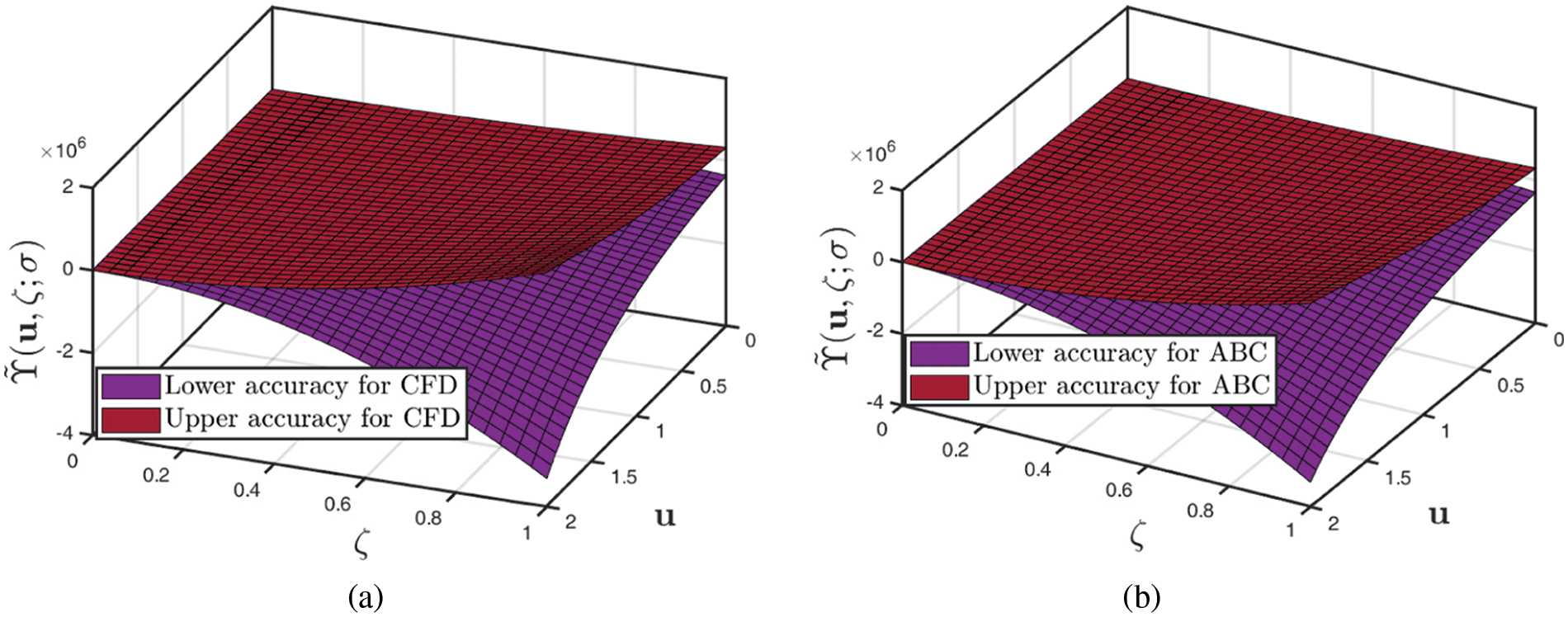
Figure 1: Analysis of 3D plots of Example 1 provided by (a) fuzzified CFD (b) fuzzified ABCFD technique when and fuzzy number lies in

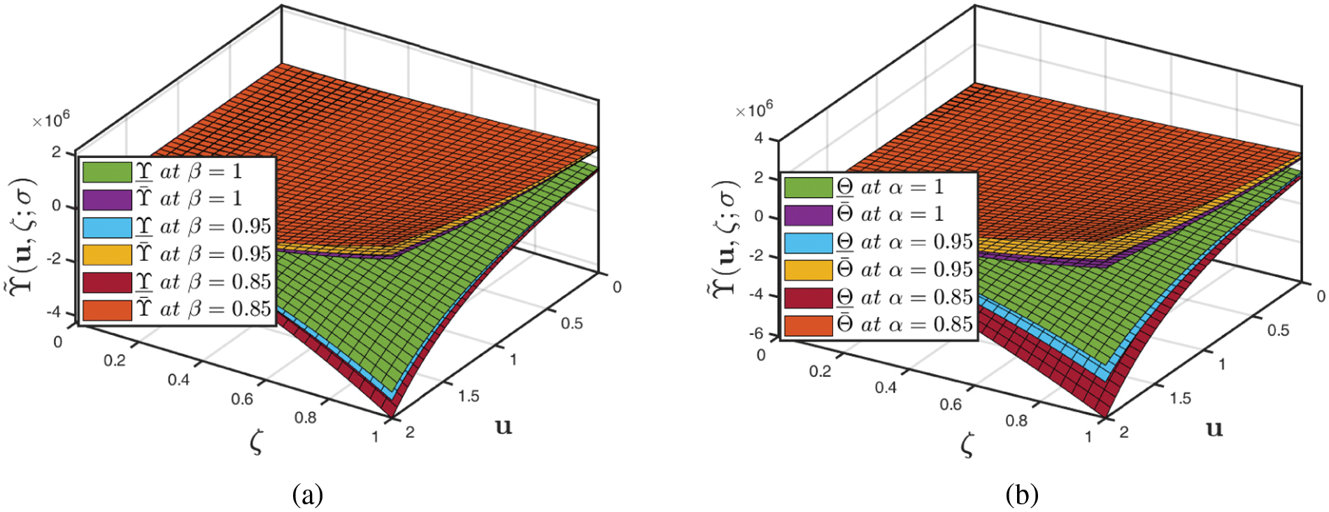
Figure 2: Analysis of several 3D profiles of Example 1 provided by (a) fuzzified CFD (b) fuzzified ABCFD techniques when fractional-order varies and fuzzy number lies in

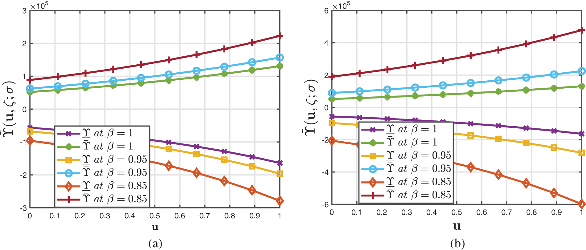
Figure 3: Analysis of several 2D profiles of Example 1 provided by (a) fuzzified CFD (b) fuzzified ABCFD techniques when fractional-order varies and fuzzy number lies in

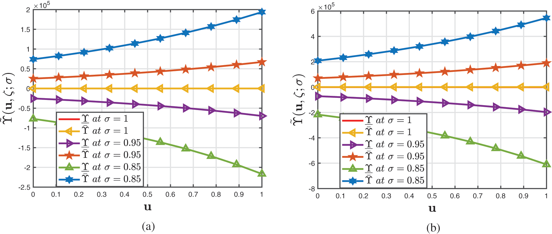
Figure 4: Analysis of several 2D profiles of Example 1 provided by (a) fuzzified CFD (b) fuzzified ABCFD techniques when ambiguity parameter varies and fractional-order

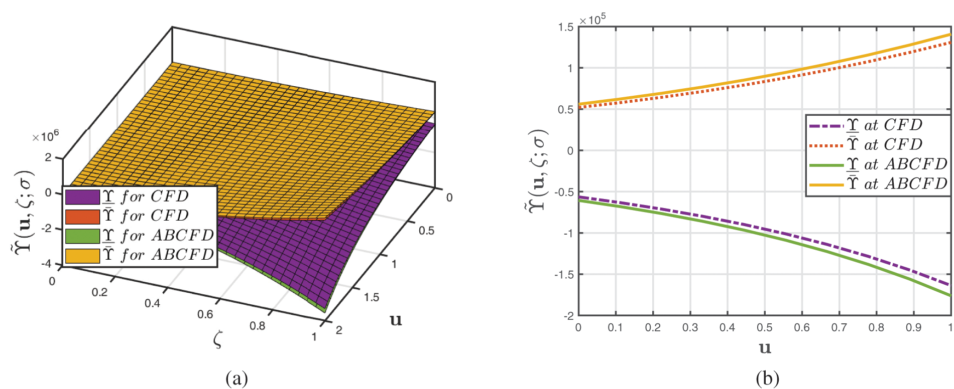
Figure 5: Analysis of several 3D and 2D profiles of Example 1 provided by fuzzified CFD and ABCFD techniques when ambiguity parameter and

The major aspect is that the AADM has supplied a couple of solutions for the BSe, one of the best-known frameworks in groundwater resources in terms of mathematical complexity and intensity. Whenever the formulae in these strategies take on a special significance, they can be employed to classify relatively new structures of evapotranspiration contours, irrigation and external phenomena.

4.2 Generalized Fuzzy FBSQe in

Example 2. Surmise that the general one-dimensional fuzzified FBSQe is denoted by

(42)

supplemented with fuzzified ICs

(43)

where for is fuzzy number.

The parametric extension of (42) is shown as

Case I. To begin, we implement the Aboodh transform to the initial part of (44) along with -differentiability under the CFD formula. Considering the Aboodh transform of the first foregoing scenario of (44), we have

Considering (44), we have

or likewise, we have

(44)

The solution to the unidentified sequence is written as

(45)

and the nonlinear components dealt by

(46)

where and are widely recognized Adomian polynomials that can be evaluated by the scheme (28).

Inserting (45) and (46) into (44), yields the following expression:

(47)

Implementing the inverse Aboodh transform and comparing expressions on both sides of (46), we determine the aforementioned recursive expressions by fuzzified CFD as follows:

As a consequence, the intended approximation is composed as

indicates that

Case II. To begin, we apply the Aboodh transform to the first part of (44) as well as -differentiability using the ABCFD formula.

Considering the Aboodh transform of the first foregoing scenario of (44), we have

or likewise, we get

(48)

The solution to the unidentified sequence is written as

(49)

and the nonlinear components are dealt by

(50)

where and are the widely recognized Adomian polynomials that can be evaluated by the scheme (28).

Inserting (47) and (50) into (48), then we have

(51)

Implementing the inverse Aboodh transform and comparing the expressions on both sides of (51), we determine the aforementioned recursive expressions by fuzzified ABCFD as follows:

As a consequence, the intended approximation is composed as

implies that

•   Fig. 6 depicts a 3D correlation of the coupled solutions of for Example 2 when and ambiguity component using -differentiability of CFD and ABCFD operators supplemented with fuzzified initial settings when real parameters are and The AADM solution is highly correlated, including both fractional operators.

•   Evaluation of diverse structural graphs for various fractional orders with the fuzzified CFD and ABCFD techniques is shown in Fig. 7. Furthermore, it can be demonstrated that by expanding the accurate depiction of hydrological cycle and aquifer complexities on steep topography in the fluid at .

•   The correlation of the coupled precision between the fuzzified CFD and ABCFD techniques for various fractional-orders, so if for spreading aquifer characterizations at hydrologic levels is shown in Fig. 8.

•   Fig. 9 depicts the 2D correlation of the upper accuracy and reliability of the fuzzified CFD and ABCFD techniques when . This simplifies the process of exploring the spatiotemporal connections between surface geomorphology and aquifer threshold.

•   Fig. 10 depicts the interfacial and 2D correlation by fuzzified CFD and ABCFD techniques that demonstrate the communications between the rain and evaporation procedures.

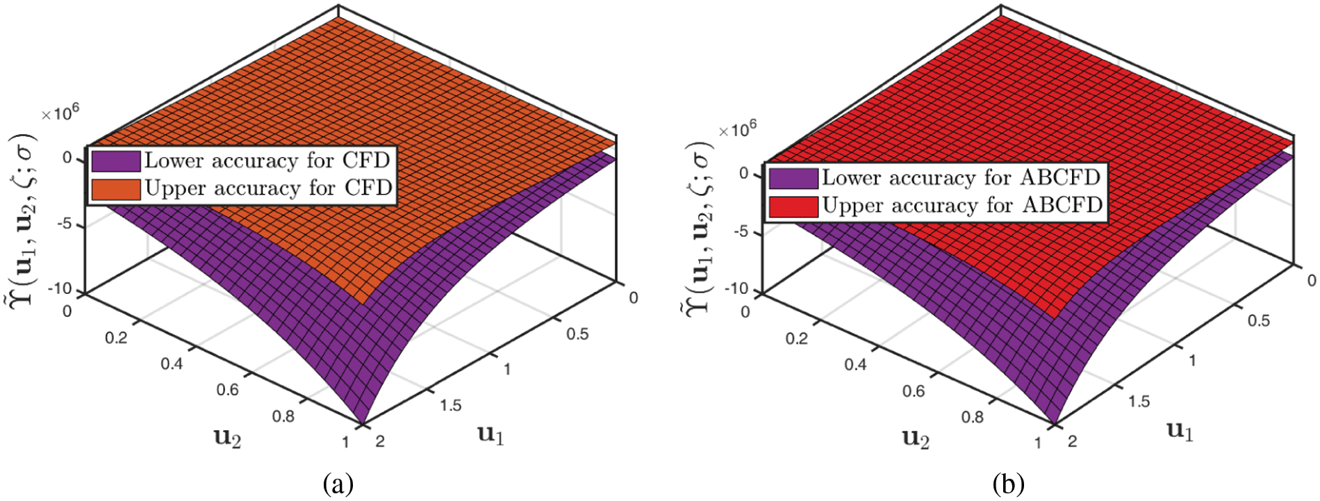
Figure 6: Analysis of 3D plots of Example 2 provided by (a) fuzzified CFD (b) Fuzzified ABCFD technique when and fuzzy number lies in

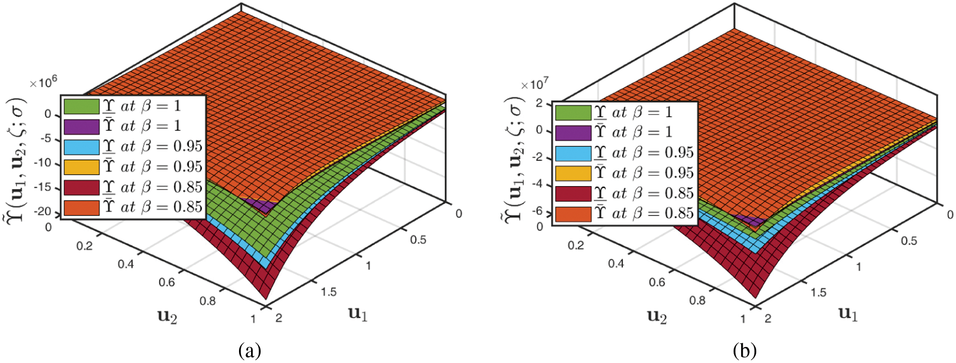
Figure 7: Analysis of several 3D profiles of Example 2 provided by (a) fuzzified CFD (b) fuzzified ABCFD techniques when fractional-order varies and fuzzy number lies in

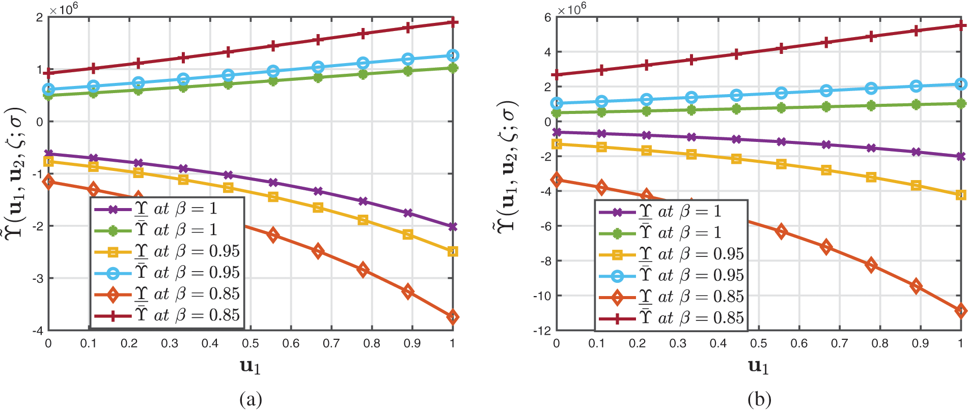
Figure 8: Analysis of several 2D profiles of Example 2 provided by (a) fuzzified CFD (b) fuzzified ABCFD techniques when ambiguity parameter varies and fractional-order

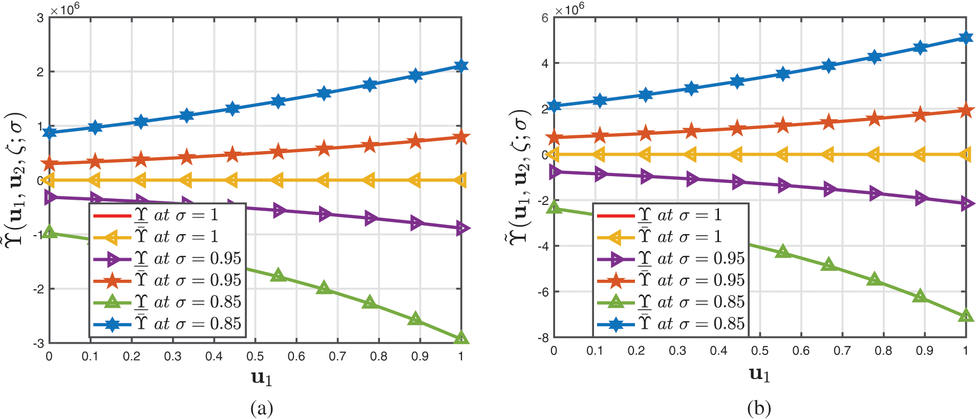
Figure 9: Analysis of several 2D profiles of Example 2 provided by (a) fuzzified CFD (b) fuzzified ABCFD techniques when ambiguity parameter varies and fractional-order

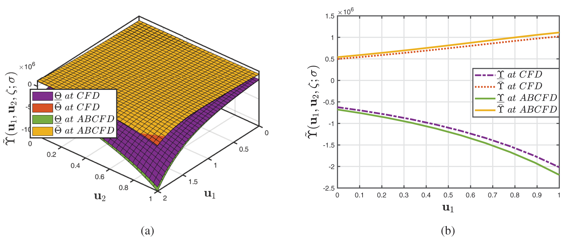
Figure 10: Analysis of several 3D and 2D profiles of Example 2 provided by fuzzified CFD and ABCFD techniques when ambiguity parameter and

The key point is that AADM has furnished combinations of solutions for the FBSQe, being one of the most effective configurations in groundwater with low processing complexity and intensity. Whenever the elements in these solutions carry a specific meaning, they can be employed to identify completely new frameworks of hydrology graphs, fertigation, and physical phenomena.

4.3 ()-Order Fuzzy FBSQe in

Example 3. Surmise that the general one-dimensional ()-order fuzzfied FBSQe is described as

(52)

supplemented with fuzzified ICs

(53)

where for is fuzzy number.

The parametric extension of (52) is shown as

(54)

Case I. To begin, we implement the Aboodh transform to the initial part of (54) along with differentiability under the CFD formula.

Considering the Aboodh transform of the first foregoing scenario of (54), we have

Considering (54), we have

or likewise, we have

(55)

The solutions to the unidentified sequence is written as

(56)

and the nonlinear components dealt by

(57)

where and are the widely recognized Adomian polynomials that can be evaluated by the scheme (28).

Inserting (56) and (57) into (55), yields the following expression:

(58)

Implementing the inverse Aboodh transform and comparing expressions on both sides of (58), we determine the aforementioned recursive expressions by fuzzified CFD as follows:

(59)

As a consequence, the intended approximation is composed as

indicates that

Case II. To begin, we apply the Aboodh transform to the first part of (33), as well as -differentiability using the ABCFD formula.

Considering the Aboodh transform of the first foregoing scenario of (33), we have

or likewise, we have

(60)

The solution to the unidentified sequence is written as

(61)

and the nonlinear components are dealt by

(62)

where and are the widely recognized Adomian polynomials that can be evaluated by the scheme (28).

Inserting (61) and (62) into (60), yields the following expression:

(63)

Implementing the outlined in the preceding inverse Aboodh transform and then comparing considerations on both sides of the aforementioned Eq. (63), we determine the respective recursive expressions by the fuzzified ABCFD operator. Therefore, with the assistance of these derivative features:

As a consequence, the intended approximation is composed as

indicates that

Now, perform a two-way analysis of variance on these documentation and examine whether there is a massive distinction between AADM’s ABCFD and CFD solutions.

(i) We develop the two null hypotheses that correlate to the challenges that

(a) there is no significant difference between the ABCFD data,

and

(b) there is no significant difference between the ABCFD data, as

(64)

(ii) The corresponding alternative hypothesis would be

(65)

(iii) The test-statistics to utilized with the level of significance is is defined as

(66)

which have -distribution having degree of freedoms and and respectively, when the null hypotheses are true.

(iv) The critical regions are

(v) Since the computed value of does not fall in the critical region but the calculated value of falls in the critical region, we accept the hypothesis relating to the ABCFD and reject the hypotheses corresponding to the fact that there is no significant difference between CFD data.

•   The comparative assessment of coupled results calculated by employing the fuzzified CFD, ABCFD technique, and Xu’s optimization technique is shown in Table 1. In addition, Tables 2 and 3 displays the comparison evaluation for the CFD and ABCFD techniques corresponding with the AADM and the outcomes supplied by [49]. All our findings indicate that our conclusions are concise and valid.

•   Fig. 11a depicts a 3D analysis of the coupled solutions of for Example 3 when and ambiguity parameter using -differentiability of CFD and ABCFD supplemented to fuzzified ICs even before real parameters are and All fractional operators have a straightforward connection to the AADM solution.

•   The distinction of various structural graphs for distinct fractional-orders to the fuzzified CFD and ABCFD techniques is shown in Figs. 12a and 12b. Furthermore, at , improving the accuracy of watershed and aquifer interactions on mountainsides can be demonstrated.

•   The correlation of the coupled accuracies between the fuzzified CFD and ABCFD techniques for various fractional-orders when for diversifying streamflow profiles at flood risk levels is shown in Fig. 13.

•   Fig. 14 depicts the 2D correlation of the upper precision of the fuzzified CFD and ABCFD techniques when . This enables it to study the spatiotemporal features between subsurface topography and aquifer threshold.

•   The horizon and 2D comparisons by the fuzzified CFD and ABCFD techniques that exhibit the connections between the snowfall and groundwater methodology are illustrated in Fig. 15.

•   The key point is that AADM has furnished a couple of findings for the FBSQe, among which the tendencies for effective models in groundwater, to low processing complexity and density. Whenever the parameters in these strategies take on a special significance, they may be employed to identify completely new frameworks of rainfall-runoff peaks, drainage systems, and physical phenomena.

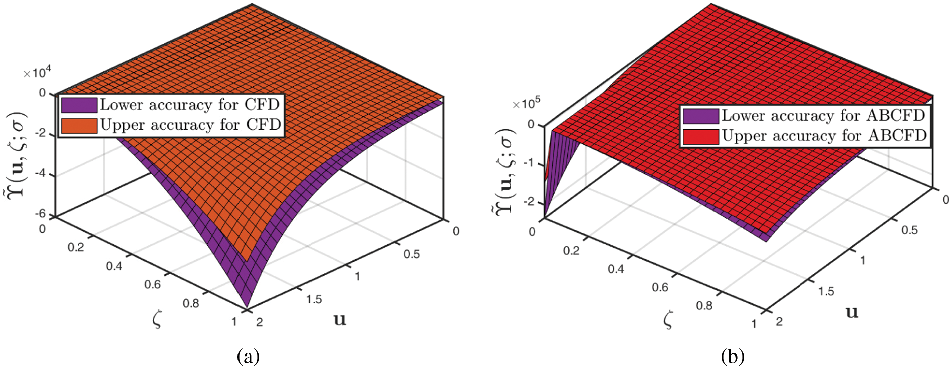
Figure 11: Analysis of 3D plots of Example 3 provided by (a) fuzzified CFD (b) fuzzified ABCFD technique when and fuzzy number lies in

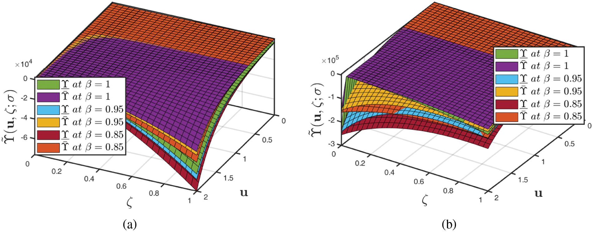
Figure 12: Analysis of several 3D profiles of Example 3 provided by (a) fuzzified CFD (b) fuzzified ABCFD techniques when fractional-order varies and fuzzy number lies in

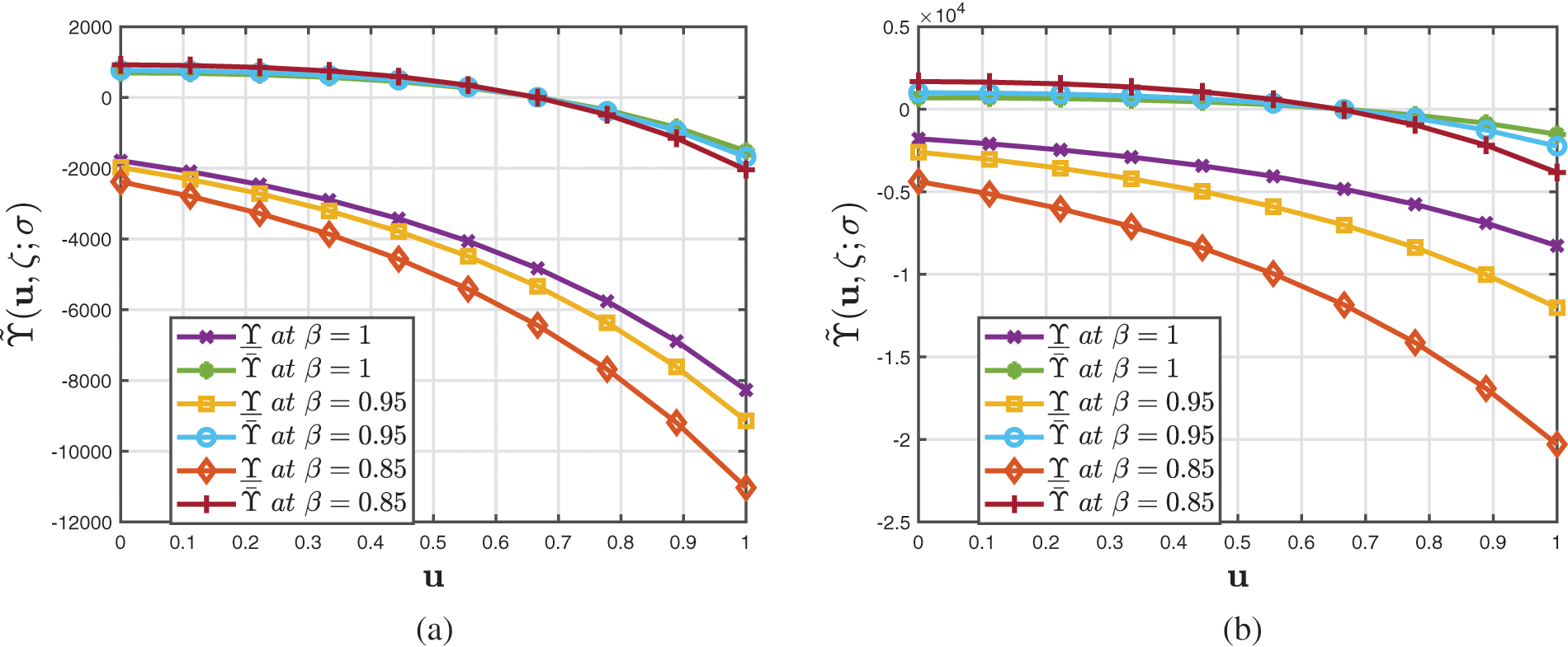
Figure 13: Analysis of several 2D profiles of Example 3 provided by (a) fuzzified CFD (b) fuzzified ABCFD techniques when ambiguity parameter varies and fractional-order

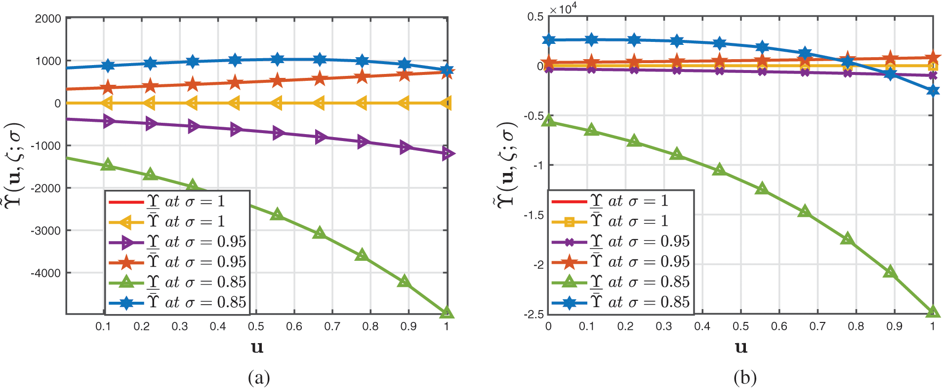
Figure 14: Analysis of several 2D profiles of Example 3 provided by (a) fuzzified CFD (b) fuzzified ABCFD techniques when ambiguity parameter varies and fractional-order

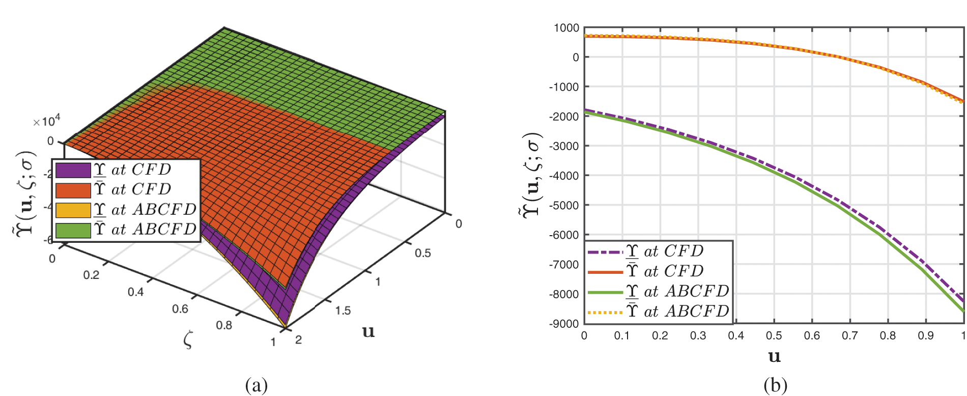
Figure 15: Analysis of several 3D and 2D profiles of Example 3 provided by fuzzified CFD and ABCFD techniques when ambiguity parameter and

5  Conclusion

This relatively new family of results enables the exploration and advancement of geothermal regimens using FBSE in accordance with the fuzzy concept. While other techniques are influenced by in some ways, the findings presented here explicitly rely on the control point. This produces an extremely constructive system for analyzing intricate components, including enchantment formulation and aquifer topography. Understanding how to categorize the interconnection in both the Aboodh transform and the analytical schema (ADM) simplifies the investigation of ambiguous fractional formulations. These observations were developed using a sophisticated technique. The features and drawbacks of the provided techniques are discussed. The outcomes go into greater detail about the commonalities and discrepancies between the two fuzzified fractional formulation techniques. The AADM technique is advantageous for significantly bringing down computation overhead. The AADM, on the other hand, has a privilege compared to other analytical simulations because it avoids the application of the Lagrange multiplier, stationary requirements, and complex formulae that are extremely noisy. The suggested technique has an additional advantage over the wavelet transform in terms of its entitlements. To avoid adjusting the research hypotheses after the outcomes are known, a statistical experiment is carried out between the research results of both fractional derivatives. This indicates that the findings of ABCFD are more reliable than the CFD technique. Furthermore, because ripples have a major influence on ecological concerns as well as oceanfront coasts and underwater, the discussed observations facilitate comprehensive and pragmatic investigations into the essence of these shock waves, which can be utilized to cultivate weather forecasting trend scenarios.

Funding Statement: The authors received no specific funding for this study.

Conflicts of Interest: The authors declare that they have no conflicts of interest to report regarding the present study.

References

1. Xu, L., Auston, D. H., Hasegawa, A. (1992). Propagation of electromagnetic solitary waves in dispersive nonlinear dielectrics. Physical Review A, 45(5), 3184–3193. https://doi.org/10.1103/PhysRevA.45.3184 [Google Scholar] [PubMed] [CrossRef]

2. Karpman, V. I. (1975). Nonlinear waves in dispersive media. Oxford New York: Pergamon Press. https://doi.org/10.1016/C2013-0-05645-9 [Google Scholar] [CrossRef]

3. Turisyn, S. K., Falkovich, G. E. (1985). Stability of magnetoelastic solitons and self-focusing of sound in antiferromagnetics. Soviet Physics-JETP, 62(1), 146–152. https://doi.org/10.0038-5646/85/070146-0704.0 [Google Scholar] [CrossRef]

4. Ablowitz, M. J., Clarkson, P. A. (1991). Solitons, non-linear evolution equations and inverse scattering transform. Cambridge: Cambridge University Press. https://doi.org/10.1017/CBO9780511623998 [Google Scholar] [CrossRef]

5. Islama, R., Khan, K., Ali Akbar, M., Islama, M. E., Ahmed, M. T. (2015). On traveling wave solutions of some nonlinear evolution equations. Alexandria Engineering Journal, 54(2), 263–269. https://doi.org/10.1016/j.aej.2015.01.002 [Google Scholar] [CrossRef]

6. Wazwaz, A. M. (2004). A sine-cosine method for handling nonlinear wave equations. Mathematical and Computer Modelling, 40, 499–508. https://doi.org/10.1016/j.mcm.2003.12.010 [Google Scholar] [CrossRef]

7. Chow, K. W. (1995). A class of exact periodic solutions of nonlinear envelope equation. Journal of Mathematical Physics, 36(8), 4125–4137. https://doi.org/10.1063/1.530951 [Google Scholar] [CrossRef]

8. Malflieta, W., Hereman, W. (1996). The tanh method: Exact solutions of nonlinear evolution and wave equations. Physica Scripta, 54(6), 563–568. https://doi.org/10.1088/0031-8949/54/6/003 [Google Scholar] [CrossRef]

9. Zhang, J. L., Wang, M. L., Wang, Y. M., Fang, Z. D. (2006). The improved F-expansion method and its applications. Physics Letters A, 350, 103–109. https://doi.org/10.1016/j.physleta.2005.10.099 [Google Scholar] [CrossRef]

10. Hirota, R. (1973). Exact envelope soliton solutions of a nonlinear wave equation. Journal of Mathematical Physics, 14(7), 805–810. https://doi.org/10.1063/1.1666399 [Google Scholar] [CrossRef]

11. Shahida, N., Tunc, C. (2019). Resolution of coincident factors in altering the flow dynamics of an MHD elastoviscous fluid past an unbounded upright channel. Journal of Taibah University for Science, 13(1), 1022–1034. https://doi.org/10.1080/16583655.2019.1678897 [Google Scholar] [CrossRef]

12. Alharbi, A. R., Almatrafi, M. B., Abdelrahman, M. A. E. (2019). The extended Jacobian elliptic function expansion approach to the generalized fifth order KdV equation. Journal of Physics A: Mathematical and Theoretical Institute of Physics, 10(4), 310. [Google Scholar]

13. Alharbi, A. R., Almatrafi, M. B. (2020). Numerical investigation of the dispersive long wave equation using an adaptive moving mesh method and its stability. Results in Physics, 16(9), 102870. https://doi.org/10.1016/j.rinp.2019.102870 [Google Scholar] [CrossRef]

14. Bear, J. (1979). Hydraulic of groundwater. New York: McGraw Hill Book Company. [Google Scholar]

15. Akbar, M. A., Akinyemi, L., Yao, S. W., Jhangeer, A., Rezazadeh, H. et al. (2021). Soliton solutions to the Boussinesq equation through sine-Gordon method and Kudryashov method. Results in Physics, 25, 104228. https://doi.org/10.1016/j.rinp.2021.104228 [Google Scholar] [CrossRef]

16. Ma, Y. L., Li, B. Q. (2022). Bifurcation solitons and breathers for the nonlocal Boussinesq equations. Applied Mathematical Letters, 124(2), 107677. https://doi.org/10.1016/j.aml.2021.107677 [Google Scholar] [CrossRef]

17. Li, B. Q., Wazwaz, A. M., Ma, Y. L. (2022). Two new types of nonlocal Boussinesq equations in water waves: Bright and dark soliton solutions. Chinese Journal of Physics, 77(2), 1782–1788. [Google Scholar]

18. Mehdinejadiani, B., Jafari, H., Baleanu, D. (2013). Derivation of a fractional Boussinesq equation for modelling unconfined groundwater. The European Physical Journal Special Topics, 222(8), 1805–1812. https://doi.org/10.1140/epjst/e2013-01965-1 [Google Scholar] [CrossRef]

19. El-Wakil, S. A., Abulwafa, E. M. (2015). Formulation and solution of space-time fractional Boussinesq equation. Nonlinear Dynamics, 80, 167–175. https://doi.org/10.1007/s11071-014-1858-3 [Google Scholar] [CrossRef]

20. Zhuang, P., Liu, F., Turner, I., Gu, Y. T. (2014). Finite volume and finite element methods for solving a one-dimensional space-fractional Boussinesq equation. Applied Mathematical Modelling, 38, 3860–3870. https://doi.org/10.1016/j.apm.2013.10.008 [Google Scholar] [CrossRef]

21. Abassy, T. A., El-Tawil, M. A., El-Zoheiry, H. (2007). Modified variational iteration method for Boussinesq equation. Computers & Mathematics with Applications, 54, 955–965. https://doi.org/10.1016/j.camwa.2006.12.040 [Google Scholar] [CrossRef]

22. Wu, M. C., Hsieh, P. C. (2019). Improved solutions to the linearized Boussinesq equation with temporally varied rainfall recharge for a sloping aquifer. Water, 11(4), 826. https://doi.org/10.3390/w11040826 [Google Scholar] [CrossRef]

23. Chang, S. S. L., Zadeh, L. (1972). On fuzzy mapping and control. IEEE Transactions on Systems, Man, and Cybernetics, 2(1), 30–34. https://doi.org/10.1109/TSMC.1972.5408553 [Google Scholar] [CrossRef]

24. Atangana, A., Baleanu, D. (2016). New fractional derivatives with nonlocal and nonsingular kernel, theory and application to heat transfer model. Journal of Thermal Science, 20(2), 763–769. https://doi.org/10.2298/TSCI160111018A [Google Scholar] [CrossRef]

25. Rashid, S., Abouelmagd, E. I., Khalid, A., Farooq, F. B., Chu, Y. M. (2022). Some recent developments on dynamical h-discrete fractional type inequalities in the frame of nonsingular and nonlocal kernels. Fractals, 30, 2240110. https://doi.org/10.1142/S0218348X22401107 [Google Scholar] [CrossRef]

26. Podlubny, I. (1998). Fractional differential equations, vol. 1998. San Diego, CA: Lightning Source Inc., Academic Press. [Google Scholar]

27. Atangana, A., Qureshi, S. (2019). Modeling attractors of chaotic dynamical systems with fractal-fractional operators. Chaos Solitons & Fractals, 123(3), 320–337. https://doi.org/10.1016/j.chaos.2019.04.020 [Google Scholar] [CrossRef]

28. Arqub, O. A., Al-Smadi, M., Momani, S., Hayat, T. (2017). Application of reproducing kernel algorithm for solving second-order, two-point fuzzy boundary value problems. Soft Computing, 21(23), 7191–7206. https://doi.org/10.1007/s00500-016-2262-3 [Google Scholar] [CrossRef]

29. Arqub, O. A. (2017). Adaptation of reproducing kernel algorithm for solving fuzzy Fredholm–Volterra integrodifferential equations. Neural Computing and Applications, 28(7), 15911610. https://doi.org/10.1007/s00521-015-2110-x [Google Scholar] [CrossRef]

30. Rashid, S., Jarad, F., Abualnaja, K. M. (2021). On fuzzy Volterra-Fredholm integrodifferential equation associated with Hilfer-generalized proportional fractional derivative. AIMS Mathematics, 6(10), 10920–10946. https://doi.org/10.3934/math.2021635 [Google Scholar] [CrossRef]

31. Agarwal, R. P., Arshad, S., O’Regan, D., Lupulescu, V. (2012). Fuzzy fractional integral equations under compactness type condition. Fractional Calculus and Applied Analysis, 15(4), 572–590. https://doi.org/10.2478/s13540-012-0040-1 [Google Scholar] [CrossRef]

32. Bede, B., Stefanini, L. (2013). Generalized differentiability of fuzzy-valued functions. Fuzzy Sets and Systems, 230, 119–141. https://doi.org/10.1016/j.fss.2012.10.003 [Google Scholar] [CrossRef]

33. Alikhani, R., Bahrami, F. (2017). Global solutions for nonlinear fuzzy fractional integral and integrodifferential equations. Communications in Nonlinear Science and Numerical Simulations, 18(8), 2007–2017. https://doi.org/10.1016/j.cnsns.2012.12.026 [Google Scholar] [CrossRef]

34. Allahviranloo, T., Salahshour, S., Abbasbandy, S. (2012). Explicit solutions of fractional differential equations with uncertainty. Soft Computing, 16(2), 297–302. [Google Scholar]

35. Allahviranloo, T., Kermani, A. M. (2010). Numerical methods for fuzzy partial differential equations under new definition for derivative. International Journal of Fuzzy Systems, 7, 33–50. [Google Scholar]

36. Arqub, O. A., Al-Smadi, M., Momani, S., Hayat, T. (2017). Application of reproducing kernel algorithm for solving second-order, two-point fuzzy boundary value problems. Soft Computing, 21(23), 7191–7206. https://doi.org/10.1007/s00500-016-2262-3 [Google Scholar] [CrossRef]

37. Zhao, T. H., Castillo, O., Jahanshahi, H., Yusuf, A., Alassafi, M. O. et al. (2021). A fuzzybased strategy to suppress the novel coronavirus (2019-NCOV) massive outbreak. Applied and Computational Mathematics, 20, 160–176. [Google Scholar]

38. Adomian, G. (1988). A review of the decomposition method in applied mathematics. Journal of Mathematical Analysis and Applications, 135(2), 501–544. https://doi.org/10.1016/0022-247X(88)90170-9 [Google Scholar] [CrossRef]

39. Rashid, S., Ashraf, R., Bonyah, E. (2022). On analytical solution of time-fractional biological population model by means of generalized integral transform with their uniqueness and convergence analysis. Journal of Function Spaces, 2022(4), 7021288. https://doi.org/10.1155/2022/7021288 [Google Scholar] [CrossRef]

40. Rashid, S., Ashraf, R., Bayones, F. S. (2021). A novel treatment of fuzzy fractional Swift-Hohenberg equation for a hybrid transform within the fractional derivative operator. Fractal and Fractional, 5(4), 209. https://doi.org/10.3390/fractalfract5040209 [Google Scholar] [CrossRef]

41. Zimmermann, H. (1991). Fuzzy set theory and its applications. Dordrecht: Kluwer Academic Publishers. [Google Scholar]

42. Zadeh, L. A. (1965). Fuzzy sets. Information and Control, 8(3), 338–353. https://doi.org/10.1016/S0019-9958(65)90241-X [Google Scholar] [CrossRef]

43. Allahviranloo, T. (2021). Fuzzy fractional differential operators and equation studies in fuzziness and soft computing. Berlin: Springer. [Google Scholar]

44. Salahshour, S., Ahmadian, A., Senu, A., Baleanu, D., Agarwal, P. P. (2015). On analytical aolutions of the fractional differential equation with uncertainty: Application to the Basset problem. Entropy, 17(2), 885–902. https://doi.org/10.3390/e17020885 [Google Scholar] [CrossRef]

45. Allahviranloo, T., Ahmadi, M. B. (2010). Fuzzy Lapalce transform. Soft Computing, 14(3), 235–243. https://doi.org/10.1007/s00500-008-0397-6 [Google Scholar] [CrossRef]

46. Aboodh, K. S. (2013). The new integral transform Aboodh transform. Global Journal of Pure and Applied Mathematics, 9, 35–43. [Google Scholar]

47. Salahshour, S., Allahviranloo, T., Abbasbandy, S. (2012). Solving fuzzy fractional differential equations by fuzzy Laplace transforms. Communications in Nonlinear Science and Numerical Simulation, 17(3), 1372–1381. https://doi.org/10.1016/j.cnsns.2011.07.005 [Google Scholar] [CrossRef]

48. Awuya, M. A., Subasi, D. (2021). Aboodh transform iterative method for solving fractional partial differential equation with Mittag-Leffler kernel. Symmetry, 13(11), 2055. https://doi.org/10.3390/sym13112055 [Google Scholar] [CrossRef]

49. Xu, F., Gao, Y. X., Zhang, W. (2015). Construction of analytic solution for time-fractional Boussinesq equation using iterative method. Advances in Mathematical Physics, 2015, 1–7. https://doi.org/10.1155/2015/506140 [Google Scholar] [CrossRef]