Open-Source Codes of Topology Optimization: A Summary for Beginners to Start Their Research

1  Introduction

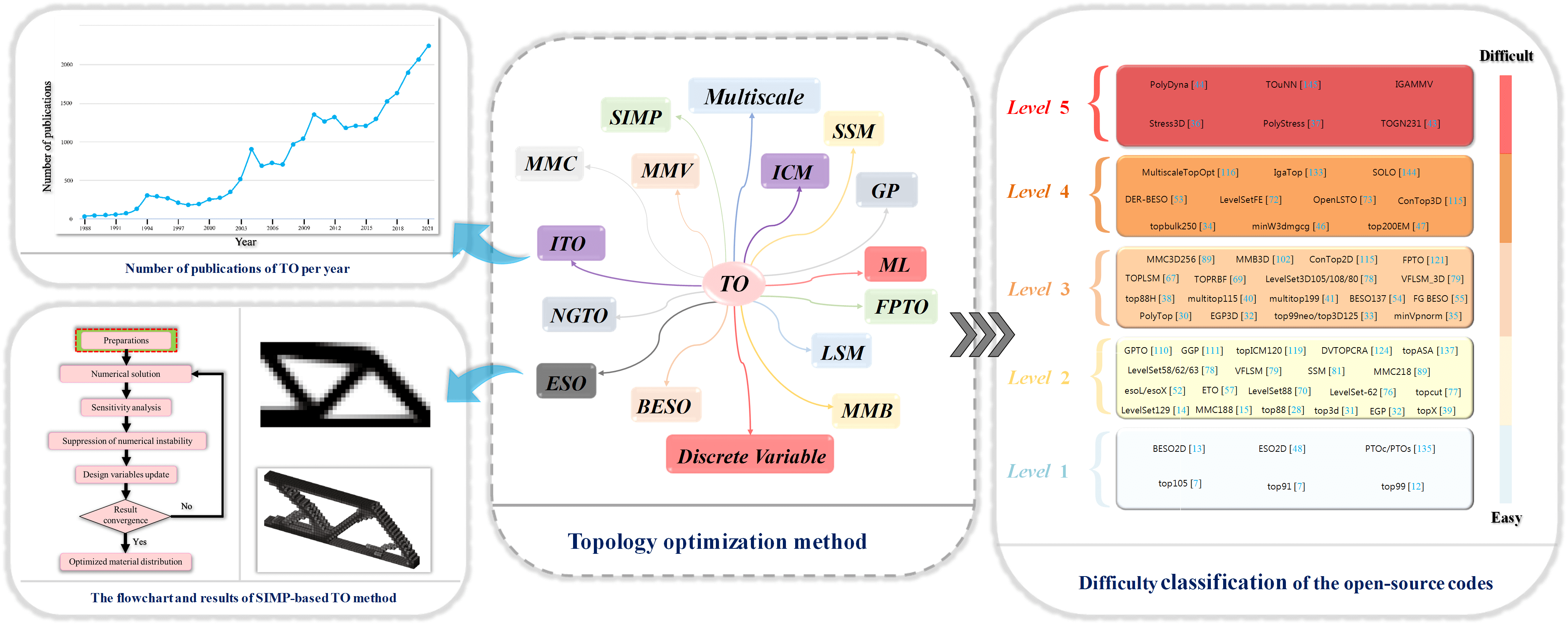
Topology optimization (TO) is one of the most intelligent structural design methods, intending to automatically find the optimal structure in a design domain according to given loads and constraints. The first paper about TO dates back to the work of Michell [1] in 1904, where a solution method of classical Michell truss structures was derived. Prager et al. [2,3] extended Michell’s theory to grillages and their layout optimizations. The early work focused on the optimization theory by analytical methods, which was limited to simple cases. The first general numerical TO method was proposed by Cheng and Olhoff on the optimal design of solid elastic plates [4], and after the milestone work of Bendsøe et al. [5] by introducing a homogenization approach to TO, numerical TO methods have been widely investigated, such as solid isotropic material with penalization (SIMP) [6,7], evolutionary structural optimization (ESO) [8,9], and level-set based topology optimization [10,11].

Fig. 1 shows the number of publications of TO per year from 1988 (the year Bendsøe et al. published the milestone work [5]) to 2021, where it can be found that the research in TO has been growing, particularly after 2000. One of the most important reasons for the rapid growth of TO research is the seminal paper providing the first open-source TO Matlab code (top99) in 2001 [12], and this code is still one of the best tutorials for beginners to learn TO. Since then, plenty of publications, especially on new TO methodology, have provided open-source codes with them, which greatly promote TO research. For example, Huang et al. [13] provided a bi-directional evolutionary structural optimization (BESO) Matlab code (BESO2D) in their book on the evolutionary topology optimization of continuum structures. Challis presented a 129-line Matlab code (LevelSet129) of discrete level-set TO in [14]. Zhang et al. [15] gave a 188-line Matlab code (MMC188) of TO using the moving morphable components (MMC) method, which helps readers easier to understand the essential features of the new approach. Besides, some researchers choose to publish their open-source codes on their group/personal websites or public web hosting, e.g., the TopOpt group at https://www.topopt.mek.dtu.dk, Paulino’s group at https://paulino.ce.gatech.edu, and the open-source code for level set TO at github: https://github.com/M2DOLab/OpenLSTO-lite, and in this way the codes can be distributed immediately.

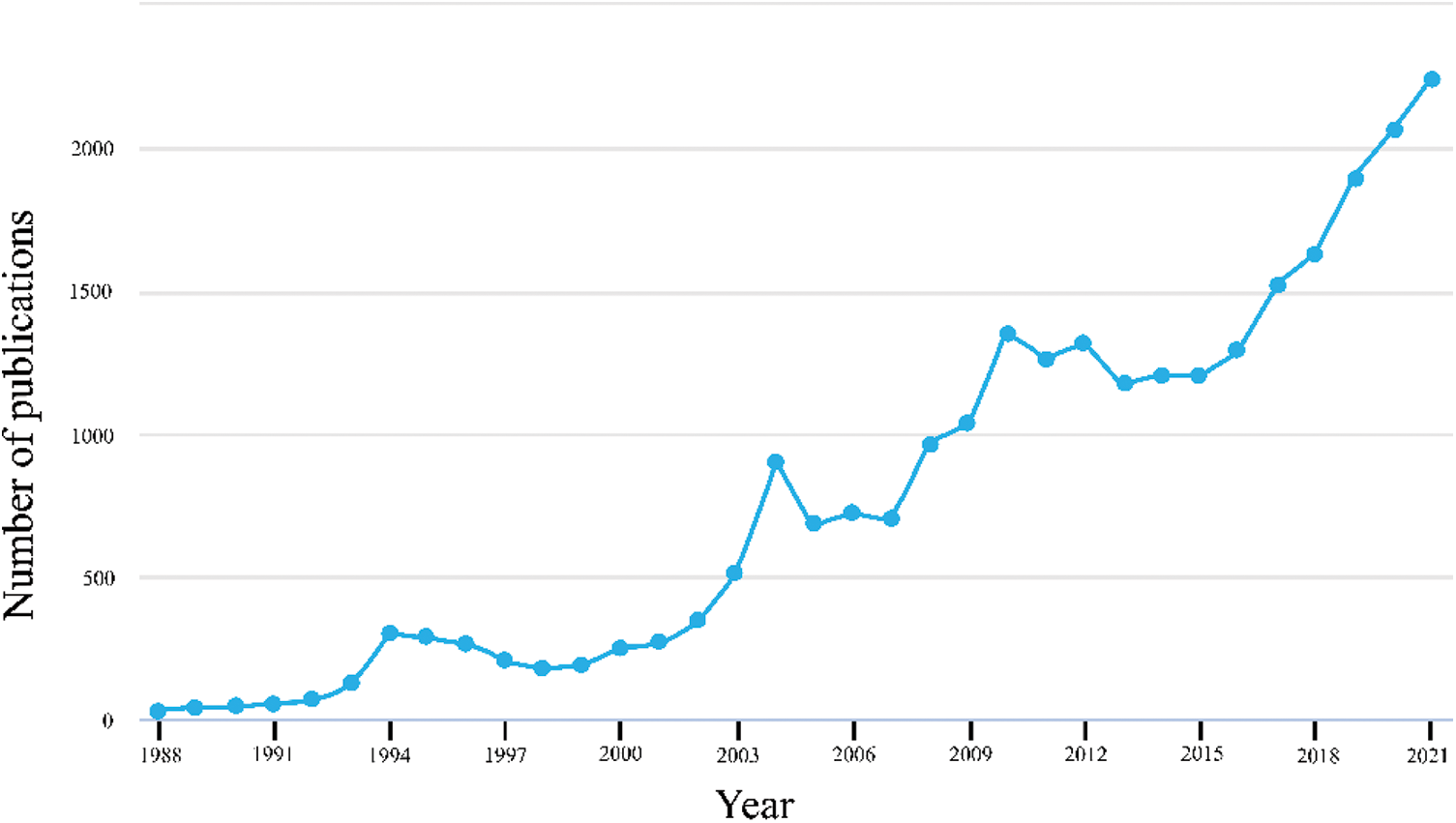
Figure 1: Number of publications of topology optimization per year (data from Scopus)

An open-source code presents the implementation of a method in detail, which is of great value to readers interested in that method and able to attract more people to use and extend the method. However, with more and more open-source codes provided by researchers, it will take quite a long time to find the one they need, especially for people who are unfamiliar with the research field. For TO, there are excellent review papers that summarize the existing literature on a topic to help people understand the research of that topic [16–21], particularly a recent review of educational articles [22]. Still, all of them are full of professional knowledge that makes it difficult for beginners to quickly grasp the details of various types of TO.

In this paper, we intend to provide a summary of the open-source codes of TO from the classical 99-line Matlab code of Sigmund [12] proposed in 2001, and we hope this summary can make it easier for newcomers to start their research on TO. An outline of the remainder of this paper is summarized as follows: Section 2 introduces the basic concept of TO. Section 3 presents a review of open-source TO codes based on SIMP. Section 4 gives a review of open-source TO codes using evolutionary methods. Section 5 discusses open-source codes of level set TO. Section 6 summarises open-source codes of a new type of TO based on explicit geometries respectively. Section 7 reviews the open-source codes of multiscale TO. Section 8 introduces some other TOs and their applications. Finally, the conclusions are given in Section 9.

2  Basic Concept of TO

The objective of TO is to determine the optimal material distribution within a design domain according to specified loads and constraints. One of the typical TO problems is the compliance minimization problem:

Min :C(x)=UTKUSubject to :KU=F∑i=1NVixi−V∗≤0xmin≤xi≤1(1)

where C is the objective function (i.e., compliance), x is the design variable vector containing all design variable xi, K and U are the global stiffness matrix and the displacement vector, N represents the total number of design variables, Vi and V* are the volume corresponding to the ith design variable and the volume constraint of the design domain.

The most critical stage in TO is determining the gradient of the objective and constraint with respect to the design variables. For various TO methods, the design variables can be different. For example, the design variable xi denotes the density of the ith element in SIMP and ESO/BESO methods but denotes the level-set function of the ith node in the level-set based method. In general, the gradient can be used to update the design variables by a gradient-based algorithm such as sequential quadratic programming (SQP) [23], the optimality criteria (OC) method [24], and the method of moving asymptotes (MMA) [25]. However, when the gradient is too difficult to be obtained, non-gradient-based approaches such as genetic algorithm (GA) [26] and Grey wolf optimization (GWO) [27] to solve the optimization problem without the gradient but with lower efficiency than the gradient method.

3  SIMP TO

The SIMP TO is the most popular TO method, which has been effectively applied to a variety of issues. This section will introduce the basic theory, open-source codes and application fields.

3.1 Basic Theory of SIMP TO

The SIMP model is a typical density-stiffness interpolation model for TO problems, which improves and simplifies the homogenization process. During the optimization process, the intermediate densities are penalized by taking the power exponent p of the artificial material density, so that the density of the material tends to be as close to “0” or “1” as feasible.

The mathematical expression of the SIMP model is stated as follows:

E(ρi)=Emin+xip(E0−Emin)(2)

where E is the optimized elastic modulus; Emin and E0 represent the elastic modulus of the solid element and low-strength material element, respectively.

Since Emin << E0, Eq. (2) can be transformed into

E(ρi)=xipE0(3)

The element stiffness matrix ki is expressed as follows:

ki=E(xi)k∗=xipE0k∗=xipk0(4)

where k* is the element stiffness matrix obtained by separating elastic modulus from ki, and k0 is the elemental stiffness matrix of the solid material.

The compliance minimization continuum structure TO problem with the volume constraint can be described using the SIMP model as follows:

Find :x={x1,x2,…,xn}T∈ΩMin :C=FTU=UTKU=∑i=1nxipuiTk0uiSubject to : KU=F∑i=1NVixi−V∗≤0xmin≤xi≤1(5)

where ui is the displacement column vector of the material element.

Compared to the homogenization method, SIMP reduces the number of design variables and improves computational efficiency. Consequently, SIMP is easier to integrate with commercial finite element software. Currently, the majority of TO functions in existing commercial software are implemented using SIMP implementation.

The flowchart of SIMP-based TO method is shown in Fig. 2.

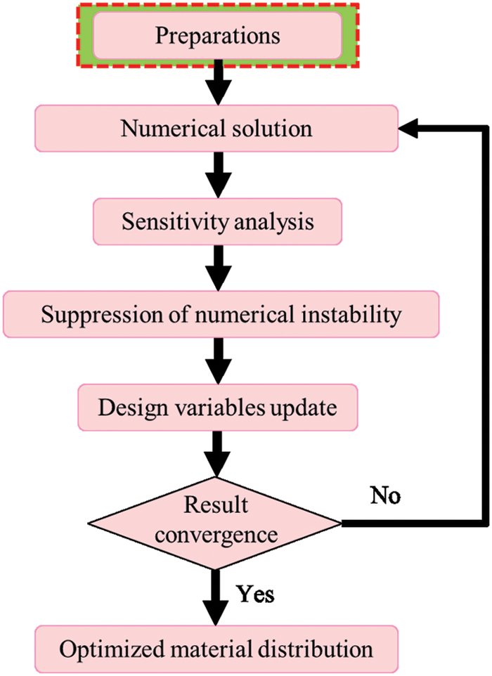
Figure 2: The flowchart of SIMP-based TO method

3.2 Basic Codes of SIMP TO

The fundamental codes of SIMP TO mainly cover 2D and 3D domains. In 2001, Sigmund [12] published the first educational 99-line Matlab code (top99) for compliance minimization with the stipulated material usage in the 2D structure. On top of that, Bendsøe et al. [7] extended a 105-line code (top105) for the compliance mechanism synthesis problem and a 91-line code (top91) for the heat conduction problem.

Ten years after the original, a more efficient and concise 88-line version code (top88) was released [28], with vectored form replacing the rather time-consuming loops. In addition, the density filter alternative implementations, such as the built-in Matlab function conv2 and the Helmholtz partial differential equation (PDE), are described. It is worth mentioning that, aiming to address the lack of the underlying theory and derivation under the works of the top99/88, Zhou et al. [29] presented a brief note for beginners to build a complete theoretical foundation without additional literature. Talischi et al. [30] published a MATLAB code for topology optimization in arbitrary domains using unstructured polygonal FE meshes called PolyTop. Liu et al. [31] provided 88-lines-inherited 3D code (top3d). The built-in function pcg representing the iterative solver is recommended to expedite the solution of large-scale linear equations. Compared to the earlier sources, Matlab codes (EGP and EGP3D) were provided by Zeng et al. [32] for TO of 2D and 3D structures utilizing a gradient projection-based approach. Meanwhile, Ferrari et al. [33] further developed new 2D (top99neo) and 3D (top3D125) MATLAB codes based on the top99 and presented a 250-line Matlab code (topbulk250) for linearized buckling criteria [34], the above codes jointly eliminate all the computational bottlenecks associated with setting up the buckling analysis and allow buckling TO problems of an interesting size to be solved on a laptop. Fig. 3 depicts the topological configurations of the cantilever beam in 2D and 3D.

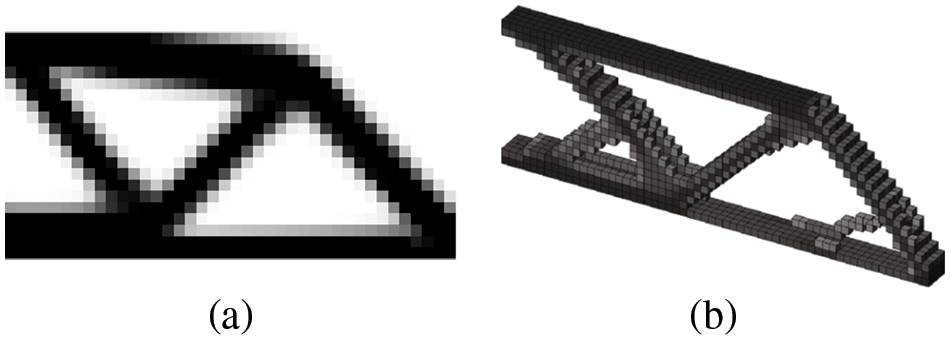
Figure 3: Topology optimization of a cantilever beam (a) 2D and (b) 3D [31]

3.3 Application Fields of SIMP

The primary advantage of SIMP over other optimization methods is its natural universality, and related research fields include stiffness, frequency, piezoelectricity, acoustics, optics, etc. In addition to the generally prevalent volume constraints, SIMP TO increasingly considers stress constraints. Amir [35] proposed a stress-constrained TO utilizing imprecise design sensitivity, i.e., an MGCG solver for the state and adjoint equations. The results demonstrated that the optimal solutions agreed with those produced by a precise solver, with significant iterations savings. The corresponding Matlab code (minVpnorm) for reproducing the results is hosted on the GitHub website https://github.com/odedamir/topopt-stress-inexact-sensitivities. Deng et al. [36] presented a 3D Matlab code (Stress3D) for the stress minimization tasks, which were validated by the finite difference approximation. Giraldo-Londoño et al. [37] have released PolyStress, a Matlab solution for TO with stress constraints at the local level. The augmented Lagrangian approach was adopted to address vast local stress constraints, avoiding conventional aggregation techniques.

Andreassen et al. [38] extended SIMP to TO of material design and offered an informative explanation of numerical homogenization in a Matlab code (top88H). The application embraced the 88-line coding style, except for periodic boundary conditions. Xia et al. [39] presented an energy-based homogenization methodology instead of the asymptotic method to explain the TO design of materials with extreme properties. The given code (topX) permits the maximization or minimization of the specified objective functions, including bulk modulus, shear modulus, and Poisson’s ratio. However, limited by the material properties, single-material TO is often difficult to achieve the integrated optimal performance. In this context, the emergence of additive manufacturing technology has provided technical support for the study of multi-material TO. Tavakoli et al. [40] devised a multi-material TO technique by generating a sequence of sub-problems with binary materials with an alternative active-phase technique (multitop115). Without introducing extra variables, Zuo et al. [41] presented an ordered multi-material SIMP interpolation scheme for the TO optimization issue involving multiple materials (multitop199). Zhang et al. [42] proposed the so-called ZPR optimizer for the multi-material TOs with considerable volume limitations.

Since the practical engineering structures in practice may undergo significant deformations, the TO of continuum structures must account for the influence of geometrical nonlinearity. Chen et al. [43] developed a MATLAB code (TOGN231) addressing the geometric nonlinearity problem for 2D structures undergoing substantial deformation, employing the hyperelastic materials and the FE program ANSYS to overcome the elemental distortion that occurred in low-density regions. Besides, most of the current structural optimization is performed in static conditions. Nevertheless, when the load changes rapidly, time-dependent characteristics and inertial effects must be taken into account; hence, dynamic response TO should be utilized. Given this, Giraldo-Londono et al. [44] developed a Matlab program (PolyDyna) for the TO of continua subjected to dynamic loads. The HHT-α algorithm is used to solve the dynamic problem, and the discretize-then-differentiate method is performed to determine sensitivity. Simultaneously, the ZPR scheme was concurrently responsible for updating the design variables.

Furthermore, SIMP is also extensively applied in other TO research fields, including reanalysis and photonic crystals, and the corresponding open-source code can be accessed. To facilitate the efficient solution of the equilibrium equation, particularly for the 3D structure, Amir et al. [45] made full use of a multigrid preconditioned conjugate gradients (MGCG) solver. In the reference, Amir [46] pointed out that minimum weight formulation can result in a more efficient process than the standard compliance minimization formulation. The suggested formulation incorporated the approximate reanalysis technique within the TO (minW3dmgcg). A Matlab code (top200EM) of how TO can be utilized as an inverse design tool for two-dimensional dielectric metal lenses and a metallic reflector is introduced by Christiansen et al. [47].

4  Evolutionary TO

Evolutionary TO is a simple and efficient TO method which obtains optimized structures by some evolutionary rules. This section summarises different types of evolutionary TO methods and open-source codes.

4.1 ESO Method

Evolutionary structural optimization (ESO) was proposed by Xie et al. [8]. The ESO method is founded on the basic premise that a structure evolves into a better design by the gradual elimination of inefficient materials. Based on this concept, the ESO method originally employed the stress level as the criterion for progressively removing ,inadequate materials with the lowest stresses.

Using FEA to solve a structure, the stress level of each element is determined by comparing the von Mises stress of the element σevm to the maximum von Mises stress of the entire structure σmaxvm. After the FEA, the elements of the structure that satisfy the following criterion will be eliminated:

σevmσmaxvm<RRi(6)

where RRi is the current rejection ratio (RR).

The procedure of FEA and element removal is repeated using the same RRi until a steady state is attained, i.e., no additional elements are eliminated during current iteration. After then, an evolutionary rate (ER) is introduced and added to the RR as

RRi+1=RRi+ER, i=0,1,2,3…(7)

With this increased RR, the procedure of FEA and element removal occurs again until a new steady state is reached. Such as, the ESO method that directly deletes elements is termed as a hard-kill method, and a Fortran source code of ESO for 2D rigid-jointed frame (ESO2D) was provided in [48].

4.2 BESO Method

The early ESO methods only permitted the removal of material during optimization, necessitating an oversized initial design domain and easily falling into local optimal solutions. To tackle this issue, Quein et al. [9] suggested a bi-directional ESO (BESO) method that permits material to be removed and added concurrently. A criterion of BESO was given [49]

{σevmσmaxvm<RRi,(element removel)σevmσmaxvm>IRi,(element addition)(8)

where RRi and IRi are the current rejection ratio (RR) and inclusion ratio (IR), respectively.

The RR and IR values have to be selected carefully in the early BESO methods to obtain a good design. The complete removal of an element may result in some theoretical problems in TO [20]. Based on the suggestion of Rozvany et al. [50] that the void element should be replaced by a soft element, Huang et al. [51] proposed the BESO method using a material interpolation scheme as the SIMP method, where Young’s modulus of the intermediate material can be interpolated as

E(xi)=E0xip(9)

where E0 is Young’s modulus of solid material and p is the penalty exponent.

On the basis of the soft element technique, it is possible to explicitly compute the sensitivity of the objective function to the change of an element, which is the same as that in the SIMP method. This type of BESO is referred to as soft-kill BESO. Notably, the hard-kill BESO method is a special case of the soft-kill BESO method where the penalty exponent p approaches infinity. A comparison of BESO and SIMP methods is shown in Fig. 4, where it can be found that all methods produce consistent results, with BESO methods yielding results that are distinctly black-and-white.

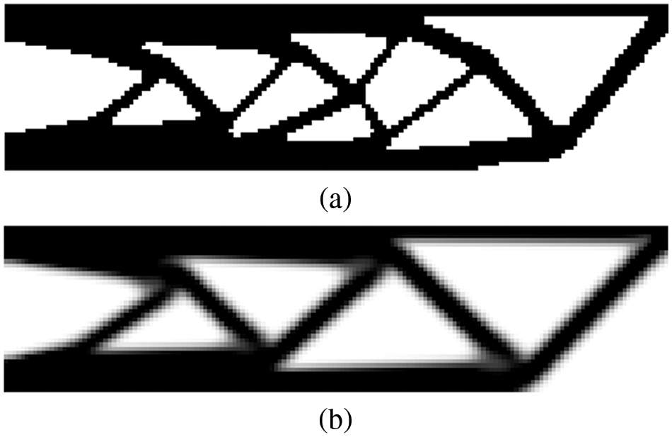
Figure 4: A comparison of BESO and SIMP methods: (a) soft-kill BESO with ER = 2% and p = 3, and (b) SIMP with p = 3

Huang et al. [13] provided a soft-kill BESO Matlab code (BESO2D) and systematically discussed the BESO for various problems, including displacement constraint, natural frequency, nonlinear and energy absorption. More BESO codes for both 2D and 3D problems can be downloaded from website https://www.rmit.edu.au/research/centres-collaborations/centre-for-innovative-structures-and-materials/software. Xia et al. [52] published two Matlab codes (esoL and esoX) based on the hard-kill BESO method, which can be used for benchmark designs and material microstructures, respectively (see Fig. 5). Recently, Lin et al. [53] introduced a BESO method with a dynamic evolution rate for both 2D and 3D problems and presented a 390-line code (DER-BESO) written in ANSYS Parametric Design Language (APDL). Recently, Han et al. [54] proposed an easy-to-implement and comprehended 137-line Matlab code (BESO137) for geometrically nonlinear TO using the BESO method (only 118 lines are necessary, excluding 19 lines for explanation).

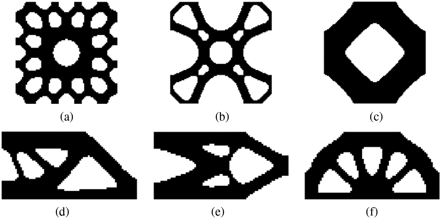
Figure 5: Optimized results of the Matlab codes esoX and esoL. (a) esoX: Material bulk modulus maximization with 60% volume constraint, (b) esoX: Material bulk modulus maximization with 40% volume constraint, (c) esoX: Shear bulk modulus maximization with 60% volume constraint, (d) esoL: Half-MBB beam, (e) esoL: Cantilever, and (f) esoL: Half wheel

4.3 Evolutionary Topology Optimization with Smooth Boundary

ESO/BESO methods always generate black-and-white optimized results, however they suffer from a weak capability of boundary representation due to the finite element mesh. This restriction makes it difficult for these methods to generate smooth and manufacturable CAD models. To solve this problem, Liu et al. [55] proposed a fixed-grid BESO (FG BESO) method that allowed the boundaries of the design to cross finite elements to obtain smoother boundaries; However, the results on the boundaries were inaccurate because the element stiffness was assumed to be proportional to the area fraction of the solid material within the element. Abdi et al. [56] introduced the extended finite element method (XFEM) with evolutionary TO to obtain smooth boundaries of optimized results for 2D problems, where isolines represented their boundaries.

Da et al. [57] introduced the implicit level-set function constructed based on sensitivity analysis to describe the structural topology with smooth boundary representation and suggested an evolutionary topology optimization method based on the BESO method. The corresponding Matlab code (ETO) is given in [57] as the Appendix and can be downloaded from the website https://github.com/Daicong-Da/Evolutionary-topology-optimization. From the results of ETO shown in Fig. 6, it is easy to find that the boundaries are much smoother than those of conventional BESO methods.

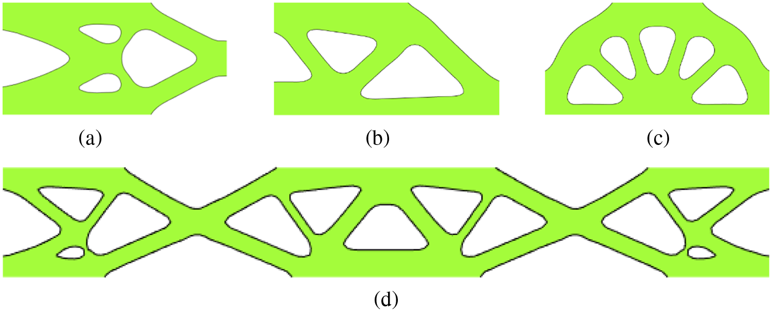
Figure 6: Optimized results of the Matlab code ETO: (a) cantilever, (b) MBB beam, (c) half wheel, and (d) clamped beam

Wang et al. [58] recently presented a multi-resolution TO based on the BESO and XFEM (M-BESO). By introducing enriched nodes to divide a finite element of analysis into sub-triangles, this method can generate high-resolution designs while preserving the topological complexity with less degrees of freedoms (DOFs). In other works, the coarser analysis element is utilized in FEA, whilst the finer sub-triangles are used to describe material properties.

5  The TO Based on the Level Set Method

The TO based on the level set method (LSM) employs a higher dimensional level set function to describe structural geometries implicitly, which can easily trace the boundary of structures during the TO procedure. This section will review the theory and open-source codes of LSM based TO methods.

5.1 Introduction of the TO Based on Level Set Method

The level set-based TO method (see Fig. 7) has received extensive attention, as well as SIMP and ESO/BESO. The LSM was first proposed by Osher et al. in 1988 [59]. This method uses an implicit expression to describe the evolution process of the moving boundary through the zero-level set of a high-dimensional function. Due to the implicit expression, the LSM overcomes the problem of complex boundary collision detection when the topology changes in the previous explicit expression to describe the boundary evolution process.

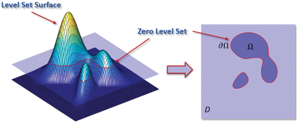
Figure 7: The level set approach employs the zero-contours of high-dimensional implicit functions to describe structural design boundaries [60]

Around 2003, Wang et al. [10] and Allaire et al. [11] first adopted the sensitivity analysis method based on shape derivatives. They applied the LSM to the field of TO, opening up a new research direction [19].

First, a sufficiently large fixed reference domain D is defined that completely contains the solid domain Ω, i.e., Ω ⊆ D. Domain boundary ∂Ω is implicitly embedded through a higher dimensional level set function ϕ(x) such that ∂Ω = {x: x∈D, ϕ(x) = 0}. In addition, the inside-outside functions are defined as follows:

{ϕ(x)>0,∀x∈Ω∖∂Ωϕ(x)=0,∀x∈∂Ωϕ(x)<0,∀x∈D∖∂Ω(10)

Thus, the mathematical model for TO based on LSM can be given by

Minϕ:J(u,ϕ)=∫DF(u)H(ϕ)dΩSubject to:a(u,v,ϕ)=L(v,ϕ),∀v∈UV(ϕ)≤V∗(11)

where the objective function J is minimized for a specific physical or geometric type described by F, U represents the space of kinematically admissible displacement fields, a ( u, v, ϕ), L ( v, ϕ), and V(ϕ) are the strain energy in bilinear form, the load in linear form and the volume of the structure, respectively described by

a(u,v,ϕ)=∫DEijklεij(u)εkl(v)H(ϕ)dΩL(v,ϕ)=∫DpvH(ϕ)dΩ+∫Dτvδ(ϕ)|∇ϕ|dΩV(ϕ)=∫DH(ϕ)dΩ(12)

where Eijkl is the elasticity tensor, eij is the strain tensor, p and τ represent thebody forces and the boundary tractions, respectively, the Heaviside function H and the Dirac function δ are specified as follows:

H(ϕ)={1,ϕ≥00,ϕ≤0,δ(ϕ)=dHdϕ(13)

The introduction of the LSM provides a new class of optimization models for the field of TO, which stimulates the research interest of many scholars all over the world. At present, the TO method based on a level set has been applied to the TO research of many kinds of problems, including stiffness [10], strength [61], stability [62], compliance mechanism [63], heat conduction [64], fluids [65], electromagnetic fields [66], and other problems. The LSM is still a research hotspot in the field of structural TO.

5.2 Open-Source Codes of LSM Based TO

The earliest public code of the level set method should be the 199-line Matlab code (TOPLSM) published by Chen in 2004 [67]. This code provides a complete TO process based on the traditional LSM, including FEA, sensitivity calculation, re-initialization, and result display. It is suitable for readers who are new to level-set-based TO to get started. In this code, the structural boundary evolution is controlled by solving the traditional Hamilton-Jacobi equation of level set evolution, as shown in Eq. (14).

∂ϕ∂t+Vn|∇(ϕ)|=0(14)

where Vn is “speed function” which defines the “speed” of propagation of all level sets of the embedding function ϕ.

Allaire et al. [68] also provided a TO program, developed in FreeFem++ scripting language, again using the traditional level set method. This code uses FreeFem++ as the finite element solver, which has higher computational efficiency and extensibility. This program can solve more complex unstructured mesh problems and provides shape and topology optimization algorithms. Later, Challis proposed [14] the LevelSet129 for level set TO. The code applies a traditional LSM similar to the previous two, but the main difference is that the level set updating scheme shown in Eq. (15).

∂ϕ∂t=−v|∇ϕ|−wg(15)

where w is a positive parameter which determines the influence of the term involving g. Different from Eqs. (14), (15) adds a topological derivative-related term to the H-J equation so that new holes can be automatically generated in 2D optimization problems. In addition, the volume constraints in the procedure are handled by the augmented Lagrangian multiplier method [69], while the fixed Lagrange multiplier method is used in the previous two codes.

In 2015, Otomori et al. [70] released a Matlab code (LevelSet88) for level set topology optimization based on the reaction-diffusion method. In this code, Eq. (16) is used to update the level set function [71].

∂ϕ∂t=−K(F¯′−τ∇2ϕ)(16)

where K > 0 is a coefficient of proportionality, F¯′ is the topological derivative, which is quite different from the previous level set topological optimization methods based on the H-J equation and shape derivatives. In addition, this diffusion term ∇2ϕ can make the boundary smoother as the parameter τ increases and get more concise optimization results. The effect of this item corresponds to the perimeter constraint added to Allaire's code. However, because the derivation and calculation process of topological derivatives are complicated, which is not easy for beginners to study, there will also be difficult to other problems such as dynamics, heat transfer, and compliant mechanisms optimization problems.

Laurain [72] provided a level-set TO code based on the FEniCS (LevelSetFE) (https://fenicsproject.org/). This code is developed based on Python. Since both Python and FEniCS are powerful free resources, this program is helpful for beginners to study. Moreover, FEniCS has powerful finite element analysis and parallel calculation functions, so that program can achieve powerful TO functions after expansion. This paper adopts the traditional level set algorithm and adopts the calculation and derivation based on shape derivatives. A deep understanding of the method in this paper requires familiarity with the derivation and symbolic system of shape derivatives [11]. This may be difficult for beginners in TO, starting from the SIMP method. Fortunately, the author provides optimization codes for mean compliance and compliance mechanism (http://antoinelaurain.com/recherche_eng.htm), which is very helpful to readers familiar with Python. Moreover, Kambampati et al. [73] published an Open source software for Level Set TO (OpenLSTO) written in C++, which contains two modules: FEA module that can be able to perform finite element analysis, and LSM module that can be able to perform design optimization using the LSM.

Wei et al. [69] also published an 88-line parameterized level set topology optimization code (TOPRBF) in 2018. This article improves the parameterized level set method of Wang and Wang in 2006 [74]. The update scheme of the level set function is replaced from a PDE update format with an ordinary differential equation (ODE) update format. In this equation, |∇(ϕ)| in Eq. (14) is replaced by δ(ϕ), and the improved iterative update scheme is as follows:

∂ϕ∂t+Vn⋅δ(ϕ)=0(17)

This iterative update scheme was first applied by Wang et al. [75]. In [60], the concept of the level set band is introduced by changing the parameters of the δ function in Eq. (14), which can combine the advantages of the variable density method to improve the optimization effect further. Due to the ODE update method, the automatic generation of internal holes can be realized, which is essentially similar to Eq. (16).

Yaghmaei et al. [76] published a 62-line topological derivative-based level set TO code (LevelSet-62) using a method similar to Otomori et al. [70] with an iterative update format of Eq. (16) but without introducing a diffusion term. Thus, using the finite element method to solve the PDE of Eq. (17) can be avoided to save computation cost. Meanwhile, Andersen et al. [77] released a MATLAB code (topcut) for implementing level set topology and shape optimization by density methods using cut elements with length scale control.

Liu et al. [78] combined the LSM with the variable density-based method by using the sensitivity derivation of the SIMP method and the boundary representation with the LSM. The combination of different methods taking advantages of their respective advantages has been a new trend in the field of TO in recent years. In their work, the penalty factor of SIMP is retained as a parameter. The evolution of the structural boundary adopts the LSM of the ODE format, which not only simplifies the calculation but also makes the boundary smoother. The article provides 2-D (LevelSet58, LevelSet62 and LevelSet63) and 3-D (LevelSet3D105, LevelSet3D108 and LevelSet3D80) MATLAB codes for multiple problems, including compliance minimization, eigenvalue maximization and thermal compliance minimization, which are very helpful for beginners in different research directions to study and get started.

Wang et al. [79] published a paper about Matlab codes for Velocity Field LSM. This article provides 80-line 2D (VFLSM) and 100-line 3D (VFLSM_3D) TO codes. Like the previous Chen’s 199-line and Challis's codes, these two programs also use the traditional level set iterative update format, but the difference is that the traditional LSM often uses the steepest descent method as the optimization algorithm, in which the velocity field is taken as the opposite value of the shape derivative. This optimization method is relatively simple and easy to understand, but inefficient, and not good at dealing with multi-constraint problems. Therefore, this article uses MMA to optimize the velocity field by directly calculating the sensitivity of the objective function with respect to the velocity field and then uses the LSM to update the boundary iteratively. This method can easily deal with multi-constraint optimization problems and improve computational efficiency.

Some optimized results by the TOs using LSM are shown in Fig. 8, where we can find that the boundaries of results are smooth. This demonstrates that it is easy to generate smooth results by the TOs based on LSM.

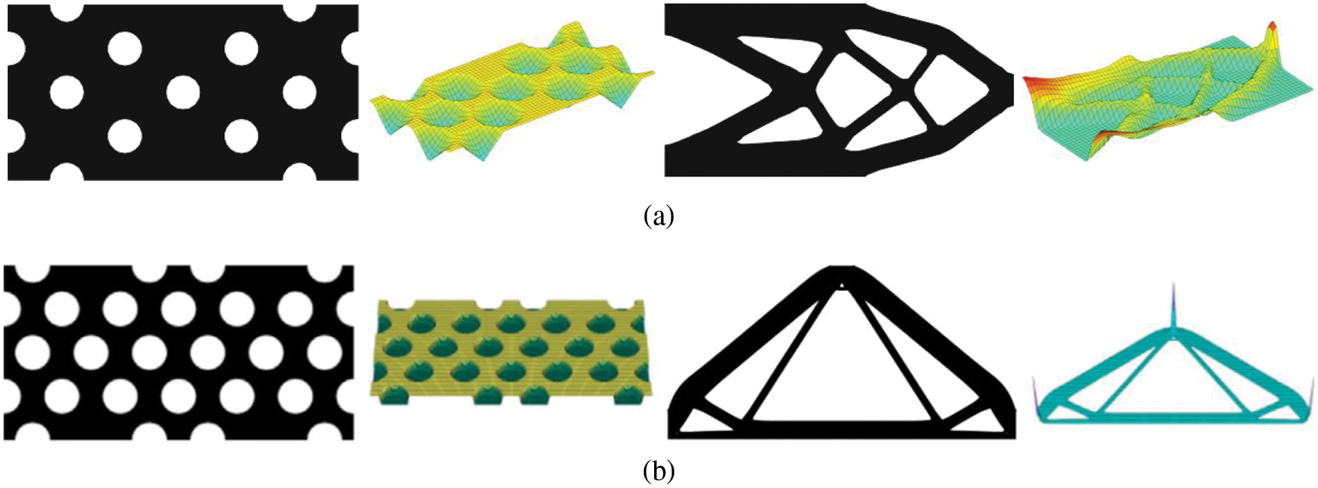
Figure 8: Optimized results of Matlab TO codes using LSM: (a) TOPRBF [69], and (b) LevelSet58 [78]

6  Explicit Geometric TO

Many researchers have recently aimed to make the TO more explicit and flexible. Therefore, a new set of TO methods combining discrete movable components in a weak background mesh has been developed and studied in the recent decade. This section will introduce some explicit TO methods and their open-source codes.

6.1 SSM-Based TO

The stiffness spreading method (SSM) is the first explicit TO method by combining discrete bar elements proposed by Wei et al. in 2010 [80]. In SSM, the stiffness matrices of discrete bars or components are transformed to a background mesh without involving additional DOFs. The sensitivity of the parameters, like the locations of nodes and cross sections of bars, can be derived to optimize the layout of the whole structure. A background structure filled with weak material is used to prevent singularity in finite element analysis; thus, bars or components can move freely in the design domain without necessarily being connected during the optimization process. The stiffness spreading method provides a new concept for TO. Fig. 9 shows some optimization examples based on the stiffness spreading method, such as for a truss optimization problem [80,81] (the corresponding code SSM is available at https://github.com/PengWeiScut/SSM), a modified stiffness spreading method using bars to replace the continuum as the background structure [82], and an integrated optimization problem for a heat-transfer system [83]. This method can also be applied to spread the stiffness of stiffeners of plates and shells in optimization of the stiffener layout [84,85].

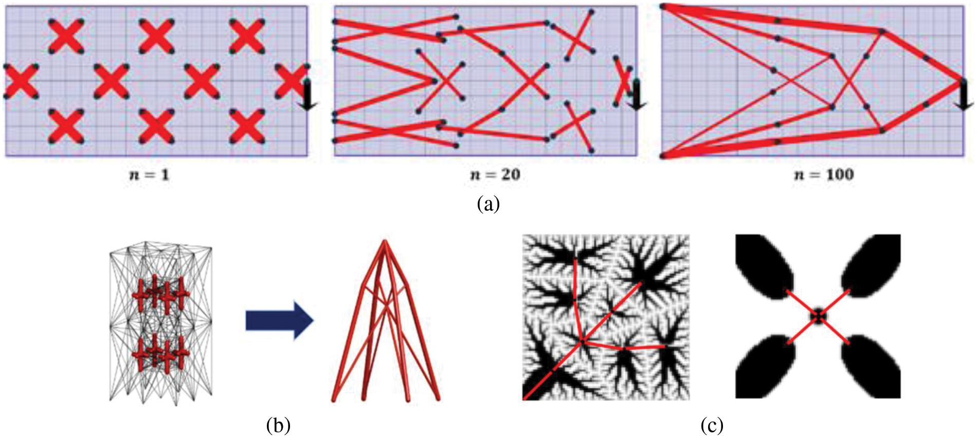
Figure 9: Examples of topology optimization with stiffness spreading method: (a) SSM for truss structures layout optimization [81], (b) Improved stiffness spreading method for truss layout optimization [82], (c) Integrated optimization with stiffness spreading method for heat-transfer system optimization [83]

6.2 MMC-Based TO

To establish a connection between TO and computer-aid-design (CAD) modeling systems, Guo et al. [86] proposed a novel TO method based on the moving morphable component (MMC) framework to explicitly represent the TO geometry. In the MMC framework, different structures are constituted by a series of components, and the structures can be changed by changing the geometry characteristic parameters of these components, such as the shape, length, thickness and layout. Therefore, the design variables are the parameters of the components. This approach can significantly reduce the number of design variables and improve computational efficiency, especially for cases with large design domains. Moreover, since the structural information of the optimized results is explicitly provided, the optimized results can be imported into CAD software for modeling corresponding structures. In the MMC framework, topology description can be achieved in the following way:

{φs(x)>0,∀x∈Ωφs(x)=0,∀x∈∂Ωφs(x)<0,∀x∈D∖(Ω∪∂Ω)(18)

with

φs=max(φ1,…,φi,…,φn)(19)

and

{φi(x)>0,∀x∈Ωiφi(x)=0,∀x∈∂Ωiφi(x)<0,∀x∈D∖(Ωi∪∂Ωi)(20)

where D is the design domain. Ω denotes the solid material region occupied by n solid components. Ωi is the structural region composed of ith component and ∂Ωi is the boundary of Ωi. The topology description function (TDF) of the component can be represented by its geometry information, including the center coordinates, half length, inclined angle, and variable depth.

Zhang et al. [15] improved the MMC-based TO method in 2D problems in the aspects of geometry description functions and the material model. In the work of Zhang et al. [15], the MMC-based TO method was introduced in detail, and an open-source 188-line code (MMC188) of the MMC-based TO for 2D problems was provided. Afterward, Zhang et al. [87,88] applied the MMC-based TO methods to solve multi-material and 3D TO problems. Recently, Du et al. [89] provided a 256-line Matlab code (MMC3D256) for 3D problems and also proposed a 218-line Matlab code (MMC218) for 2D problems. They improved the accuracy of sensitive analysis and removed the DOFs that did not belong to the load transmission path. Furthermore, the MMC method was also applied to isogeometric TO [90], multi-resolution TO [91], thermal-fluid problems [92], metamaterials design [93], etc. Fig. 10 exhibits the optimized results of MMC-based TO.

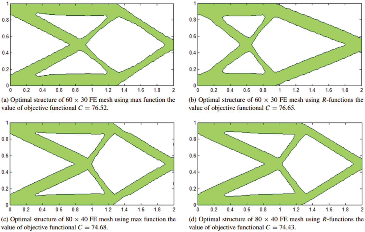
Figure 10: The TO results of the max function and R-functions with different FE meshes [90]

6.3 MMV-Based TO

In order to achieve the explicit and smooth curve of the boundary of optimal structural topology, Zhang et al. [94] proposed the basic theories of the moving morphable void (MMV) framework were first introduced in this work. The TO based on the MMV method shares a similar theory background with the MMC-based TO and is viewed as the formulation of the MMC-based method. But unlike the MMC method, the MMV method introduces some deformable voids. The deformation, intersection, and emergence of the voids generate the void domain of the design domain (see Fig. 11). The parameters of the geometry description of those voids are the design variables in the MMV framework. The MMV-based method can reduce the number of design variables, which improves the optimization efficiency to a large extent.

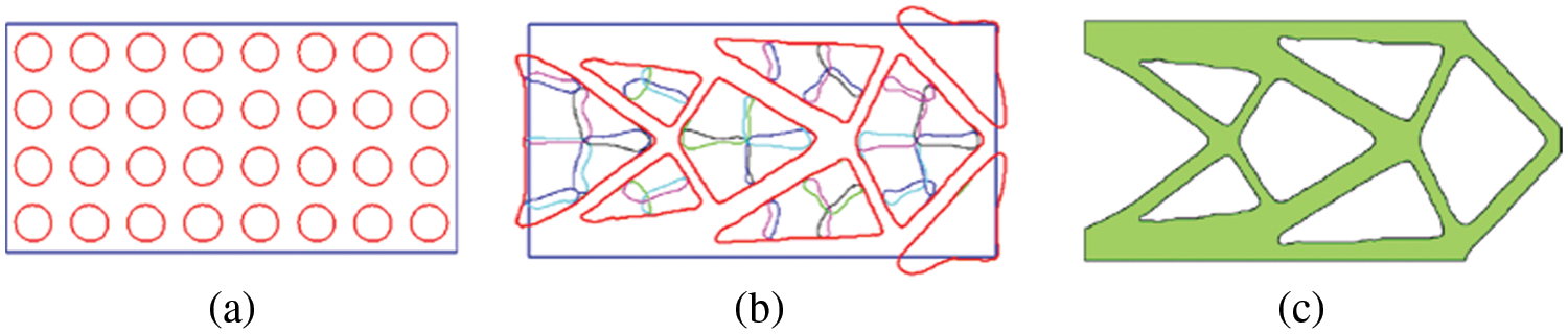
Figure 11: MMV-based topology optimization of a short beam structure: (a) initial design, (b) optimized structure (B-spline plot), and (c) optimized structure (contour plot) [94]

The MMV-based TO has also been applied to many problems. Zhang et al. [95] used it to solve 2D stress-constraint problems. Explicit control problems of structural complexity are considered by Zhang et al. [96] and Zhang et al. [97]. Du et al. [98] proposed an MMV-based TO using the B-spline curves and Kreisselmeier–Steinhauser function to improve the smoothness of the structural boundary. The MMV method was also applied to iso-geometry TO. (A MATLAB code (IGAMMV) of the IGA-MMV TO is available at https://github.com/CMU-CBML/HXTO/tree/main/MMA_MMV). Thereafter, Du et al. [99] innovatively applied the modified MMV method to the design of topological materials to systematically obtain optimized valley Hall insulators.

6.4 MMB-Based TO

Another extension of the MMC method is the moving morphable bar (MMB) method, which employs a series of bars to construct the topology of structures. The MMB-based method can achieve versatile thickness control, including minimum and maximum thickness control, uniform thickness control, multiple thickness control, etc. [100]. The geometric parameters of the moving bars are considered as the design variables in the MMB framework (see Fig. 12). Hoang et al. [100] proposed the MMB-based framework and alleviated the numerical difficulties of solving the hinge designs in a compliant mechanism. Wang et al. [101] then improved the MMB method and introduced an optimization model for integrated layout design of multi-component systems composed of multi-phase materials. Zhao et al. [102] provided a basic 3D Matlab code (MMB3D) for solid MMB-based TO, which has been illustrated in detail in this work, and also expanded the code to be suitable for hollow MMBs. Wang et al. [103] proposed a new TO method based on the MMB framework for the problem of embedding variable-size movable holes into the design domain and realizing multi-material optimization.

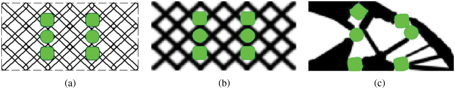
Figure 12: MMB-based topology optimization of a short beam structure: (a) initial design with 48 bars, (b) optimized moving bars, and (c) optimized structure [101]

6.5 Geometric Projection TO

The geometry projection (GP) method is another explicit TO method which describes the geometry of the moving bars by the element density. The density was calculated by the area/volume fraction of the solid inside a circular sampling window. This kind of TO method has the advantage of fabricating the design with off-shelf stock material. Norato et al. [104] proposed and applied the GP framework to shape optimization. Then, Norato et al. [105] employed the previous GP algorithm for continuum-based TO problems, as shown in Fig. 13. Kazemi et al. [106] proposed a new GP approach for the simultaneous TO and material selection of structures, allowed each of the design domain components to be made of different materials. The GP method was also extended to plate structures [107], 3D open lattices composed of single or multiphase materials [108], and stress-based TO problems [109]. Smith et al. [110] introduced the GP method in detail and demonstrated the implementation of geometry mapping using vectorized operations. In the work of Smith et al. [110], a Matlab code (GPTO) was also proposed, and an overview introduction of this code was provided (the completed code is available through GitHub at https://github.com/jnorato/GPTO). Furthermore, Coniglio et al. [111] proposed a Generalized GP method, which unified the GP method, MMC method, and Moving Node method and presented a corresponding MATLAB code (GGP) at https://github.com/topggp/GGP-Matlab.

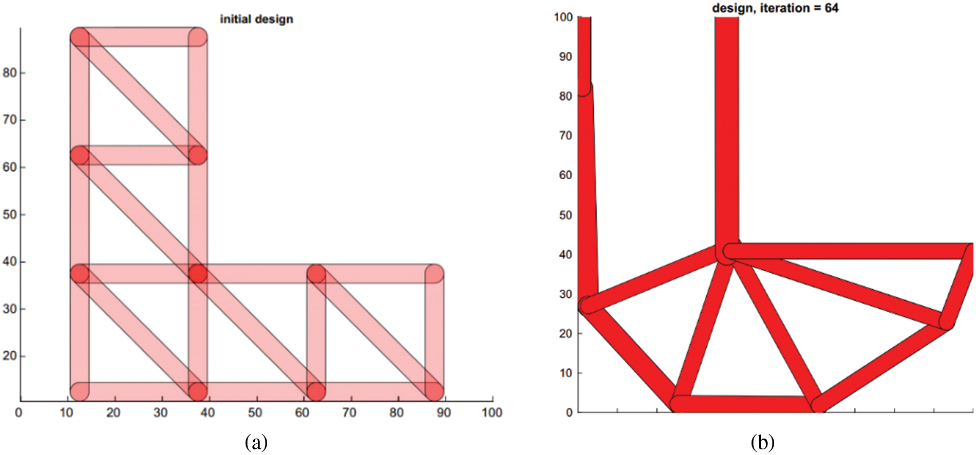
Figure 13: GP-based topology optimization of L-bracket: (a) initial design and (b) optimized design bar layout [110]

7  Multiscale TO

In multiscale TOs, both layouts of macro- and micro-structures are taken into consideration. Therefore, a multiscale TO can be regarded as a mono-scale TO and microstructural TO. In this section, we will briefly review of microstructural TOs before introducing the multiscale TO methods. Some open-source codes are introduced here for both the design of microstructures and the multi-scale topology optimization.

7.1 TO of Microstructures

The theory of homogenization can be used to calculate effective properties of periodic structures and the design of a microstructure with desired properties is known as inverse homogenization. Andreassen et al. [38] provided an efficient way to determine the effective macroscopic properties of the microstructures based on the numerical homogenization theory. In their work, the numerical homogenization method was extended to homogenization of conductivity, thermal expansion, and fluid permeability. The Matlab code of the proposed method can be downloaded from the Appendix of the paper.

TO was first extended to the material design by Sigmund [112] via an inverse homogenization approach using numerical homogenization. Soon after, the inverse homogenization method became the major tool in the design of microstructures. The mathematical formulation of the optimization problem is given in [39] as follows:

Minimizeρ:c=f(EijklH(ρ))Subject to :KUA(kl)=F(kl),k,l=1,…,d:∑e=1Nνeρe/|Y|≤ϑ:0≤ρe≤1,e=1,…,N(21)

Xia et al. [39] proposed a TO method for a material design using the energy-based homogenization method, where the average stress and strain theorems are adopted to predict material effective properties. In this paper, the energy-based homogenization method was briefly reviewed and the Matlab implementation was explained. A 119-line TO code (topX) based on the energy-based homogenization method was presented, which can be found in the Appendix of the above paper. The code allows to be extended to maximize or minimize objective functions constituted by homogenized stiffness tensors such as bulk modulus, shear modulus and Poisson’s ratio. Dong et al. [113] provided a short, self-contained MATLAB homogenization code (homo3D) for 3D cellular materials, which can help readers know more about the homogenization method.

7.2 Multiscale TO Method

Wu et al. [114] reviewed the variety of multi-scale methods and categorized the various multi-scale approaches by (1) the restrictions that applied to the density distribution and (2) the restrictions that applied to the admissible set of properties Ead that can be achieved by parameterized microstructures. The following statement describes the multiscale optimization structure problem:

maxρminuk∈U{maxEH(ρ)∈Ead{ε(uk,ρ)}−∑k=1nloadωkΠextk}(22)

where ρ is the macroscale variable describing the porosity of the varying microstructures, which is subjected to an upper bound on the available material Vmax. EH describes the homogenized elasticity tensor of the microstructures, which has to be in the physically admissible set of elasticity tensors Ead. The inner problem describes the minimization of potential energy Πextk, i.e., the equilibrium constraint that has to hold for each load case k, where the displacement field uk is solved in the space of kinematically admissible displacement fields U. ωk is a weighting factor to scale the energy for each load case. The point-wise optimal strain energy can be written as

ε=12∑k=1nloadωk(∫Ωε(uk):EH(ρ):ε(uk)dΩ)(23)

Gao et al. [115] presented the MATLAB programs for concurrent TO of 2D (ConTop2D) and 3D (ConTop3D) multiscale composite structures. The energy-based numerical homogenization is employed to calculate the effective properties of the microstructures. The TO is executed concurrently at both micro- and macro-scales, with the purpose of simultaneously designing structural layout in two different scales. This method can be extended easily to deal with the optimization problem with different boundary and load conditions. Users can obtain the target macro, and micro-structures after applying the corresponding boundary conditions and load conditions. Different microstructures can be obtained due to the change in the initial design of microstructures.

Four types of MATLAB code are presented in [115], which can be found in the Appendix: (1) the TO codes of cellular composite structures, (2) the codes to compute the 3D isoparametric element stiffness matrix, (3) the energy-based homogenization method codes to predict the macroscopic properties of 2D and 3D material microstructures, and (4) the codes to calculate the sensitivities of the objective function with respect to the design variables at two scales.

Watts et al. [116] provided simple, accurate surrogate models of the homogenized linear elastic response of the isotruss, the octet truss, and the ORC truss using high-fidelity continuum FEA. To show the improvements in compliance relative to a single-scale SIMP design, the method proposed in the paper modified a “standard” single-scale TO code to employ these surrogate models to perform multiscale optimization with a spatially varying relative density unit cell and provided 2D and 3D results, as shown in Fig. 14. To create the surrogate models for the microstructures, the elastic response of the pre-selected microstructures needs to be precomputed, which can be looked up during the macroscale optimization. The pre-computation process might cause additional time consumption but can effectively reduce the computation time for each iteration during the process of optimization. A 3D multiscale TO code (MultiscaleTopOpt) is provided in the Appendix of the paper, which can also be downloaded from the website https://github.com/LLNL/MultiscaleTopOpt. To better understand the multiscale TO method, the readers should understand the homogenization method in order to calculate the equivalent mechanical properties of the pre-selected microstructures.

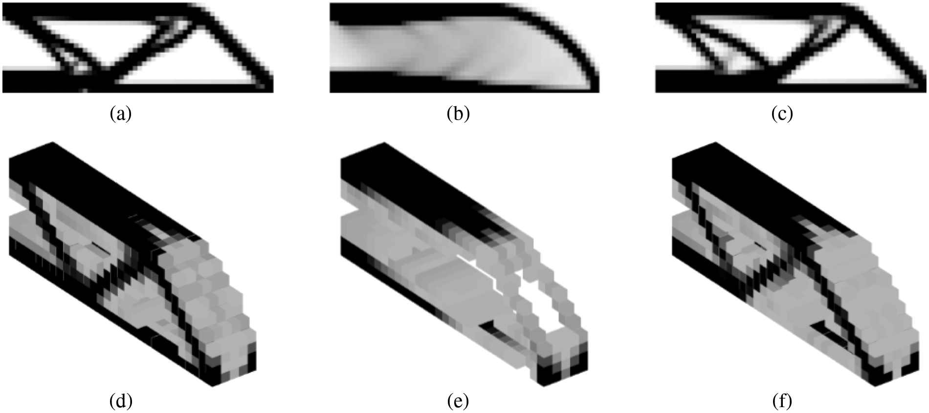
Figure 14: Designs which minimize the compliance of the MBB beam: (a) 2D-SIMP, (b) 2D-Hashin-Shtrikman, (c) 2D-isotruss, (d) 3D-SIMP, (e) 2D-Hashin-Shtrikman, and (f) 3D-isotruss material models

8  Other TOs and Their Applications for Different Problems

Many other TO methods are also presented to solve different types of problems. In this section, we will summarize some of them which provides open-source codes.

8.1 Topology Optimization Using the Independent, Continuous and Mapping Method

Sui et al. [117,118] developed an independent, continuous and mapping (ICM) method for TO problems, where the design variables (called independent topology variables) are independent of elemental physical parameters (e.g., element density). In the ICM method, the polish function and filter function are proposed as the continuous approximation functions of the step function and hurdle function, respectively, which are used to establish a smooth model of TO with continuous variables in the range of [0, 1]. Three kinds of polish functions are given in [118] as follows:

ti=(vivi0)1γ(λ≥1)(24)

ti=1−e(−δvivi0)1−e−δ(δ≥1)(25)

ti=(1+e−α1−e−α)(1−e(−αvivi0)1+e(−αvivi0))(α≥1)(26)

where ti denotes the topology variable, vi is a low-level variable and vi0 is its upper limit. For different TO methods, and vi can be different variables, e.g., vi=ρip for the variable density method like SIMP. Filter functions are the inverse functions of polish functions.

When the 0–1 discrete variable is mapped to the continuous variables, the TO problems can be efficiently solved. After the TO problem is solved, reverse mapping is carried out to map the continuous variables to 0–1 discrete variables. The ICM-based TO has properties of simplicity and rationality, which is suitable for any objective functions. In [119], Sui et al. gave a 120-line TO code (topICM120) based on ICM, and pointed out that the minimization of structural weight with a displacement constraint is more reasonable than the minimum compliance of the continuum structure with sole volume constraint when TO methods are used to solve practical engineering problems.

8.2 Floating Projection TO

Another method using a mapping technique to push the design variables of TO toward 0 or 1 is the floating projection method proposed by Huang [120]. In floating projection topology optimization (FPTO), the floating projection method is used to further modify the filtered design variables ρi¯ as

ρik=tanh⁡(β⋅thk)+tanh⁡[β⋅(ρi¯−thk)]tanh⁡(β⋅thk)+tanh⁡[β⋅(1−thk)](27)

where β>0 controls the steepness of the Heaviside function, and thk is the floating threshold that can be determined by ensuring the summations of design variables are equal before and after the projection, i.e., ∑ρik=∑ρi¯.

The FPTO method can achieve optimized structures with a smooth boundary. A Matlab code (FPTO) is given in [121] by Huang, where the FPTO can be easily implemented within the context of the fixed-mesh finite element analysis and provides an alternative way to form explicit topologies of structures.

8.3 Discrete Variable TO

In addition to continuous variable TO, the discrete variable TO problems have also received attention. Stolpe et al. [122] employed the branch-and-bound method to obtain some globally optimal solutions of discrete variable TO, which became an important benchmark for TO. Liang et al. [123] proposed a relaxation method that can efficiently address the discrete variable structural TO problems with multiple nonlinear constraints or many local linear constraints in a unified and systematic way. Since then, they published a 128-line MATLAB code (DVTOPCRA) [124], which further elaborates discrete variable TO via sequential integer programming and Canonical relaxation algorithm, the results of TO are shown in Fig. 15.

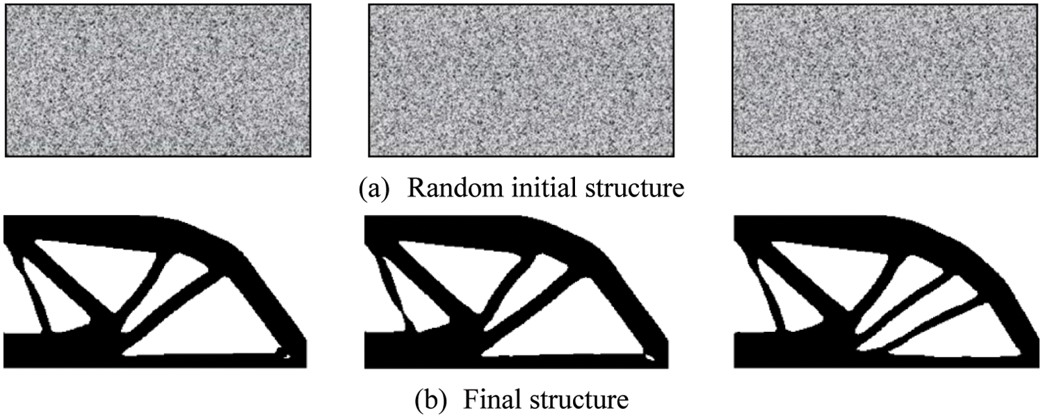
Figure 15: Random initial solutions whose volume fractions are very close to the targeted value 0.5

8.4 Isogeometric TO

Isogeometric topology optimization (ITO) was first proposed by Seo et al. [125], who used the spline surface and trimmed curves to construct a complex design domain without the patch coupling technique. Since then, certain branches of ITO have undergone rapid development in some branches, including density-based ITO [126,127], level set-based ITO [128,129] and ITO using moving morphable components [90,130]. Review paper [131] provided more information regarding ITO.

One of the most important properties of ITO is that the same mathematical representation can be used to describe geometric, analysis and optimization models so that the post-processing is much easier than conventional TOs (Fig. 16 shows a post-processing procedure proposed by Costa et al. [132]). Therefore, the ITO has great potential to directly generate an optimized CAD model without human interaction, which may bring a bran-new design mode for product design in engineering.

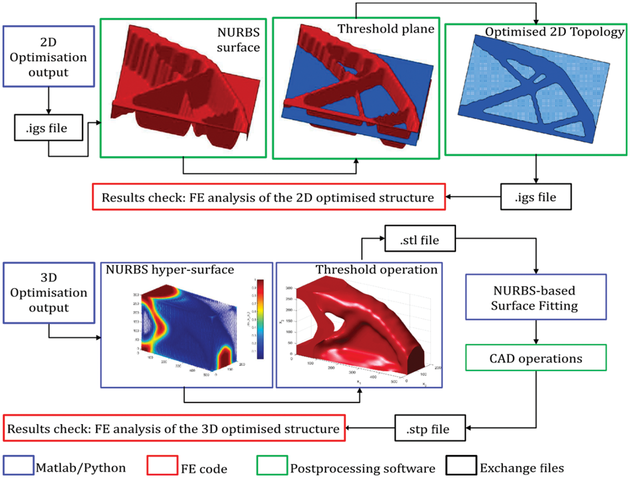
Figure 16: The post-processing procedure proposed by Costa et al. [132]

Gao et al. [133] detailed the ITO technique and gave an open-source Matlab code IgaTop, which inherited the original 88-line SIMP code. The primary content includes the NURBS-based geometrical model, the preparation for IGA, the definition of boundary conditions, the initialization of the DDF at control points and Gauss quadrature points, the definition of the smoothing process, the IGA to solve structural responses, the calculation of the objective function and sensitivity analysis, the update of the design variables and the density distribution function, and the presentation of the optimized designs.

8.5 Non-Gradient-Based TO

Non-gradient topology optimization (NGTO) methods do not require gradients and are easy to implement, which also attract considerable research attention [134]. Biyikli et al. [135] proposed a proportional topology optimization (PTO) by assigning the design variables to elements proportionally to the value of stress in the stress problem and compliance in the compliance problem as follows:

ρiopt=RM∑jNσjqvjσiq(28)

ρiopt=RM∑jNCjqvjCiq(29)

where RM is the remaining material, N is the number of elements, ρioptis the optimized elemental density, σi is the elemental stress, Ci is the elemental compliance value, vj is the elemental volume, and q is the proportion exponent.

PTO can efficiently solve the stress and compliance TO problems, and the open-source MATLAB codes PTOc and PTOs can be downloaded from the website www.ptomethod.org. Wang et al. [136] extended the PTO to solve compliance problems with multiple constraints to design a high-performance hip implant with the porous architecture of optimized graded density.

Najafabadi et al. [137] presented an NGTO method using an adaptive neighborhood simulated annealing (SA), which adaptively adjusted new design variables based on the history of the current solutions and used the crystallization heuristic to smartly control the convergence of the TO problem. The new design variables x are updated by

xnew=xold+1Ci∑1Cirandom(−1/2,1/2)⋅Δri⋅ei(30)

where Δri is the fixed step size of the ith variable, ei is the direction of the ith variable, and Ci denotes the crystallization factor.

The NGTO using an adaptive neighborhood SA has been applied to classic problems of compliance minimization and heat transfer minimization, and the results demonstrate that the method can be used to solve different problems without sensitivity information. The corresponding Matlab code topASA is available on the website https://github.com/Hossein-Rostami/Topology-Optimization-with-adaptive-Simulated-Annealing.

Although the efficiency of NGTO methods is lower as compared to gradient TO methods, they can deal with TO problems without gradients and is easy to implement for complex problems. Therefore, NGTO methods provide us an alternative choice to solve structural TO problems, especially for the unsolvable problems with conventional gradient TO methods.

8.6 Machine Learning TO

Due to the rapid development of machine learning (ML) techniques, ML techniques have also been utilized to reduce computational costs and accelerate the processes of TOs [138,139]. Since the efficiency of ML depends on the number of design variables, ML is especially suitable for the geometry-based TO methods (e.g., MMC and MMB methods) where the number of design variables are much smaller than conventional wise-pixel TO methods, and some successful applications can be found in [140,141]. Huang et al. [142] proposed a problem-independent machine learning technique to reduce the computational time associated with finite element analysis in TO problems. Different from the above methods, Chi et al. [143] proposed a new universal ML-based TO to accelerate the design process of large-scale problems, which collected the training samples simultaneously as the TO proceeds.

Deng et al. [144] proposed a self-directed online learning optimization (SOLO) which integrates deep neural network (DNN) with finite element calculations, and the MATLAB and Python code (SOLO) are available from the website https://github.com/deng-cy/deep_learning_topology_opt. The method was tested by the problems of compliance minimization, fluid-structure optimization, heat transfer enhancement and truss optimization (see Fig. 17), and the results demonstrated that the proposed method can reduce computational time by 2–5 orders when compared to heuristic methods.

Figure 17: Numerical example results of the SOLO: (a) compliance minimization, (b) fluid-structure optimization, (c) heat transfer enhancement and (d) truss optimization [144]

Chandrasekhar et al. [145] proposed a topology optimization using neural networks (TOuNN). In this method, the activation functions of neural networks (NN) are used to represent the SIMP density field so that the density representation can be independent of the finite element mesh, and the sensitivity of loss functions can be analytically computed based on the backpropagation of NN. The proposed method was validated by several numerical examples of both 2D and 3D problems, and a series of properties were investigated, such as computational cost, NN size dependency, and the effect of the mesh size. The corresponding Python code (TOuNN) of this paper is available at www.ersl.wisc.edu/software/TOuNN.zip.

9  Conclusions

In this paper, we summarize the open-source codes of TO methods, including SIMP, ESO/BESO, level-set TO, explicit geometric TO, multiscale TO, ITO, marching learning TO, etc., with the purpose of helping beginners study and understand TO methods. Although we try our best to make this paper more understandable and only introduce the representative open-source codes, more than 60 codes are still presented in this paper. To help beginners learn these TO open-source codes more easily, we divide the codes into five levels, from easy to difficult, according to our experience (see Fig. 18).

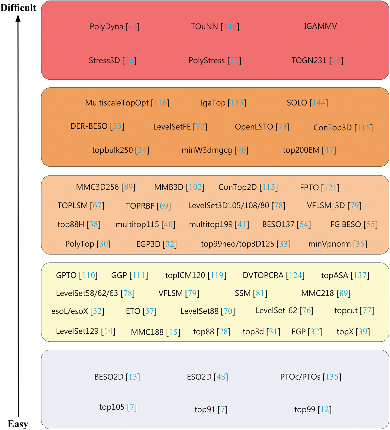
Figure 18: Difficulty classification of the open-source codes mentioned in this paper

Based on Fig. 18, beginners can quickly choose suitable open-source codes to start their research on TO and make their study plan according to their needs and interests. Due to the limited knowledge of the authors, it is impossible to summarize all the open-source codes of TO methods and propose a perfect classification. In the future, the topics of TO may focus on geometric control, additive manufacturing, metamaterials, artificial intelligence, and data-driven. And more relevant open-source codes of TO will be shared to promote the development of TO research, and the sorting and classification of the open-source codes will be further improved.

Funding Statement: This research was supported by the National Key R&D Program of China [Grant Number 2020YFB1708300] and the National Natural Science Foundation of China [Grant Number 52075184].

Conflicts of Interest: The authors declare that they have no conflicts of interest to report regarding the present study.

References

1. Michell, A. G. M. (1904). LVIII. The limits of economy of material in frame-structures. The London, Edinburgh, and Dublin Philosophical Magazine and Journal of Science, 8(47), 589–597. https://doi.org/10.1080/14786440409463229 [Google Scholar] [CrossRef]

2. Prager, W., Rozvany, G. I. N. (1977). Optimization of structural geometry. In: Bednarek, A. R., Cesari, L. (Eds.Dynamical systems, pp. 265–293. New York, USA: Academic Press. [Google Scholar]

3. Rozvany, G. (1972). Optimal load transmission by flexure. Computer Methods in Applied Mechanics and Engineering, 1(3), 253–263. https://doi.org/10.1016/0045-7825(72)90007-2 [Google Scholar] [CrossRef]

4. Cheng, K. T., Olhoff, N. (1981). An investigation concerning optimal design of solid elastic plates. International Journal of Solids and Structures, 17(3), 305–323. https://doi.org/10.1016/0020-7683(81)90065-2 [Google Scholar] [CrossRef]

5. Bendsøe, M. P., Kikuchi, N. (1988). Generating optimal topologies in structural design using a homogenization method. Computer Methods in Applied Mechanics and Engineering, 71(2), 197–224. https://doi.org/10.1016/0045-7825(88)90086-2 [Google Scholar] [CrossRef]

6. Bendsøe, M. P. (1989). Optimal shape design as a material distribution problem. Structural Optimization, 1(4), 193–202. [Google Scholar]

7. Bendsøe, M. P., Sigmund, O. (2003). Topology optimization: Theory, methods and applications. Berlin, Germany: Springer. [Google Scholar]

8. Xie, Y. M., Steven, G. P. (1993). A simple evolutionary procedure for structural optimization. Computers & Structures, 49(5), 885–896. https://doi.org/10.1016/0045-7949(93)90035-C [Google Scholar] [CrossRef]

9. Querin, O., Steven, G., Xie, Y. (1998). Evolutionary structural optimisation (ESO) using a bidirectional algorithm. Engineering Computations, 15(8), 1031–1048. https://doi.org/10.1108/02644409810244129 [Google Scholar] [CrossRef]

10. Wang, M. Y., Wang, X., Guo, D. (2003). A level set method for structural topology optimization. Computer Methods in Applied Mechanics and Engineering, 192(1), 227–246. https://doi.org/10.1016/S0045-7825(02)00559-5 [Google Scholar] [CrossRef]

11. Allaire, G., Jouve, F., Toader, A. M. (2004). Structural optimization using sensitivity analysis and a level-set method. Journal of Computational Physics, 194(1), 363–393. https://doi.org/10.1016/j.jcp.2003.09.032 [Google Scholar] [CrossRef]

12. Sigmund, O. (2001). A 99 line topology optimization code written in Matlab. Structural and Multidisciplinary Optimization, 21(2), 120–127. https://doi.org/10.1007/s001580050176 [Google Scholar] [CrossRef]

13. Huang, X., Xie, M. (2010). Evolutionary topology optimization of continuum structures: Methods and applications. Chichester, England: John Wiley & Sons. [Google Scholar]

14. Challis, V. J. (2010). A discrete level-set topology optimization code written in Matlab. Structural and Multidisciplinary Optimization, 41(3), 453–464. https://doi.org/10.1007/s00158-009-0430-0 [Google Scholar] [CrossRef]

15. Zhang, W., Yuan, J., Zhang, J., Guo, X. (2016). A new topology optimization approach based on moving morphable components (MMC) and the ersatz material model. Structural and Multidisciplinary Optimization, 53(6), 1243–1260. https://doi.org/10.1007/s00158-015-1372-3 [Google Scholar] [CrossRef]

16. Rozvany, G. I. (2009). A critical review of established methods of structural topology optimization. Structural and Multidisciplinary Optimization, 37(3), 217–237. https://doi.org/10.1007/s00158-007-0217-0 [Google Scholar] [CrossRef]

17. Sigmund, O., Maute, K. (2013). Topology optimization approaches. Structural and Multidisciplinary Optimization, 48(6), 1031–1055. https://doi.org/10.1007/s00158-013-0978-6 [Google Scholar] [CrossRef]

18. Deaton, J. D., Grandhi, R. V. (2014). A survey of structural and multidisciplinary continuum topology optimization: Post 2000. Structural and Multidisciplinary Optimization, 49(1), 1–38. https://doi.org/10.1007/s00158-013-0956-z [Google Scholar] [CrossRef]

19. Dijk, N. P., Maute, K., Langelaar, M., Keulen, F. (2013). Level-set methods for structural topology optimization: A review. Structural and Multidisciplinary Optimization, 48(3), 437–472. https://doi.org/10.1007/s00158-013-0912-y [Google Scholar] [CrossRef]

20. Huang, X., Xie, Y. M. (2010). A further review of ESO type methods for topology optimization. Structural and Multidisciplinary Optimization, 41(5), 671–683. https://doi.org/10.1007/s00158-010-0487-9 [Google Scholar] [CrossRef]

21. Mukherjee, S., Lu, D., Raghavan, B., Breitkopf, P., Dutta, S. et al. (2021). Accelerating large-scale topology optimization: State-of-the-art and challenges. Archives of Computational Methods in Engineering, 28(7), 4549–4571. https://doi.org/10.1007/s11831-021-09544-3 [Google Scholar] [CrossRef]

22. Wang, C., Zhao, Z., Zhou, M., Sigmmund, O., Zhang, X. S. et al. (2021). A comprehensive review of educational articles on structural and multidisciplinary optimization. Structural and Multidisciplinary Optimization, 64(5), 2827–2880. https://doi.org/10.1007/s00158-021-03050-7 [Google Scholar] [CrossRef]

23. Boggs, P. T., Tolle, J. W. (1995). Sequential quadratic programming. Acta Numerica, 4, 1–51. https://doi.org/10.1017/S0962492900002518 [Google Scholar] [CrossRef]

24. Hassani, B., Hinton, E. (1998). A review of homogenization and topology optimization III—topology optimization using optimality criteria. Computers & Structures, 69(6), 739–756. https://doi.org/10.1016/S0045-7949(98)00133-3 [Google Scholar] [CrossRef]

25. Svanberg, K. (1987). The method of moving asymptotes—A new method for structural optimization. International Journal for Numerical Methods in Engineering, 24(2), 359–373. https://doi.org/10.1002/(ISSN)1097-0207 [Google Scholar] [CrossRef]

26. Adeli, H., Kumar, S. (1995). Distributed genetic algorithm for structural optimization. Journal of Aerospace Engineering, 8(3), 156–163. https://doi.org/10.1061/(ASCE)0893-1321(1995)8:3(156) [Google Scholar] [CrossRef]

27. Mirjalili, S., Mirjalili, S. M., Lewis, A. (2014). Grey wolf optimizer. Advances in Engineering Software, 69(3), 46–61. https://doi.org/10.1016/j.advengsoft.2013.12.007 [Google Scholar] [CrossRef]

28. Andreassen, E., Clausen, A., Schevenels, M., Lazarov, B. S., Sigmmund, O. et al. (2010). Efficient topology optimization in MATLAB using 88 lines of code. Structural and Multidisciplinary Optimization, 43(1), 1–16. https://doi.org/10.1007/s00158-010-0594-7 [Google Scholar] [CrossRef]

29. Zhou, M., Sigmund, O. (2021). Complementary lecture notes for teaching the 99/88-line topology optimization codes. Structural and Multidisciplinary Optimization, 64(5), 3227–3231. https://doi.org/10.1007/s00158-021-03004-z [Google Scholar] [CrossRef]

30. Talischi, C., Paulino, G. H., Pereira, A., Menezes, I. F. M. (2012). PolyTop: A Matlab implementation of a general topology optimization framework using unstructured polygonal finite element meshes. Structural and Multidisciplinary Optimization, 45(3), 329–357. https://doi.org/10.1007/s00158-011-0696-x [Google Scholar] [CrossRef]

31. Liu, K., Tovar, A. (2014). An efficient 3D topology optimization code written in Matlab. Structural and Multidisciplinary Optimization, 50(6), 1175–1196. https://doi.org/10.1007/s00158-014-1107-x [Google Scholar] [CrossRef]

32. Zeng, Z., Ma, F. (2020). An efficient gradient projection method for structural topology optimization. Advances in Engineering Software, 149, 102863. https://doi.org/10.1016/j.advengsoft.2020.102863 [Google Scholar] [CrossRef]

33. Ferrari, F., Sigmund, O. (2020). A new generation 99 line Matlab code for compliance topology optimization and its extension to 3D. Structural and Multidisciplinary Optimization, 62(4), 2211–2228. https://doi.org/10.1007/s00158-020-02629-w [Google Scholar] [CrossRef]

34. Ferrari, F., Sigmund, O., Guest, J. K. (2021). Topology optimization with linearized buckling criteria in 250 lines of Matlab. Structural and Multidisciplinary Optimization, 63(6), 3045–3066. https://doi.org/10.1007/s00158-021-02854-x [Google Scholar] [CrossRef]

35. Amir, O. (2021). Efficient stress-constrained topology optimization using inexact design sensitivities. International Journal for Numerical Methods in Engineering, 122(13), 3241–3272. https://doi.org/10.1002/nme.6662 [Google Scholar] [CrossRef]

36. Deng, H., Vulimiri, P. S., To, A. C. (2021). An efficient 146-line 3D sensitivity analysis code of stress-based topology optimization written in MATLAB. Optimization and Engineering, 23, 1733–1757. https://doi.org/10.1007/s11081-021-09675-3 [Google Scholar] [CrossRef]

37. Giraldo-Londoño, O., Paulino, G. H. (2021). PolyStress: A Matlab implementation for local stress-constrained topology optimization using the augmented Lagrangian method. Structural and Multidisciplinary Optimization, 63(4), 2065–2097. https://doi.org/10.1007/s00158-020-02760-8 [Google Scholar] [CrossRef]

38. Andreassen, E., Andreasen, C. S. (2014). How to determine composite material properties using numerical homogenization. Computational Materials Science, 83, 488–495. https://doi.org/10.1016/j.commatsci.2013.09.006 [Google Scholar] [CrossRef]

39. Xia, L., Breitkopf, P. (2015). Design of materials using topology optimization and energy-based homogenization approach in Matlab. Structural and Multidisciplinary Optimization, 52(6), 1229–1241. https://doi.org/10.1007/s00158-015-1294-0 [Google Scholar] [CrossRef]

40. Tavakoli, R., Mohseni, S. M. (2013). Alternating active-phase algorithm for multimaterial topology optimization problems: A 115-line MATLAB implementation. Structural and Multidisciplinary Optimization, 49(4), 621–642. https://doi.org/10.1007/s00158-013-0999-1 [Google Scholar] [CrossRef]

41. Zuo, W., Saitou, K. (2016). Multi-material topology optimization using ordered SIMP interpolation. Structural and Multidisciplinary Optimization, 55(2), 477–491. https://doi.org/10.1007/s00158-016-1513-3 [Google Scholar] [CrossRef]

42. Zhang, X. S., Paulino, G. H., Ramos, A. S. (2018). Multimaterial topology optimization with multiple volume constraints: Combining the ZPR update with a ground-structure algorithm to select a single material per overlapping set. International Journal for Numerical Methods in Engineering, 114(10), 1053–1073. https://doi.org/10.1002/nme.5736 [Google Scholar] [CrossRef]

43. Chen, Q., Zhang, X., Zhu, B. (2018). A 213-line topology optimization code for geometrically nonlinear structures. Structural and Multidisciplinary Optimization, 59(5), 1863–1879. https://doi.org/10.1007/s00158-018-2138-5 [Google Scholar] [CrossRef]

44. Giraldo-Londono, O., Paulino, G. H. (2021). PolyDyna: A Matlab implementation for topology optimization of structures subjected to dynamic loads. Structural and Multidisciplinary Optimization, 64(2), 957–990. https://doi.org/10.1007/s00158-021-02859-6 [Google Scholar] [CrossRef]

45. Amir, O., Aage, N., Lazarov, B. S. (2014). On multigrid-CG for efficient topology optimization. Structural and Multidisciplinary Optimization, 49(5), 815–829. https://doi.org/10.1007/s00158-013-1015-5 [Google Scholar] [CrossRef]

46. Amir, O. (2015). Revisiting approximate reanalysis in topology optimization: On the advantages of recycled preconditioning in a minimum weight procedure. Structural and Multidisciplinary Optimization, 51(1), 41–57. https://doi.org/10.1007/s00158-014-1098-7 [Google Scholar] [CrossRef]

47. Christiansen, R. E., Sigmund, O. (2021). Compact 200 line MATLAB code for inverse design in photonics by topology optimization: Tutorial. Journal of the Optical Society of America B–Optical Physics, 38(2), 510–520. https://doi.org/10.1364/JOSAB.405955 [Google Scholar] [CrossRef]

48. Xie, Y., Steven, G. (1997). Evolutionary structural optimization. London: Springer. [Google Scholar]

49. Querin, O., Young, V., Steven, G., Xie, Y. M. (2000). Computational efficiency and validation of bi-directional evolutionary structural optimisation. Computer Methods in Applied Mechanics and Engineering, 189(2), 559–573. https://doi.org/10.1016/S0045-7825(99)00309-6 [Google Scholar] [CrossRef]

50. Rozvany, G. I., Querin, O. M. (2002). Combining ESO with rigorous optimality criteria. International Journal of Vehicle Design, 28(4), 294–299. https://doi.org/10.1504/IJVD.2002.001991 [Google Scholar] [CrossRef]

51. Huang, X., Xie, Y. M. (2009). Bi-directional evolutionary topology optimization of continuum structures with one or multiple materials. Computational Mechanics, 43(3), 393–401. https://doi.org/10.1007/s00466-008-0312-0 [Google Scholar] [CrossRef]

52. Xia, L., Xia, Q., Huang, X., Xie, Y. M. (2018). Bi-directional evolutionary structural optimization on advanced structures and materials: A comprehensive review. Archives of Computational Methods in Engineering, 25(2), 437–478. https://doi.org/10.1007/s11831-016-9203-2 [Google Scholar] [CrossRef]

53. Lin, H., Xu, A., Misra, A., Zhao, R. (2020). An ANSYS APDL code for topology optimization of structures with multi-constraints using the BESO method with dynamic evolution rate (DER-BESO). Structural and Multidisciplinary Optimization, 62(4), 2229–2254. https://doi.org/10.1007/s00158-020-02588-2 [Google Scholar] [CrossRef]

54. Han, Y., Xu, B., Liu, Y. (2021). An efficient 137-line MATLAB code for geometrically nonlinear topology optimization using bi-directional evolutionary structural optimization method. Structural and Multidisciplinary Optimization, 63(5), 2571–2588. https://doi.org/10.1007/s00158-020-02816-9 [Google Scholar] [CrossRef]

55. Liu, Y., Jin, F., Li, Q., Zhou, S. (2008). A fixed-grid bidirectional evolutionary structural optimization method and its applications in tunnelling engineering. International Journal for Numerical Methods in Engineering, 73(12), 1788–1810. https://doi.org/10.1002/(ISSN)1097-0207 [Google Scholar] [CrossRef]

56. Abdi, M., Wildman, R., Ashcroft, I. (2014). Evolutionary topology optimization using the extended finite element method and isolines. Engineering Optimization, 46(5), 628–647. https://doi.org/10.1080/0305215X.2013.791815 [Google Scholar] [CrossRef]

57. Da, D., Xia, L., Li, G., Huang, X. (2018). Evolutionary topology optimization of continuum structures with smooth boundary representation. Structural and Multidisciplinary Optimization, 57(6), 2143–2159. https://doi.org/10.1007/s00158-017-1846-6 [Google Scholar] [CrossRef]

58. Wang, H., Liu, J., Wen, G. (2020). An efficient evolutionary structural optimization method for multi-resolution designs. Structural and Multidisciplinary Optimization, 62(2), 787–803. https://doi.org/10.1007/s00158-020-02536-0 [Google Scholar] [CrossRef]

59. Osher, S., Sethian, J. A. (1988). Fronts propagating with curvature-dependent speed: Algorithms based on Hamilton-Jacobi formulations. Journal of Computational Physics, 79(1), 12–49. https://doi.org/10.1016/0021-9991(88)90002-2 [Google Scholar] [CrossRef]

60. Wei, P., Wang, W., Yang, Y., Wang, M. Y. (2020). Level set band method: A combination of density-based and level set methods for the topology optimization of continuums. Frontiers of Mechanical Engineering, 15(3), 390–405. https://doi.org/10.1007/s11465-020-0588-0 [Google Scholar] [CrossRef]

61. Van Miegroet, L., Duysinx, P. (2007). Stress concentration minimization of 2D filets using X-FEM and level set description. Structural and Multidisciplinary Optimization, 33(4), 425–438. https://doi.org/10.1007/s00158-006-0091-1 [Google Scholar] [CrossRef]

62. Ville, L., Silva, L., Coupez, T. (2011). Convected level set method for the numerical simulation of fluid buckling. International Journal for Numerical Methods in Fluids, 66(3), 324–344. https://doi.org/10.1002/fld.2259 [Google Scholar] [CrossRef]

63. Zhu, B., Zhang, X., Liu, M., Chen, Q., Li, H. (2019). Topological and shape optimization of flexure hinges for designing compliant mechanisms using the level set method. Chinese Journal of Mechanical Engineering, 32(1), 13. https://doi.org/10.1186/s10033-019-0332-z [Google Scholar] [CrossRef]

64. Xia, Q., Shi, T., Xia, L. (2018). Topology optimization for heat conduction by combining level set method and BESO method. International Journal of Heat and Mass Transfer, 127(3), 200–209. https://doi.org/10.1016/j.ijheatmasstransfer.2018.08.036 [Google Scholar] [CrossRef]

65. Deng, Y., Zhang, P., Liu, Y., Wu, Y., Liu, Z. (2013). Optimization of unsteady incompressible Navier-Stokes flows using variational level set method. International Journal for Numerical Methods in Fluids, 71(12), 1475–1493. https://doi.org/10.1002/fld.3721 [Google Scholar] [CrossRef]

66. Okamoto, Y., Masuda, H., Kanda, Y., Reona, H., Shinji, W. (2018). Improvement of topology optimization method based on level set function in magnetic field problem. COMPEL-The International Journal for Computation and Mathematics in Electrical and Electronic Engineering, 37(2), 630–644. https://doi.org/10.1108/COMPEL-12-2016-0528 [Google Scholar] [CrossRef]

67. Chen, S. (2004). Network. http://me.eng.stonybrook.edu/~chen/index_files/downloads.htm [Google Scholar]

68. Allaire, G., CPantz, O. (2006). Structural optimization with FreeFem++. Structural and Multidisciplinary Optimization, 32(3), 173–181. https://doi.org/10.1007/s00158-006-0017-y [Google Scholar] [CrossRef]

69. Wei, P., Li, Z., Li, X., Wang, M. Y. (2018). An 88-line MATLAB code for the parameterized level set method based topology optimization using radial basis functions. Structural and Multidisciplinary Optimization, 58(2), 831–849. https://doi.org/10.1007/s00158-018-1904-8 [Google Scholar] [CrossRef]

70. Otomori, M., Yamada, T., Izui, K., Nishiwaki, S. (2014). Matlab code for a level set-based topology optimization method using a reaction diffusion equation. Structural and Multidisciplinary Optimization, 51(5), 1159–1172. https://doi.org/10.1007/s00158-014-1190-z [Google Scholar] [CrossRef]

71. Takezawa, A., Nishiwaki, S., Kitamura, M. (2010). Shape and topology optimization based on the phase field method and sensitivity analysis. Journal of Computational Physics, 229(7), 2697–2718. https://doi.org/10.1016/j.jcp.2009.12.017 [Google Scholar] [CrossRef]

72. Laurain, A. (2018). A level set-based structural optimization code using FEniCS. Structural and Multidisciplinary Optimization, 58(3), 1311–1334. https://doi.org/10.1007/s00158-018-1950-2 [Google Scholar] [CrossRef]

73. Kambampati, S., Du, Z., Chung, H., Kim, H. A., Hedges, L. (2018). OpenLSTO: Open-source software for level set topology optimization. 2018 Multidisciplinary Analysis and Optimization Conference, Atlanta, USA. [Google Scholar]

74. Wang, S., Wang, M. Y. (2006). Radial basis functions and level set method for structural topology optimization. International Journal for Numerical Methods in Engineering, 65(12), 2060–2090. https://doi.org/10.1002/(ISSN)1097-0207 [Google Scholar] [CrossRef]

75. Wang, M. (2005). Topology optimization with level set method incorporating topological derivative. 6th World Congress on Structural and Multidisciplinary Optimization, Rio de Janeiro, Brazil. [Google Scholar]

76. Yaghmaei, M., Ghoddosian, A., Khatibi, M. M. (2020). A filter-based level set topology optimization method using a 62-line MATLAB code. Structural and Multidisciplinary Optimization, 62(2), 1001–1018. https://doi.org/10.1007/s00158-020-02540-4 [Google Scholar] [CrossRef]

77. Andreasen, C. S., Elingaard, M. O., Aage, N. (2020). Level set topology and shape optimization by density methods using cut elements with length scale control. Structural and Multidisciplinary Optimization, 62(2), 685–707. https://doi.org/10.1007/s00158-020-02527-1 [Google Scholar] [CrossRef]

78. Liu, Y., Yang, C., Wei, P., Zhou, P., Du, J. (2021). An ODE-driven level-set density method for topology optimization. Computer Methods in Applied Mechanics and Engineering, 387, 114159. https://doi.org/10.1016/j.cma.2021.114159 [Google Scholar] [CrossRef]

79. Wang, Y., Kang, Z. (2021). MATLAB implementations of velocity field level set method for topology optimization: An 80-line code for 2D and a 100-line code for 3D problems. Structural and Multidisciplinary Optimization, 64(6), 4325–4342. https://doi.org/10.1007/s00158-021-02958-4 [Google Scholar] [CrossRef]

80. Wei, P., Ma, H., Chen, T., Wang, M. Y. (2010). Stiffness spreading method for layout optimization of truss structures. 6th China-Japan-Korea Joint Symposium on Optimization of Structural and Mechanical Systems, Kyoto, Japan. [Google Scholar]

81. Wei, P., Ma, H., Wang, M. Y. (2014). The stiffness spreading method for layout optimization of truss structures. Structural and Multidisciplinary Optimization, 49(4), 667–682. https://doi.org/10.1007/s00158-013-1005-7 [Google Scholar] [CrossRef]

82. Cao, M., Ma, H., Wei, P. (2018). A modified stiffness spreading method for layout optimization of truss structures. Acta Mechanica Sinica, 34(6), 1072–1083. https://doi.org/10.1007/s10409-018-0776-x [Google Scholar] [CrossRef]

83. Li, Y., Wei, P., Ma, H. (2017). Integrated optimization of heat-transfer systems consisting of discrete thermal conductors and solid material. International Journal of Heat and Mass Transfer, 113(1–2), 1059–1069. https://doi.org/10.1016/j.ijheatmasstransfer.2017.06.018 [Google Scholar] [CrossRef]

84. Liu, H., Li, B., Yang, Z., Hong, J. (2017). Topology optimization of stiffened plate/shell structures based on adaptive morphogenesis algorithm. Journal of Manufacturing Systems, 43(22–23), 375–384. https://doi.org/10.1016/j.jmsy.2017.02.002 [Google Scholar] [CrossRef]

85. Li, B., Liu, H., Yang, Z., Zhang, J. (2019). Stiffness design of plate/shell structures by evolutionary topology optimization. Thin-Walled Structures, 141(2), 232–250. https://doi.org/10.1016/j.tws.2019.04.012 [Google Scholar] [CrossRef]

86. Guo, X., Zhang, W., Zhong, W. (2014). Doing topology optimization explicitly and geometrically—A new moving morphable components based framework. Journal of Applied Mechanics, 81(8), 197. https://doi.org/10.1115/1.4027609 [Google Scholar] [CrossRef]

87. Zhang, W., Song, J., Zhou, J., Du, Z., Zhu, Y. et al. (2018). Topology optimization with multiple materials via moving morphable component (MMC) method. International Journal for Numerical Methods in Engineering, 113(11), 1653–1675. https://doi.org/10.1002/nme.5714 [Google Scholar] [CrossRef]

88. Zhang, W., Li, D., Yuan, J., Song, J., Guo, X. (2017). A new three-dimensional topology optimization method based on moving morphable components (MMCs). Computational Mechanics, 59(4), 647–665. https://doi.org/10.1007/s00466-016-1365-0 [Google Scholar] [CrossRef]

89. Du, Z., Cui, T., Liu, C., Zhang, W., Guo, Y. (2022). An efficient and easy-to-extend Matlab code of the moving morphable component (MMC) method for three-dimensional topology optimization. Structural and Multidisciplinary Optimization, 65(5), 1–29. https://doi.org/10.1007/s00158-022-03239-4 [Google Scholar] [CrossRef]

90. Xie, X., Wang, S., Xu, M., Wang, Y. (2018). A new isogeometric topology optimization using moving morphable components based on R-functions and collocation schemes. Computer Methods in Applied Mechanics and Engineering, 339(2), 61–90. https://doi.org/10.1016/j.cma.2018.04.048 [Google Scholar] [CrossRef]

91. Liu, C., Zhu, Y., Sun, Z., Li, D., Du, Z. et al. (2018). An efficient moving morphable component (MMC)-based approach for multi-resolution topology optimization. Structural and Multidisciplinary Optimization, 58(6), 2455–2479. https://doi.org/10.1007/s00158-018-2114-0 [Google Scholar] [CrossRef]

92. Yu, M., Ruan, S., Wang, X., Li, Z., Shen, C. (2019). Topology optimization of thermal-fluid problem using the MMC-based approach. Structural and Multidisciplinary Optimization, 60(1), 151–165. https://doi.org/10.1007/s00158-019-02206-w [Google Scholar] [CrossRef]

93. Luo, J., Du, Z., Guo, Y., Liu, C., Zhang, W. et al. (2021). Multi-class, multi-functional design of photonic topological insulators by rational symmetry-indicators engineering. Nanophotonics, 10(18), 4523–4531. https://doi.org/10.1515/nanoph-2021-0433 [Google Scholar] [CrossRef]

94. Zhang, W., Yang, W., Zhou, J., Li, D., Guo, X. (2017). Structural topology optimization through explicit boundary evolution. Journal of Applied Mechanics, 84(1), 011011. https://doi.org/10.1115/1.4034972 [Google Scholar] [CrossRef]

95. Zhang, W., Li, D., Zhou, J., Du, Z., Guo, B. (2018). A moving morphable void (MMV)-based explicit approach for topology optimization considering stress constraints. Computer Methods in Applied Mechanics and Engineering, 334, 381–413. https://doi.org/10.1016/j.cma.2018.01.050 [Google Scholar] [CrossRef]

96. Zhang, W., Liu, Y., Wei, P., Zhu, Y., Guo, X. (2017). Explicit control of structural complexity in topology optimization. Computer Methods in Applied Mechanics and Engineering, 324, 149–169. https://doi.org/10.1016/j.cma.2017.05.026 [Google Scholar] [CrossRef]

97. Zhang, W., Chen, J., Zhu, X., Zhou, J., Xue, D. et al. (2017). Explicit three dimensional topology optimization via moving morphable void (MMV) approach. Computer Methods in Applied Mechanics and Engineering, 322(1), 590–614. https://doi.org/10.1016/j.cma.2017.05.002 [Google Scholar] [CrossRef]

98. Du, B., Yao, W., Zhao, Y., Chen, X. (2019). A moving morphable voids approach for topology optimization with closed B-splines. Journal of Mechanical Design, 141(8), 197. https://doi.org/10.1115/1.4043369 [Google Scholar] [CrossRef]

99. Du, Z., Chen, H., Huang, G. (2020). Optimal quantum valley Hall insulators by rationally engineering Berry curvature and band structure. Journal of the Mechanics and Physics of Solids, 135(1802), 103784. https://doi.org/10.1016/j.jmps.2019.103784 [Google Scholar] [CrossRef]

100. Hoang, V. N., Jang, G. W. (2017). Topology optimization using moving morphable bars for versatile thickness control. Computer Methods in Applied Mechanics and Engineering, 317, 153–173. https://doi.org/10.1016/j.cma.2016.12.004 [Google Scholar] [CrossRef]

101. Wang, X., Long, K., Hoang, V. N., Ping, H. (2018). An explicit optimization model for integrated layout design of planar multi-component systems using moving morphable bars. Computer Methods in Applied Mechanics and Engineering, 342(2), 46–70. https://doi.org/10.1016/j.cma.2018.07.032 [Google Scholar] [CrossRef]

102. Zhao, Y., Hoang, V. N., Jang, G. W., Zuo, W. (2021). Hollow structural topology optimization to improve manufacturability using three-dimensional moving morphable bars. Advances in Engineering Software, 152, 102955. https://doi.org/10.1016/j.advengsoft.2020.102955 [Google Scholar] [CrossRef]

103. Wang, X., Long, K., Meng, Z., Yu, B., Cheng, C. (2021). Explicit multi-material topology optimization embedded with variable-size movable holes using moving morphable bars. Engineering Optimization, 53(7), 1212–1229. https://doi.org/10.1080/0305215X.2020.1779710 [Google Scholar] [CrossRef]

104. Norato, J., Haber, R., Tortorelli, D., Bendsøe, M. P. (2004). A geometry projection method for shape optimization. International Journal for Numerical Methods in Engineering, 60(14), 2289–2312. https://doi.org/10.1002/(ISSN)1097-0207 [Google Scholar] [CrossRef]

105. Norato, J., Bell, B., Tortorelli, D. A. (2015). A geometry projection method for continuum-based topology optimization with discrete elements. Computer Methods in Applied Mechanics and Engineering, 293(4), 306–327. https://doi.org/10.1016/j.cma.2015.05.005 [Google Scholar] [CrossRef]

106. Kazemi, H., Vaziri, A., Norato, J. A. (2018). Topology optimization of structures made of discrete geometric components with different materials. Journal of Mechanical Design, 140(11), 111401. https://doi.org/10.1115/1.4040624 [Google Scholar] [CrossRef]

107. Zhang, S., Norato, J. A., Gain, A. L., Lyu, N. (2016). A geometry projection method for the topology optimization of plate structures. Structural and Multidisciplinary Optimization, 54(5), 1173–1190. https://doi.org/10.1007/s00158-016-1466-6 [Google Scholar] [CrossRef]

108. Watts, S., Tortorelli, D. A. (2017). A geometric projection method for designing three-dimensional open lattices with inverse homogenization. International Journal for Numerical Methods in Engineering, 112(11), 1564–1588. https://doi.org/10.1002/nme.5569 [Google Scholar] [CrossRef]

109. Zhang, S., Gain, A. L., Norato, J. A. (2017). Stress-based topology optimization with discrete geometric components. Computer Methods in Applied Mechanics and Engineering, 325(4), 1–21. https://doi.org/10.1016/j.cma.2017.06.025 [Google Scholar] [CrossRef]

110. Smith, H., Norato, J. A. (2020). A MATLAB code for topology optimization using the geometry projection method. Structural and Multidisciplinary Optimization, 62(3), 1579–1594. https://doi.org/10.1007/s00158-020-02552-0 [Google Scholar] [CrossRef]

111. Coniglio, S., Morlier, J., Gogu, C., Amargier, R. (2020). Generalized geometry projection: A unified approach for geometric feature based topology optimization. Archives of Computational Methods in Engineering, 27(5), 1573–1610. https://doi.org/10.1007/s11831-019-09362-8 [Google Scholar] [CrossRef]

112. Sigmund, O. (1994). Materials with prescribed constitutive parameters: An inverse homogenization problem. International Journal of Solids and Structures, 31(17), 2313–2329. https://doi.org/10.1016/0020-7683(94)90154-6 [Google Scholar] [CrossRef]

113. Dong, G., Tang, Y., Zhao, Y. F. (2018). A 149 line homogenization code for three-dimensional cellular materials written in matlab. Journal of Engineering Materials and Technology, 141(1), 011005. https://doi.org/10.1115/1.4040555 [Google Scholar] [CrossRef]

114. Wu, J., Sigmund, O., Groen, J. P. (2021). Topology optimization of multi-scale structures: A review. Structural and Multidisciplinary Optimization, 63(3), 1455–1480. https://doi.org/10.1007/s00158-021-02881-8 [Google Scholar] [CrossRef]

115. Gao, J., Luo, Z., Xia, L., Gao, L. (2019). Concurrent topology optimization of multiscale composite structures in Matlab. Structural and Multidisciplinary Optimization, 60(6), 2621–2651. https://doi.org/10.1007/s00158-019-02323-6 [Google Scholar] [CrossRef]

116. Watts, S., Arrighi, W., Kudo, J., Tortorelli, D. A., White, D. A. (2019). Simple, accurate surrogate models of the elastic response of three-dimensional open truss micro-architectures with applications to multiscale topology design. Structural and Multidisciplinary Optimization, 60(5), 1887–1920. https://doi.org/10.1007/s00158-019-02297-5 [Google Scholar] [CrossRef]

117. Sui, Y. K., Yang, D. Q. (1998). A new method for structural topological optimization based on the concept of independent continuous variables and smooth model. Acta Mechanica Sinica, 14(2), 179–185. https://doi.org/10.1007/BF02487752 [Google Scholar] [CrossRef]

118. Sui, Y., Peng, X. (2018). Modeling, solving and application for topology optimization of continuum structures: ICM method based on step function. Beijing, China: Tsinghua University Press. [Google Scholar]

119. Sui, Y., Yi, G. (2013). A discussion about choosing an objective function and constraint conditions in structural topology optimization. 10th World Congress on Structural and Multidisciplinary Optimization, Orlando, USA. [Google Scholar]

120. Huang, X. (2020). Smooth topological design of structures using the floating projection. Engineering Structures, 208(3), 110330. https://doi.org/10.1016/j.engstruct.2020.110330 [Google Scholar] [CrossRef]

121. Huang, X. (2021). On smooth or 0/1 designs of the fixed-mesh element-based topology optimization. Advances in Engineering Software, 151(2), 102942. https://doi.org/10.1016/j.advengsoft.2020.102942 [Google Scholar] [CrossRef]

122. Stolpe, M., Bendsøe, M. P. (2011). Global optima for the Zhou-Rozvany problem. Structural and Multidisciplinary Optimization, 43(2), 151–164. https://doi.org/10.1007/s00158-010-0574-y [Google Scholar] [CrossRef]

123. Liang, Y., Cheng, G. (2019). Topology optimization via sequential integer programming and Canonical relaxation algorithm. Computer Methods in Applied Mechanics and Engineering, 348(14), 64–96. https://doi.org/10.1016/j.cma.2018.10.050 [Google Scholar] [CrossRef]

124. Liang, Y., Cheng, G. (2020). Further elaborations on topology optimization via sequential integer programming and Canonical relaxation algorithm and 128-line MATLAB code. Structural and Multidisciplinary Optimization, 61(1), 411–431. https://doi.org/10.1007/s00158-019-02396-3 [Google Scholar] [CrossRef]

125. Seo, Y. D., Kim, H. J., Youn, S. K. (2010). Isogeometric topology optimization using trimmed spline surfaces. Computer Methods in Applied Mechanics and Engineering, 199(49–52), 3270–3296. https://doi.org/10.1016/j.cma.2010.06.033 [Google Scholar] [CrossRef]

126. Hassani, B., Khanzadi, M., Tavakkoli, S. M. (2011). An isogeometrical approach to structural topology optimization by optimality criteria. Structural and Multidisciplinary Optimization, 45(2), 223–233. https://doi.org/10.1007/s00158-011-0680-5 [Google Scholar] [CrossRef]

127. Wang, Y., Xu, H., Pasini, D. (2017). Multiscale isogeometric topology optimization for lattice materials. Computer Methods in Applied Mechanics and Engineering, 316, 568–585. https://doi.org/10.1016/j.cma.2016.08.015 [Google Scholar] [CrossRef]

128. Wang, Y., Benson, D. J. (2015). Isogeometric analysis for parameterized LSM-based structural topology optimization. Computational Mechanics, 57(1), 19–35. https://doi.org/10.1007/s00466-015-1219-1 [Google Scholar] [CrossRef]

129. Ghasemi, H., Park, H. S., Rabczuk, T. (2017). A level-set based IGA formulation for topology optimization of flexoelectric materials. Computer Methods in Applied Mechanics and Engineering, 313(1), 239–258. https://doi.org/10.1016/j.cma.2016.09.029 [Google Scholar] [CrossRef]

130. Hou, W., Gai, Y., Zhu, X., Wang, X., Zhao, C. et al. (2017). Explicit isogeometric topology optimization using moving morphable components. Computer Methods in Applied Mechanics and Engineering, 326(1), 694–712. https://doi.org/10.1016/j.cma.2017.08.021 [Google Scholar] [CrossRef]

131. Wang, Y., Wang, Z. P., Xia, Z., Poh, L. H. (2018). Structural design optimization using isogeometric analysis: A comprehensive review. Computer Modeling in Engineering and Science, 117(3), 455–507. https://doi.org/10.31614/cmes.2018.04603 [Google Scholar] [CrossRef]

132. Costa, G., Montemurro, M. (2020). Eigen-frequencies and harmonic responses in topology optimisation: A CAD-compatible algorithm. Engineering Structures, 214(2), 110602. https://doi.org/10.1016/j.engstruct.2020.110602 [Google Scholar] [CrossRef]

133. Gao, J., Wang, L., Luo, Z., Gao, L. (2021). IgaTop: An implementation of topology optimization for structures using IGA in MATLAB. Structural and Multidisciplinary Optimization, 64(3), 1669–1700. https://doi.org/10.1007/s00158-021-02858-7 [Google Scholar] [CrossRef]

134. Sigmund, O. (2011). On the usefulness of non-gradient approaches in topology optimization. Structural and Multidisciplinary Optimization, 43(5), 589–596. https://doi.org/10.1007/s00158-011-0638-7 [Google Scholar] [CrossRef]

135. Biyikli, E., To, A. C. (2015). Proportional topology optimization: A new non-sensitivity method for solving stress constrained and minimum compliance problems and its implementation in MATLAB. PLoS One, 10(12), e0145041. https://doi.org/10.1371/journal.pone.0145041 [Google Scholar] [PubMed] [CrossRef]

136. Wang, Y., Arabnejad, S., Tanzer, M., Pasini, D. (2018). Hip implant design with three-dimensional porous architecture of optimized graded density. Journal of Mechanical Design, 140(11), 111406. https://doi.org/10.1115/1.4041208 [Google Scholar] [CrossRef]

137. Najafabadi, H. R., Goto, T. G., Falheiro, M. S., Martins, T. C., Barari, A. et al. (2021). Smart topology optimization using adaptive neighborhood simulated annealing. Applied Sciences, 11(11), 5257. https://doi.org/10.3390/app11115257 [Google Scholar] [CrossRef]

138. Kallioras, N. A., Kazakis, G., Lagaros, N. D. (2020). Accelerated topology optimization by means of deep learning. Structural and Multidisciplinary Optimization, 62(3), 1185–1212. https://doi.org/10.1007/s00158-020-02545-z [Google Scholar] [CrossRef]

139. Xue, L., Liu, J., Wen, G., Wang, H. (2021). Efficient, high-resolution topology optimization method based on convolutional neural networks. Frontiers of Mechanical Engineering, 16(1), 80–96. https://doi.org/10.1007/s11465-020-0614-2 [Google Scholar] [CrossRef]

140. Hoang, V. N., Nguyen, N. L., Tran, D. Q., Vu, Q. V., Xuan, H. N. (2022). Data-driven geometry-based topology optimization. Structural and Multidisciplinary Optimization, 65(2), 1–15. https://doi.org/10.1007/s00158-022-03170-8 [Google Scholar] [CrossRef]

141. Zheng, S., Fan, H., Zhang, Z., Tian, Z., Jia, K. (2021). Accurate and real-time structural topology prediction driven by deep learning under moving morphable component-based framework. Applied Mathematical Modelling, 97(2), 522–535. https://doi.org/10.1016/j.apm.2021.04.009 [Google Scholar] [CrossRef]

142. Huang, M., Du, Z., Liu, C., Zheng, Y., Cui, T. et al. (2022). Problem-independent machine learning (PIML)-based topology optimization—A universal approach. Extreme Mechanics Letters, 56, 101887. https://doi.org/10.1016/j.eml.2022.101887 [Google Scholar] [CrossRef]

143. Chi, H., Zhang, Y., Tang, T. L. E., Mirabella, L., Dalloro, L. et al. (2021). Universal machine learning for topology optimization. Computer Methods in Applied Mechanics and Engineering, 375(2), 112739. https://doi.org/10.1016/j.cma.2019.112739 [Google Scholar] [CrossRef]

144. Deng, C., Wang, Y., Qin, C., Fu, Y., Liu, W. (2022). Self-directed online machine learning for topology optimization. Nature communications, 13(1), 1–14. https://doi.org/10.1038/s41467-021-27713-7 [Google Scholar] [PubMed] [CrossRef]

145. Chandrasekhar, A., Suresh, K. (2021). TOuNN: Topology optimization using neural networks. Structural and Multidisciplinary Optimization, 63(3), 1135–1149. https://doi.org/10.1007/s00158-020-02748-4 [Google Scholar] [CrossRef]