Rules Mining-Based Gene Expression Programming for the Multi-Skill Resource Constrained Project Scheduling Problem

1  Introduction

Resource-constrained project scheduling problem (RCPSP) is an important problem in project management, which is widely used in the modern management system and industrial production management, such as production planning, inventory management, and transportation management. Since the 1960s, many researchers have been studying on RCPSP, all precedence relationships of tasks in this problem can be described by the activity-on-arrow network [1]. Meanwhile, resource constraints restrict the total resource consumption every time during the duration. This problem minimizes project completion time, cost, or resource equilibrium by sequencing tasks and assigning resources.

With the advent of the intelligent era, more and more practitioners are engaged in the Internet Technology (IT) industry. To improve their job competitiveness, most IT engineers are proficient in various skills, such as web front-end development, web back-end development, database construction, etc. Due to the different preferences and emphases, these skills and experience may also vary for each engineer, and this is a kind of common multi-skills human resource issue.

MS-RCPSP has been proven to be an NP-hard problem. Exact algorithms can often get the optimal solution relatively quickly for solving small-scale problems. But it generally takes a long time to obtain feasible solutions for large-scale problems, which is unacceptable to managers. When solving large-scale problems, meta-heuristic algorithms can often get near-optimal solutions in an acceptable time. However, the results of most meta-heuristic algorithms are highly uncertain.

Nowadays, rule-based heuristic approaches are usually used to generate scheduling schemes with priority to deal with resource-constrained problems [2]. Gene expression programming (GEP) algorithm is a search algorithm based on biological evolution mechanisms. Via fitting the linear relationship of attribute values, GEP algorithm can obtain dispatching rules combining multiple attribute values. A calculated value can be accurately obtained to establish the priority of the task.

This paper uses a backward traversal gene expression programming algorithm (IGEP) to generate newly dispatching rules. Some of the contributions from this paper are listed below:

1)   IGEP improves the decoding process of the basic GEP algorithm and adds several efficient neighborhood search operators. It can dramatically improve the efficiency of exploring the high-quality dispatching rules. The newly dispatching rules have superior performance and can easily be applied to the real project and production environment.

2)   The dispatching rules combined with the parallel scheduling mechanism solves MS-RCPSP to obtain a scheduling scheme that minimizes project completion time.

3)   The backward traversal decoding method can significantly reduce the space complexity of the IGEP algorithm.

4)   The IGEP algorithm with the merit of artificial intelligence and unsupervised learning is effective for MS-RCPSP.

The rest of this paper can be described as follows: Section 2 introduces some related literature review. Section 3 describes the motivation for this research. Section 4 introduces the multi-skill resource constrained project scheduling problem in detail. And a mathematical model is given. In Section 5, the design of the IGEP algorithm is introduced. And there is a systematic description of the encoding and decoding process, evolution strategy, and fitness function. Section 6 presents the results and comparative analysis. In this section, the data of the benchmark case set iMPOSE data set is used to show the calculation results of the dispatching rule obtained by training and compare them with several typical rules. The calculation results of dispatching rules based on the benchmark case set are compared and analyzed. Section 7 concludes the paper.

2  Literature Review

Multi-skilled resource-constrained project scheduling problem (MS-RCPSP) is a kind of problem that is very worthy of in-depth study, which is derived from the real-world production situation when considering human resources or machines with multiple capabilities. However, compared to the MS-RCPSP with the RCPSP, there is a lack of sufficient datasets to research the problem. For this reason, Myszkowski et al. [3] created a set of iMOPSE datasets for multi-skill resource-constrained project scheduling problems in 2015, and which later researchers used as a benchmark dataset to study this problem. After that, Myszkowski et al. [4] tried to solve MS-RCPSP with a greedy randomized adaptive search procedure (GRASP).

There are many meta-heuristic algorithms those can to solve multi-skill resource-constrained project scheduling problems, such as genetic algorithm (GA) [5–7], ant colony optimization (ACO) [8–10], taboo search (TS) [11–13], simulated annealing (SA) [14,15], particle swarm optimization (PSO) [5,16–18], migrating birds optimization (MBO) [19,20], etc. Machine learning has an excellent performance in solving real-world problems. Wen et al. [21–23] applied convolutional neural networks to fault classification. Cheng et al. [24] used Q-learning to solve multi-objective hybrid workshop scheduling, and achieved outstanding results. Zhou et al. [25] proposed a hybrid genetic algorithm to solve the multi-execution mode and multi-resource constrained project scheduling problem, and applied it to the internal scheduling process of ocean engineering construction.

Myszkowski et al. [26] introduced the hybrid ant colony algorithm to solve MS-RCPSP. A new multi-skill multi-mode resource constrained project scheduling problem with three objectives is studied by Maghsoudlou et al. [27] in 2016. A variable neighborhood search approach for the resource-constrained had proposed by Cui et al. [28] in 2020. Li et al. [29] presented a multi-objective discrete Jaya (MODJaya) algorithm to address the MS-RCPSP in 2021. In the same year, Zhu et al. [30] proposed an efficient decomposition-based multi-objective genetic programming hyper-heuristic (MOGP-HH/D) approach for the multi-skill resource constrained project scheduling problem (MS-RCPSP) with the objectives of minimizing the makespan and the total cost simultaneously. However, due to its complexity, meta-heuristic algorithms are rarely used to solve real MS-RCPSP problem.

According to the parallel scheduling mechanism, a large number of dispatching rules have been proposed, such as the shortest processing time (SPT), the minimum slack time (MSLK), and the earliest job deadline (ODD) [31], etc. These dispatching rules can often obtain some scheduling schemes in the shortest time. Although these scheduling schemes are not optimal, most of them can bring near-optimal, and are easily used by managers. Almeida et al. [32] applied dispatching rules to solving MS-RCPSP in 2016. They proved that using activity dispatching rules to solve project scheduling problems can successfully adapt to multi-skill resource-constrained project scheduling problems.

At the end of the 20th century, Portuguese biologist Ferreira [33] first proposed the concept of gene expression programming (GEP) based on genetic algorithm (GA) and genetic programming (GP) [34]. As soon as it was proposed, it attracted widespread attention. More and more scholars and scientific researchers have invested a lot of energy in this field. That is widely used in practical areas, such as mathematics, physics, biology, chemistry, military industry, microelectronics, and economics. Many related theories and research results have emerged.

In 2013, Peng et al. [35] proposed an improved gene expression programming algorithm for solving symbolic regression problems. In 2017, Zhong et al. [36] summarized the development of gene expression programming in coding design, evolutionary mechanism design, adaptive design, co-evolutionary design, parallel design, theoretical research, and application in recent years. The research result of applying GEP in supervised machine learning shows that it is very suitable for solving the problems of classification and complex functional relationship discovery. An optimal scheduling scheme can be obtained by the priority of each task, which is a problem of complex functional relationship discovery. Therefore, using GEP to train meta-heuristic dispatching rules for solving MS-RCPSP is an efficient option.

Zhang et al. [37–41] conducted a more in-depth exploration of the dispatching rule of the production scheduling, and provided a lot of research materials. Dispatching rules are also widely used in the real MS-RCPSP problems. Zhang et al. [42] proposed an eGEP algorithm, which optimizes the scheduling process of the job shop by extracting attributes. That significantly impacts energy consumption, reducing the workshop’s energy consumption. Zhang et al. [43] proposed a hybrid feature gene expression programming algorithm, which applies non-destructive reverse engineering to the chip with bypass detection data.

3  Motivations

3.1 Solve Practical Problems

In the last two decades, the software industry has developed rapidly. There are numerous Internet companies that rise and fail every year. How to scientifically manage the personnel allocation in the process of Internet project development has become a decisive point in the current fierce competition. Compared with the uncertain factors of resources allocation management in the real economy, personnel allocation management for Internet companies has natural advantages. The time cost is only related to the technology and experience of employees, and it is not necessary to consider the project delay caused by uncontrollable factors due to the source of raw materials, and the labor hours of each task in the software development process can be accurately estimated. Therefore, accurately assigning tasks to employees with different skills in a team can greatly improve efficiency, and this problem belongs to MS-RCPSP.

Recently, a company plan to develop a project for customer. The project can divide into 5 tasks, they can be described as follows:

T1: Database construction.

T2: The function of background business logic.

T3: Web terminal development.

T4: Data upload and storage function.

T5: Mobile terminal development.

There is predecessor relationship among the five tasks, such as task 4 cannot begin before task 2 is completed. These five tasks will be completed independently by 3 employees, and the employees performing them must meet the skill needs of the task. Relevant information about all tasks and employees is shown in Table 1.

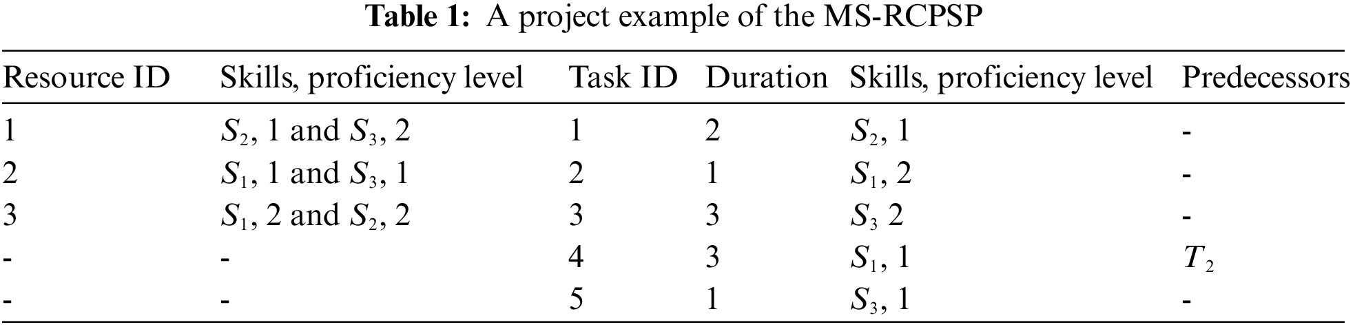
Fig. 1 shows a feasible solution for the project, which will vary in the completion time of the whole project due to the different employees be assigned to task 5. A good dispatching scheme is of great value.

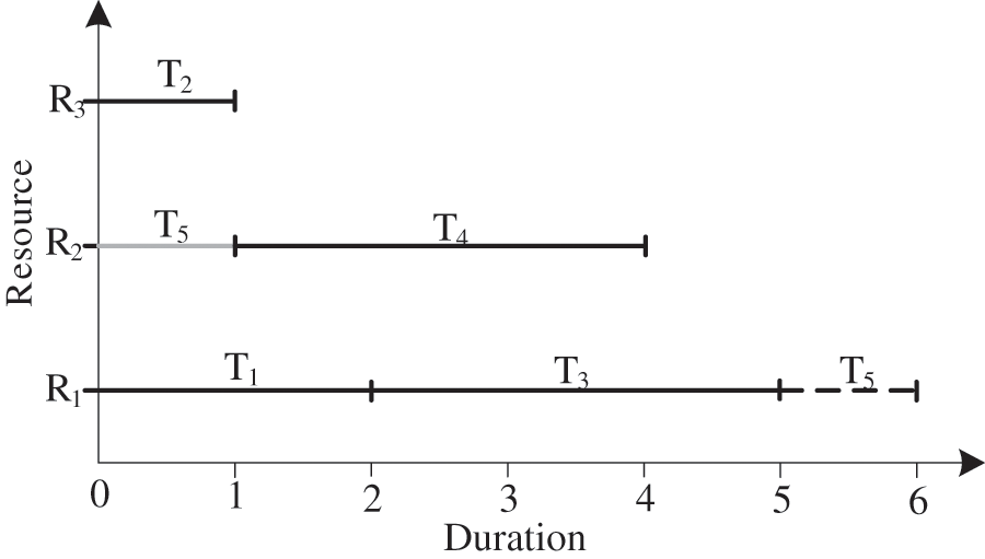
Figure 1: The Gantt chart of a feasible solution

3.2 Dispatching Rules Have Targeted

Dispatching rules have been widely used to solve resource constraints project scheduling problems. However, it is found that few researchers have applied dispatching rules to solve MS-RCPSP. Table 2 shows the Cmax values obtained by four typical dispatching rules for six small-scale MS-RCPSP instances. Each instance has differences in the number of resources, predecessor relationships, and types of skills. The four typical dispatching rules are LPT (longest processing time), SPT (shortest processing time), LRCP (longest of the remaining critical path), and LLFT (latest finishing time).

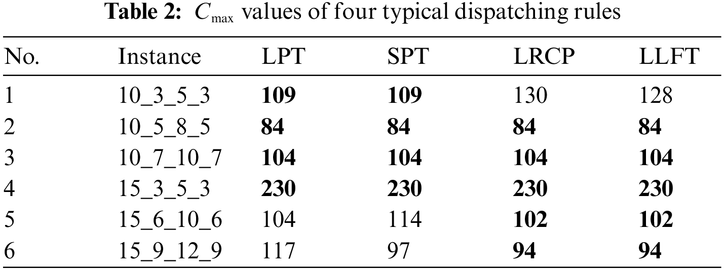
As shown in Table 2, these four dispatching rules obtain the best solution for the instances 10_5_8_5, 10_7_10_7, and 15_3_5_3. But LPT and SPT obtain the best solution for the instance 10_3_5_3. LRCP and LLFT obtain the best solution for the instance 15_6_10_6 and 15_9_12_9. This may be caused by the different inherent properties of each dispatching rule. According to no free lunch, each dispatching rule cannot play the best performance for every instance. Therefore, it is a valuable research direction to explore the newly dispatching rule for this problem.

4  Multi-skill Resource Constrained Project Scheduling Problem

4.1 Problem Description

The Multi-skill resource-constrained project scheduling problem can be described as a project which contains a task set T = {0, 1, 2, …, J, J + 1}. Each task j (j = 0, 1, 2, …, J, J + 1) has a starting time sj and duration dj. Where tasks 0 and J + 1 are virtual tasks. Virtual tasks with duration dj = 0 represent the first and the last tasks in precedence constraints.

Each task j should be assigned once and can start to be assigned when all its predecessor tasks are finished. These precedence relationships of all tasks are presented as a priority relationship matrix H. Each value Pij (i, j = 0, 1, 2, …, J, J + 1) in the matrix H is a 0–1 value. If task i is the predecessor of task j, Pij is set to 1; otherwise, Pij is set to 0. There are K resources {1, 2, …, K} with N skills {1, 2, …, N}. Gkn (Gkn = 0, 1, …, Q) represents the proficiency level of resource k at skill n. A large Gkn value indicates the high proficient level of resource k at skill n. Each task j consumes a resource k and must satisfy the inequality Gkn ⩾ ηjn, ηjn (ηjn = 0, 1, …, Q) denotes the minimum proficiency level of skill n of resource k when task j is assigned to resource k. Moreover, each resource can be assigned at most one task at a time. This paper aims to minimize the project completion time Cmax.

4.2 Problem Formulation

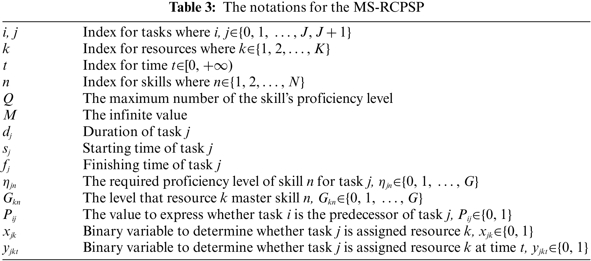
The notations of the MS-RCPSP are shown in Table 3. In this paper, the objective is to minimize the project completion time Cmax, which can be expressed as follows:

minCmax=maxfj,∀j(1)

Temporal constraints: Constraint (2) ensures that each task is continuous and cannot be interrupted. Constraints (3) and (4) ensure that the executed time ranges of each task j in sj to fj, sj, and fj are starting time and finishing time of task j, respectively. Constraint (5) ensures values of the starting time and duration for each task j are a nonnegative number.

fj=sj+dj,∀j(2)

yjktt≥sj,∀j,k,t(3)

yjktt≤fj,∀j,k,t(4)

sj≥0,dj≥0,∀j(5)

Predecessor constraints: If task i is the predecessor task of task j, the starting time sj of task j must not be less than the finishing time fi of task i. It can be expressed as follows:

Pij(sj−fi+1M)>0,∀i,j(6)

Resource constraints: Constraint (7) expresses the proficient level of resource k at skill n must be the required proficiency level of skill n for task j. Constraint (8) ensures each task j only needs one resource. Constraint (9) expresses each resource k can be assigned at most one task at a time.

∑kxjkGkn≥ηjn,∀j,n,k(7)

∑kxjk=1,∀j,k(8)

∑jyjkt≤1,∀j,k,t(9)

Binary variable constraints: There are two binary variables xjkand yjkt. Their ranges of values are shown in Eqs. (10) and (11), respectively.

xjk={ 1,task j is assigned to resource k∀j,k0,other(10)

yjkt={ 1,task j is assigned to resource k at time t∀j,k,t0,other(11)

5  Rules-Mining Framework Using the IGEP Algorithm

GEP is an efficient evolutionary algorithm that inherits the advantages of genetic algorithm (GA) and genetic programming (GP). It has the simplicity of the ‘fixed-length linear string’ of GA, and the searchability of the ‘dynamic tree structure’ of GP. Like GA and GP, the GEP training process includes evolution operators, such as initialization, fitness evaluation, selection, mutation, and crossover (recombination). In addition, GEP has its unique transposition operator, and the rules mining perturbation operator is also designed and added to the IGEP algorithm in this paper. The fitness evaluation process of GEP is similar to that of GP, which is based on the value obtained by converting a binary tree into an ORF expression and then calculating it. The goal of GEP is to find the individual (chromosome) with the highest fitness value.

This paper applies the IGEP algorithm to explore dispatching rules with high fitness to solve MS-RCPSP. The basic idea of the IGEP algorithm is to generate an initial population. Each individual in the population represents a dispatching rule. Then iterate through importing the training set data to evolve the initial population. Each iteration is an evolutionary selection process. Finally, a dispatching rule with high fitness can be obtained.

5.1 Encoding and Decoding

5.1.1 Encoding

The heuristic algorithm based on dispatching rules has the characteristics of simplicity, practicality, and high computing efficiency. Therefore, it is often used to solve resource-constrained project scheduling problems. In the IGEP algorithm, the dispatching rule is used to select a task from the task set πk*, and the set πk* contains all the tasks that can be assigned at the current moment.

This paper extract attributes from Myszkowski et al.’s research [3] and several typical dispatching rules [32,44] to form attribute set V. The elements in set V can be described as follows:

1)   Task duration (pt(j)), it represents the duration of the task j (j = 1, 2, …, J), that is, pt(j) = dj.

2)   The number of immediate predecessor tasks (pn(j)), it represents the number of immediate predecessors of task j.

3)   The number of immediate successor tasks (sn(j)), it represents the number of immediate successors of task j.

4)   The total number of predecessor tasks (pa(j)), it represents the number of total predecessors of task j.

5)   The total number of successor tasks (sa(j)), it represents the number of total successors of task j.

6)   Minimum proficiency level requirements (sg(j)), it represents the minimum proficiency level required for task j.

7)   The remaining critical path length (cpl(j)), it represents the path length with the longest duration in subsequent task paths of task j in the task network diagram.

8)   The number of tasks on the remaining critical path (cpn(j)), it represents the number of tasks on the path with the longest duration in the subsequent task paths of task j in the task network diagram.

9)   The latest finishing time (lf(j)), it represents the latest finishing time of task j.

10)   Slack time (tw(j)), it represents the difference between the latest finishing time lf(j) and the earliest finishing time ef(j) of task j, that is, tw(j) = lf(j) − (es(j) + dj).

11)   The number of optional resources (rn(j)), it represents the number of resources that can be assigned to task j, that is, rn(j)=∑k∈R(Gkn≥njn),∀j,k,n.

The population of the IGEP algorithm is represented as a collection of genotype-encoded individuals, that is, the chromosome with multiple linear strings. This paper defines the attribute set containing V = {pt, pn, sn, pa, sa, sg, cpl, cpn, lf, tw, rn} the above 11 attributes. The function set F = {+, −, *, /, Q, max, min} contains 7 basic function operators.

The encoding process generates an initial population A* with popsize chromosomes. Where popsize is the population size, each chromosome is composed of two parts: the head and the tail. The gene of the head is randomly selected from the function set F and the attribute set V. But the gene of the tail only be chosen randomly from the attribute set V. The length of each chromosome l is determined by the head length h and the maximum number of child nodes mmax of the function operator.

l=h×(mmax+1)−1(12)

Fig. 2 shows an initial population A*, whose population size is popsize = n and the length of head h = 5.

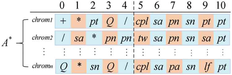
Figure 2: An initial population

5.1.2 Decoding

A feasible solution is usually represented as a genotype-encoded individual. Each chromosome has a corresponding expression tree and ORF expression. As shown in Fig. 3, the chromosome is chrom={+,∗,pt,Q,/,cpl,sa,pn,sn,pt,pt}. Its corresponding expression tree is shown as the binary tree, and its ORF expression is f=cpl×(sa/pn)+pt. The time complexity is O(h), and the space complexity is (h×mmax+1)×mmax=S(h).

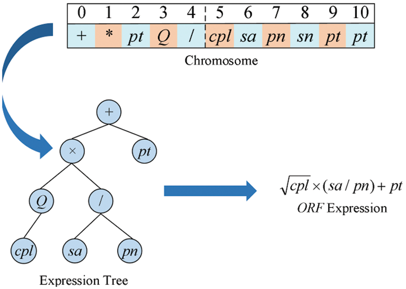
Figure 3: Individual 3 manifestations of basic GEP

In order to reduce the complexity, a backward traversal decoding mechanism is proposed in IGEP. The backward traversal decoding method needs to read the gene of chromosomes one by one. But different from the basic GEP decoding traversal tree building, the backward traversal decoding places the elements in a two-level list before reading the gene. All elements of each sub-list in the list correspond one-to-one with all elements of each depth of the expression tree. The calculation process of backward traversal decoding adopts the calculation-deletion method, that is, the child nodes are deleted when a root node is calculated.

The total time complexity O(h)* of the backward traversal decoding mechanism equals the total time complexity O(h) of the basic GEP decoding process. However, because the elements in the list gradually decrease, the space complexity S(h)* is much smaller than S(h).

Taking a chromosome chrom as an example, its length of chrom is l, and its length of the head is h. i (i = 0, 1, 2, …, l − 1) represents the i-th gene of chrom. Ec and Emare two lists containing contain the same amount of sub-list that stored loci-related information of the effective length Lmax of chrom. The index value of each sub-list corresponds to the tree depth. Pc(j, k) = chrom(i) and Pm(j, k) = mi express chrom(i) and miare the k-th element in the j-th sub-list of list Ec and Emrespectively, which can be expressed as position information of the gene chrom(i), that is, the position in the expression tree is the k-th element with a tree depth of j, and the number of child nodes is mi.

The decoding process of chrom can be shown in the pseudo-code of Procedure 1, which adopted the breadth-first approach.

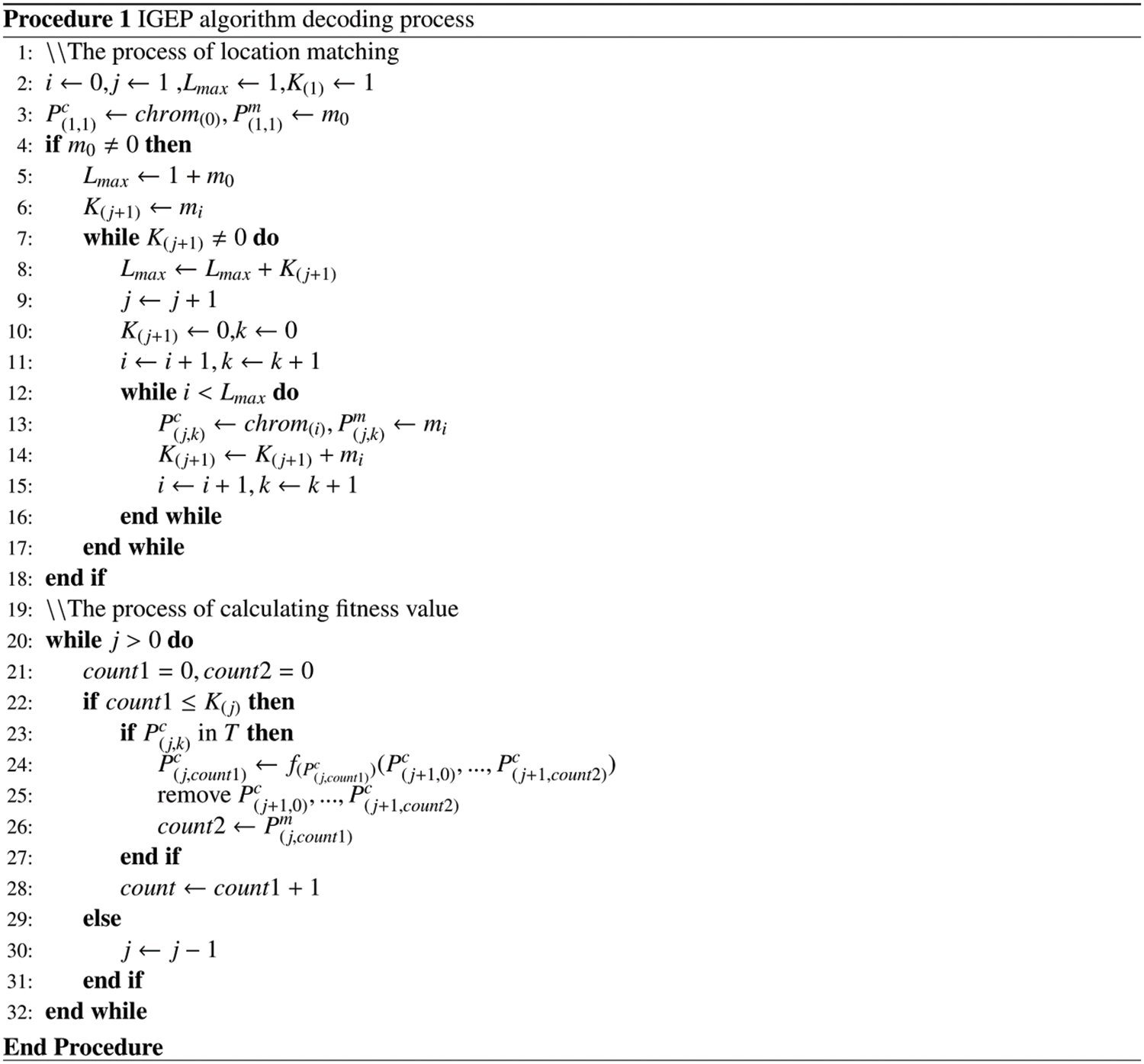
The decoding procedure of the IGEP algorithm is shown in Procedure 1. K(j+1) represents the number of elements with a depth of j + 1 in the expression tree. count1 is the count of the depth of the current element in the calculation process. count2 is a count used to match the expression tree position of each function’s child node. When the function value of a root node is calculated each time, the child node corresponding to the root node is also deleted. The next depth’s first element corresponds to each root node’s first root node in the current depth. f(PC(j,count1)) is the function expression corresponding to the root node. (Pc(j+1, 0), …, Pc(j+1, count2)) is the parameter value set of all branch nodes corresponding to f(PC(j,count1)). The calculation process of function value is a process of gradually evaluating from the maximum depth to the minimum depth of the root node, then replacing the original function symbol of the node with the function value. It is used as the input parameter value of the function expression corresponding to a root node of the previous depth. Finally, the value of the initial root node Pc(1, 1) is equal to the value calculated by the ORF expression of chrom and is used as the priority value of the task.

The decoding process has the prototype of the building expression tree. It is only necessary to substitute each element Pc(j, k) in the traversed list Ec into the k-th node of the tree depth j. Connecting nodes of adjacent depths according to the value of Pm(j, k), an expression tree can be drawn.

5.2 Evolutionary Approach

The main idea of the IGEP algorithm is as follows. First, the initial population is randomly generated. Then, the population evolved. Finally, an optimal chromosome is obtained, that is, an optimal dispatching rule. In the iterative process, the IGEP algorithm adopts several evolution operators: selection and replication, perform mutation operation, IS-transposition, RIS-transposition, one-point crossover, and two-point crossover [36]. In addition, the rule mining perturbation mechanism is added to avoid falling into the local optimum.

S1: selection and replication. The IGEP algorithm uses the roulette selection method. Based on the fitness values of chromosomes in population A, a new population Anew with the same scale as population A is generated. Chromosome with high fitness values in A is more likely to appear in Anew. Chromosomes with high fitness values usually appear multiple times in Anew to replace chromosomes with low fitness values in population A.

S2: rule mining disturbance operation. According to the preset rule mining perturbation preset value d_value, the rule mining perturbation mechanism is triggered if the historical optimal individual chrom*best does not change within d_value iterations. The perturbed chromosome is selected by a certain perturbation probability. The rule mining perturbation mechanism can effectively break the local optimum and enrich the gene types in population A.

S3: perform mutation operation. The mutation operation is a very common evolutionary operator in the intelligent evolutionary algorithm. The mutation operation refers to selecting a chromosome from population A by a certain mutation probability. A gene chrom(a) is randomly selected and replaced by a random element in function set F or attribute set V. If chrom(a) is a tail gene, the only element in the attribute set V can be selected for replacement.

S4 and S5: IS-transposition and RIS-transposition. Both an insertion sequence transposition (IS-transposition) and a root insertion sequence transposition (RIS-transposition) select chrom by a certain probability. Then two gene positions a and b are randomly selected, and a head gene position c is randomly selected. The gene fragment {chrom(a), chrom(a+1), …, chrom(b)} are copied and inserted into the front of gene position c. Meanwhile, all the head genes after position c move backward in turn. If the gene’s position exceeds the head, the gene should be discarded. The difference between IS-transposition and RIS-transposition lies in the position of c. The head gene position c of the IS-transposition in any position in the head except the first position.

S6 and S7: one-point crossover and two-point crossover. The crossover operator refers to selecting two parents (chrom1 and chrom2) from population A. In the one-point crossover operation, a position a is chosen randomly. Then two gene fragments {chrom1(0), chrom1(1), …, chrom1(a)} of chrom1 and {chrom2(0), chrom2(0), …, chrom2(a)} of chrom2 are swapped. For the two-point crossover operation, two positions a and b are randomly selected. Then two gene fragments {chrom1(a), chrom1(a+1), …, chrom1(b)} of chrom1 and {chrom2(a), chrom2(a+1), …, chrom2(b)} of chrom2 are swapped. Two new chromosomes chrom1new and chrom2new will be obtained after a one-point crossover or two-point crossover. The parent chromosomes chrom1 and chrom2 will be replaced with chrom1new and chrom2new.

5.3 Evaluation Function

The objective is to obtain the minimum project completion time minCmax of MS-RCPSP. During the fitness evaluation process, the project completion time of all instances is calculated as the fitness value fi of chromosome i in population A. The fitness value fi uses the relative deviation calculation method and is calculated as follows:

fi=∑j=1Ci(M−|C(i,j)−T(j)T(j)×100|)(13)

In Eq. (13), M refers to the upper limit of the fitness value. C(i,j) refers to the Cmax value of the instance j in the i-th chromosome. Because the lower bound of Cmax cannot be obtained, an unsupervised learning method is used. In Eq. (13), T(j) is a variable that represents the historical optimal project completion time of instance j. It is used to evaluate the fitness value of each individual in population A.

5.4 Feasible Solution Generation

Combined dispatching rules with the parallel scheduling mechanism, a fixed scheduling scheme will be obtained for each instance. Therefore, the specific scheduling process in IGEP does not need to compile the string encoding. The priority value of each task is determined by the dispatching rule and its attributes. Then, a scheduling scheme and the Cmax value are obtained.

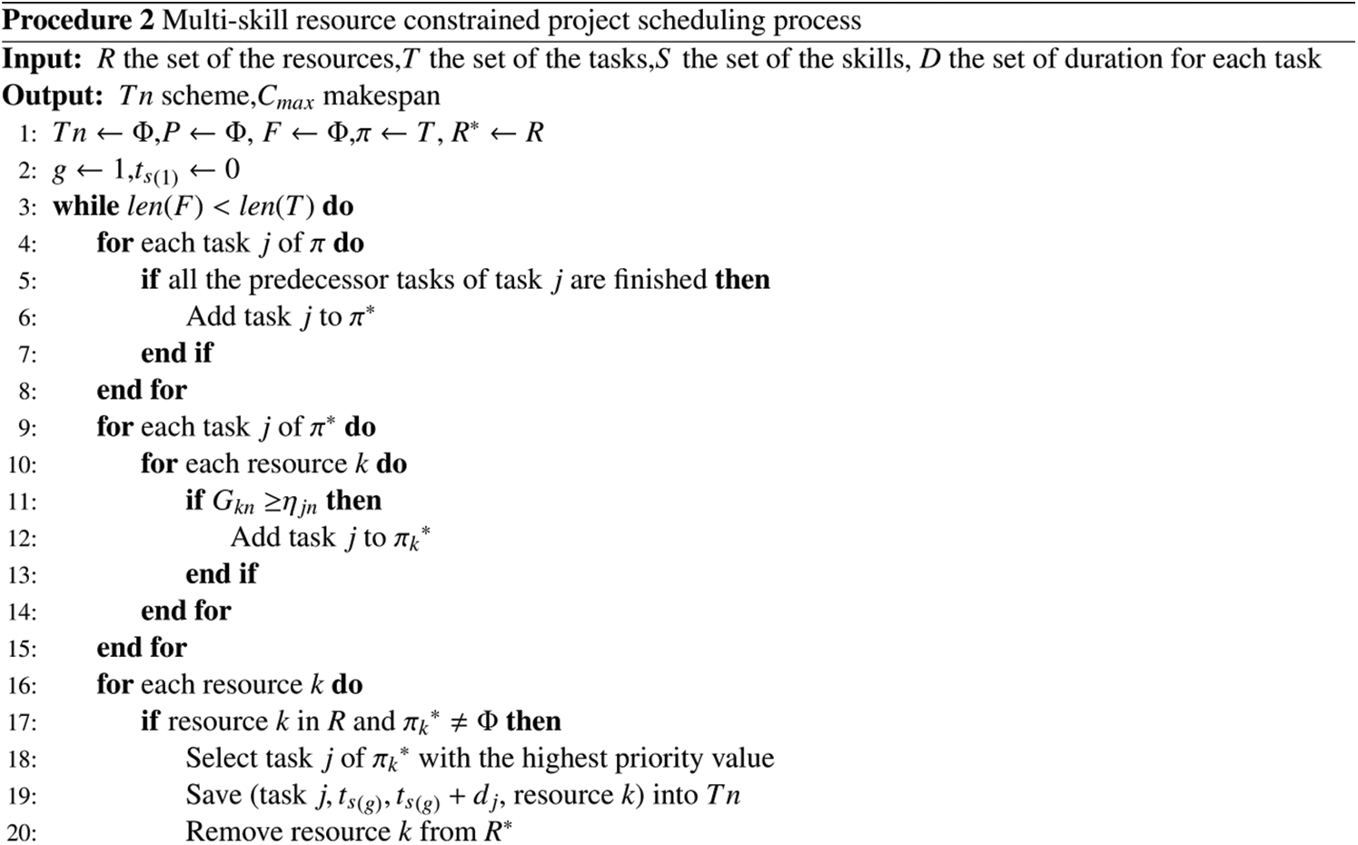
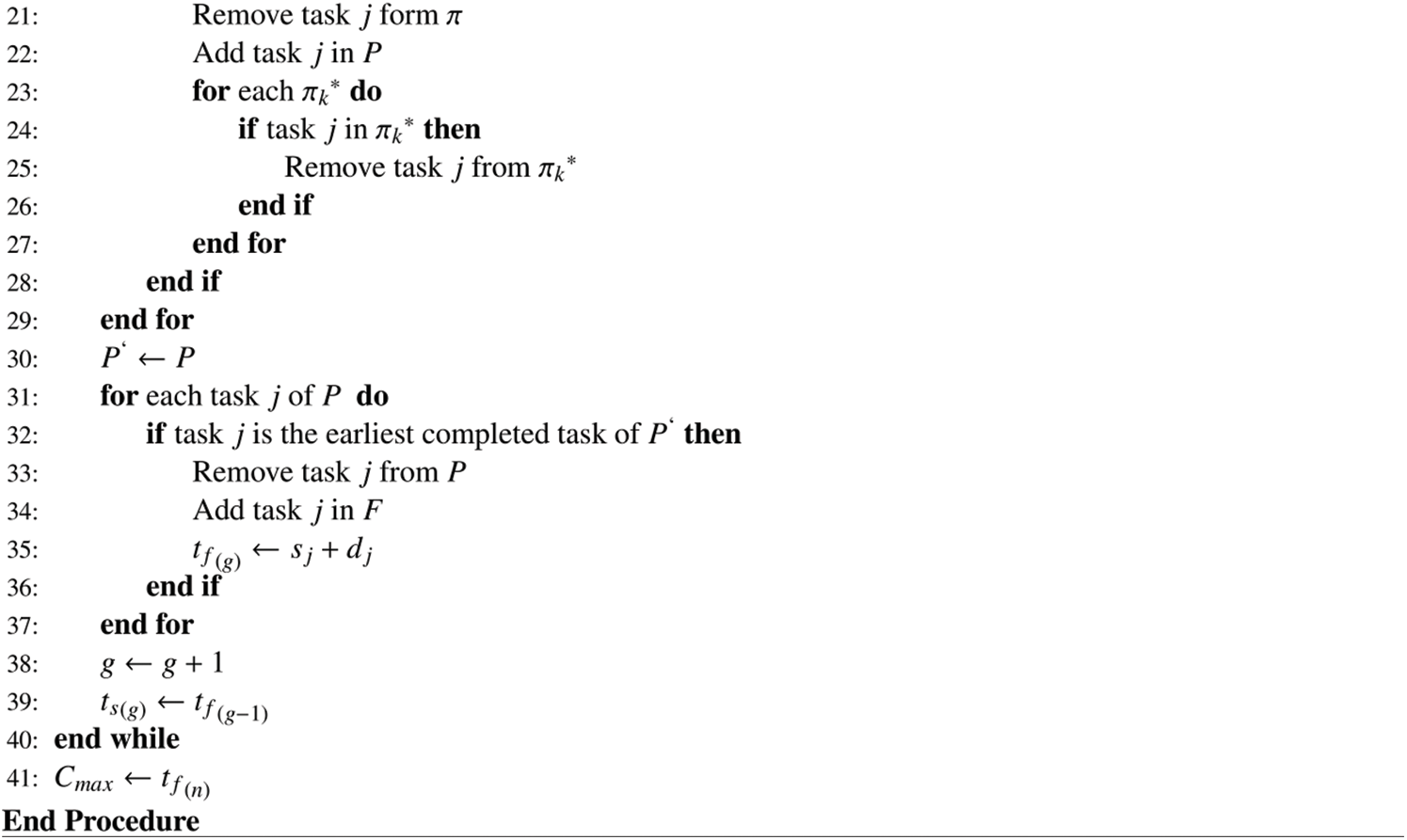
Procedure 2 is the pseudo-code of the scheduling process for the multi-skill resource-constrained project scheduling problem. The scheduling process adopts a parallel scheduling mechanism and divides the entire scheduling process into g stages. The starting time of the first stage is set to ts(1) = 0. The starting time of each stage is equal to the finishing time of the previous stage, that is, ts(g) = tf(g−1).

Firstly, according to the predecessor constraints and resource constraints, all tasks that can be allocated are selected from the unallocated task set π, , and stored in the optional task set π* of the current stage. If task j from π* can be executed by the idle resource k, task j is stored in the set πk*(k = 1, 2, …, K) when Gkn ≥ njn. Then, if task j is in πk* with the highest priority value, the idle resources k should be assigned to task j. It should be noted that each task can be assigned to exactly one resource and can only be assigned once. Finally, the finishing time tf(g) of each stage is determined by the completion time of the earliest completed task j in each stage, where tf(g) = sj + dj. Multiple tasks may be completed simultaneously. The completion time Cmax is the finishing time of the last stage. A feasible scheduling scheme Tn can be obtained.

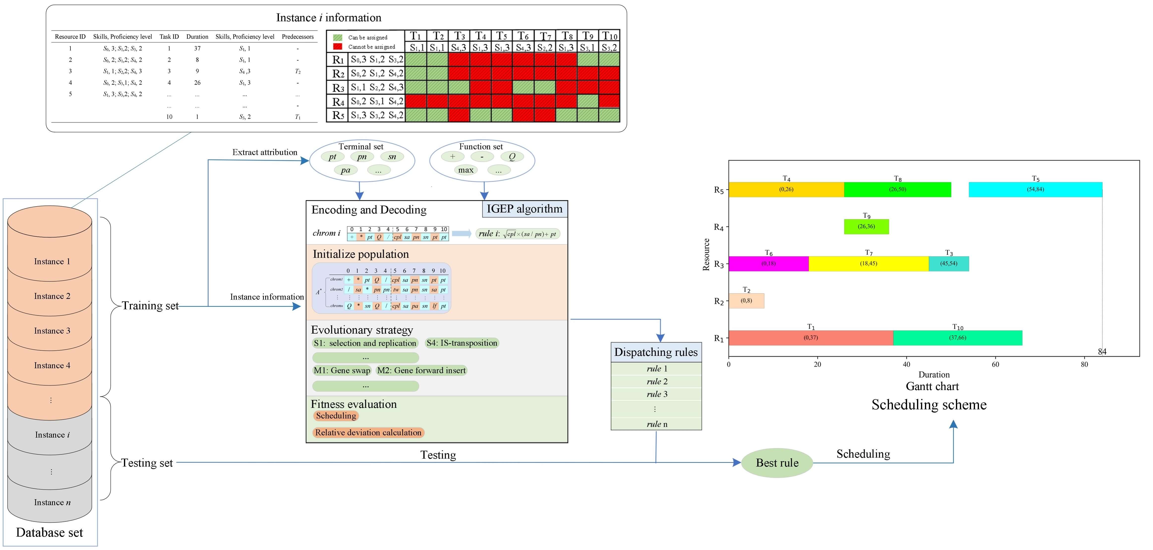
Taking the example 10 * 5 * 7 * 5 as an example, the project resource task relationship matrix is shown in Fig. 4. From Fig. 4, it can be seen which resources can meet the skill requirements of the task and which tasks can be assigned to the resources. For example, these resources selected by task 1 are {R1, R2, R3, R5}. Resource 3 can only execute task 3. The Gantt chart can be obtained as shown in Fig. 5.

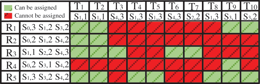
Figure 4: The skill matrix of the instance 10 * 5 * 7 * 5

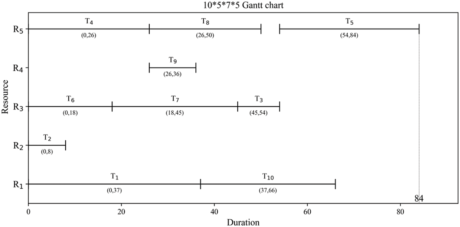
Figure 5: The Gantt chart of instance 10 * 5 * 7 * 5

Fig. 5 shows the starting time, the finishing time, the resource selection of each task, and so on. The project completion time is 84.

5.5 Neighborhood Structures

An efficient neighborhood structure will significantly improve the performance of the IGEP algorithm. Six neighborhood structures {M1, M2, M3, M4, M5, M6} are proposed. The detail flowchart of six neighborhood structures in Fig. 6.

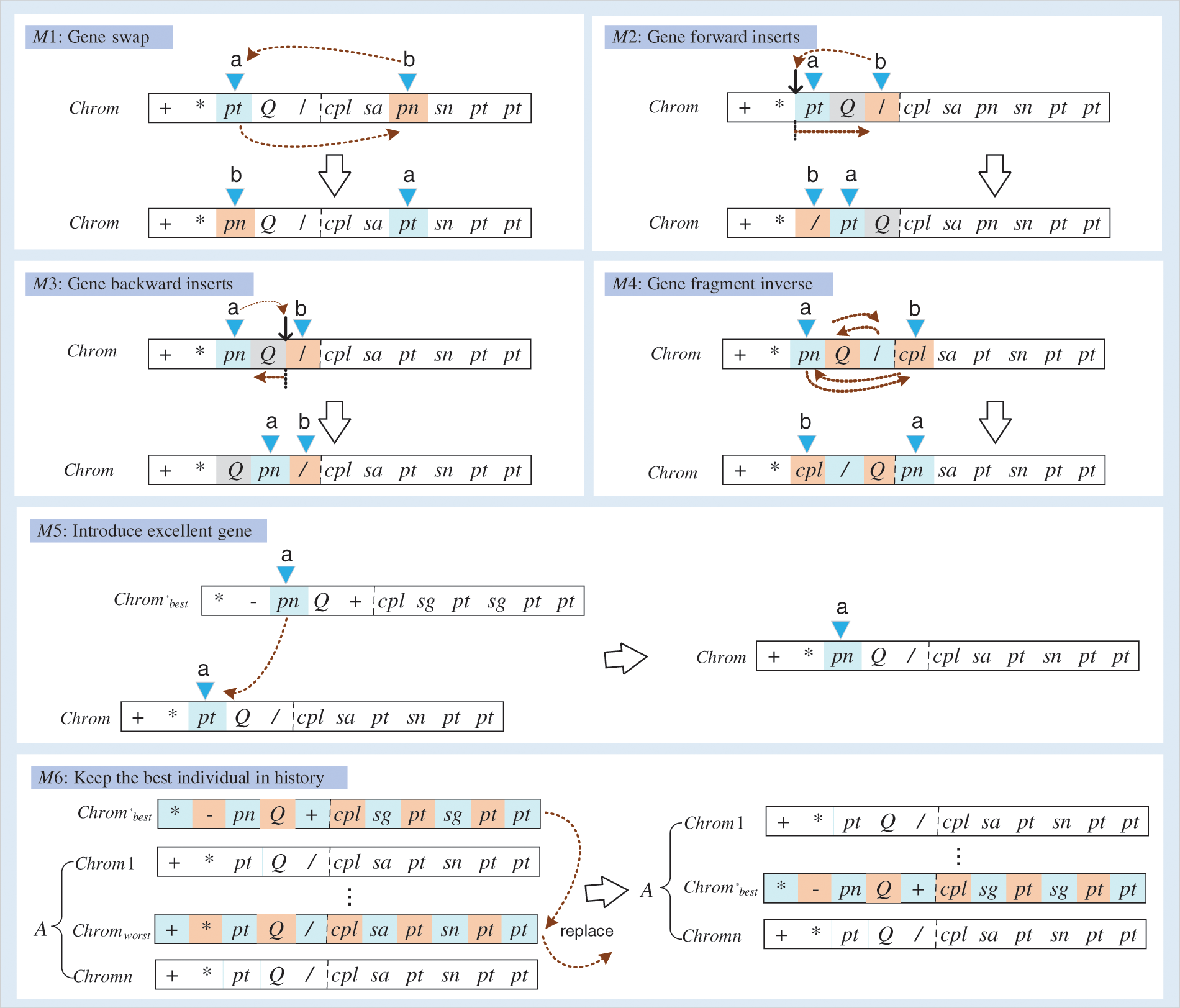
Figure 6: The flowchart of six neighborhood structures

Gene swap (M1): A chromosome chrom is selected by a certain probability. Then two different genes (chrom(a) and chrom(b)) are randomly chosen from chrom to swap. Note: To avoid the generation of illegal chromosomes, it is necessary to limit position b. If chrom(a) is an element from the function set F, then chrom(b) can only be selected from individual head genes; otherwise, chrom(b) is selected from the non-functional genes of the chromosome.

Gene forward inserts (M2): A chromosome chrom is selected by a certain probability. Then two genes (chrom(a) and chrom(b)) are randomly selected from chrom. The latter gene chrom(b) is inserted in front of the former gene chrom(a). Note: chrom(a) and chrom(b) both are not the first gene in chrom. Meanwhile, to avoid the generation of illegal chromosomes, if chrom(a) is the gene at head positions, and the last gene at the head position is an element from the function set F, then chrom(b) can only select the gene from head positions.

Gene backward inserts (M3): A chromosome chrom is selected by a certain probability. Then two genes (chrom(a) and chrom(b)) are chosen randomly. The former gene chrom(a) is inserted in front of the latter gene chrom(b). Note: chrom(a) and chrom(b) both are not the first gene in chrom. Meanwhile, to avoid the generation of illegal chromosomes, if chrom(a) is the gene at head positions, then chrom(b) can only select the gene from head positions.

Gene fragment inverse (M4): A chromosome chrom is selected by a certain probability. Then two genes (chrom(a) and chrom(b)) are chosen randomly. All genes {chrom(a), chrom(a+1), …, chrom(b)} are updated in reversed order. Note: To avoid the generation of illegal chromosomes, if chrom(a) is the gene at head positions, then chrom(b) can only select the gene from head positions.

Introduce excellent gene (M5): A chromosome chrom is selected by a certain probability. Then a gene position a is randomly selected. The gene chrom(a) is replaced by chrom*best(a) from the historical optimal individual chrom*best. A new chromosome chromnew is generated. If the fitness value of chromnew is higher than that of chrom, then replace the chrom in the population with chromnew.

Keep the best individual in history (M6): If the historical optimal chromosome is not in the population, the worst chromosome chromworst is replaced by the historical optimal chromosome chrom*best.

5.6 IGEP Framework

The proposed IGEP algorithm can be roughly divided into four steps. The first step is to determine the elements of the function set and terminal set, and to set parameter values, such as chromosome length, mutation probability, etc. The second step is to divide the data set into the training set and testing set with a ratio of 2:3. The third step is to train the best individual by the training set data. The fourth step is to use the testing set data to test the performance and verify the performance of the IGEP algorithm. Fig. 7 shows the flowchart of the IGEP algorithm.

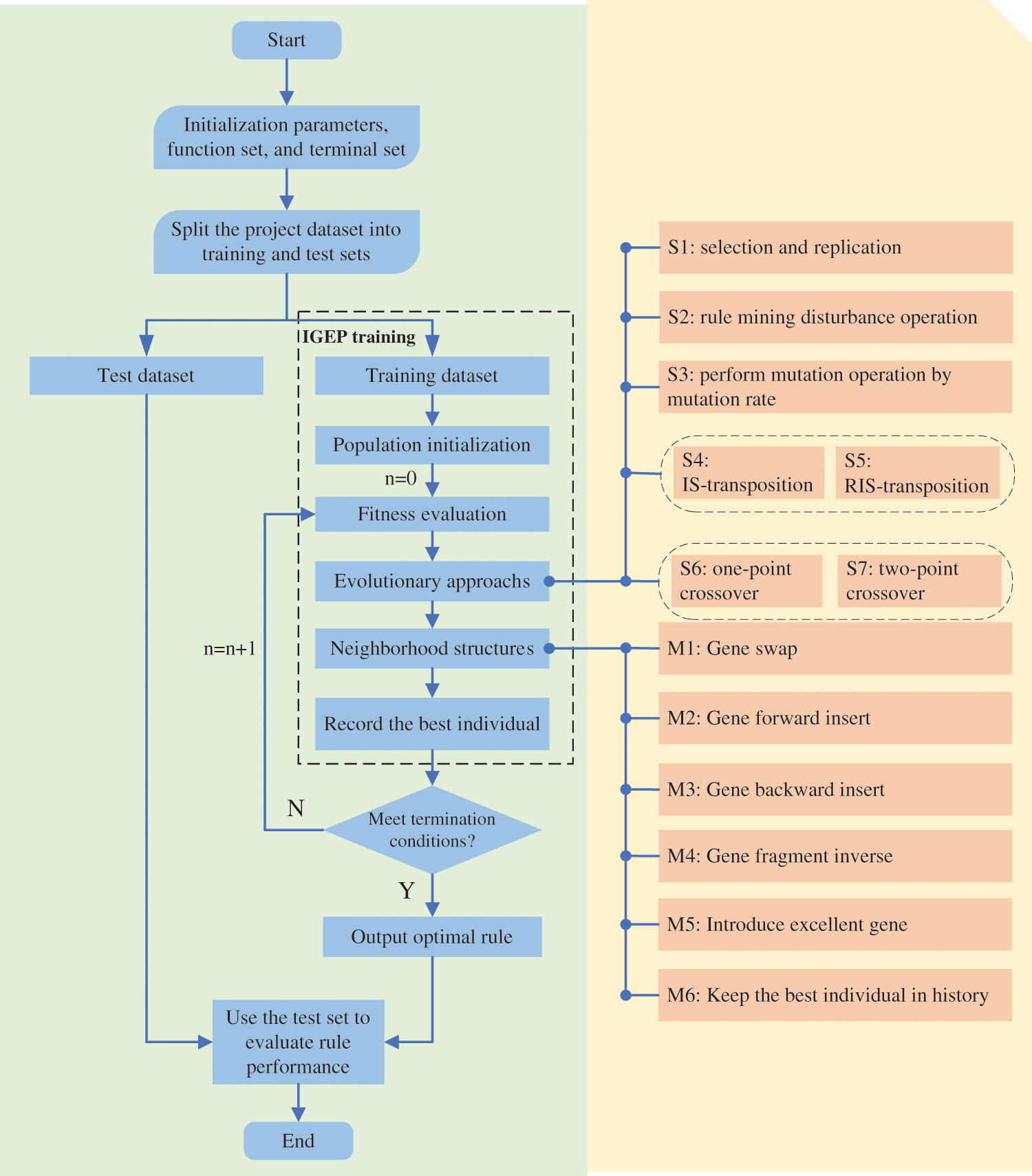
Figure 7: The flowchart of the IGEP algorithm

6  Computational Results and Analysis

To evaluate the performance of the IGEP algorithm, the benchmark case set (iMOPSE) created by Myszkowski et al. [2] in 2015 is adopted. The iMOPSE contains 36 instances. The IGEP algorithm is implemented in Python 3.10 and operated on a core R7-5800H processor with 3.3 GHz and 16 GB RAM.

6.1 Parameter Setting

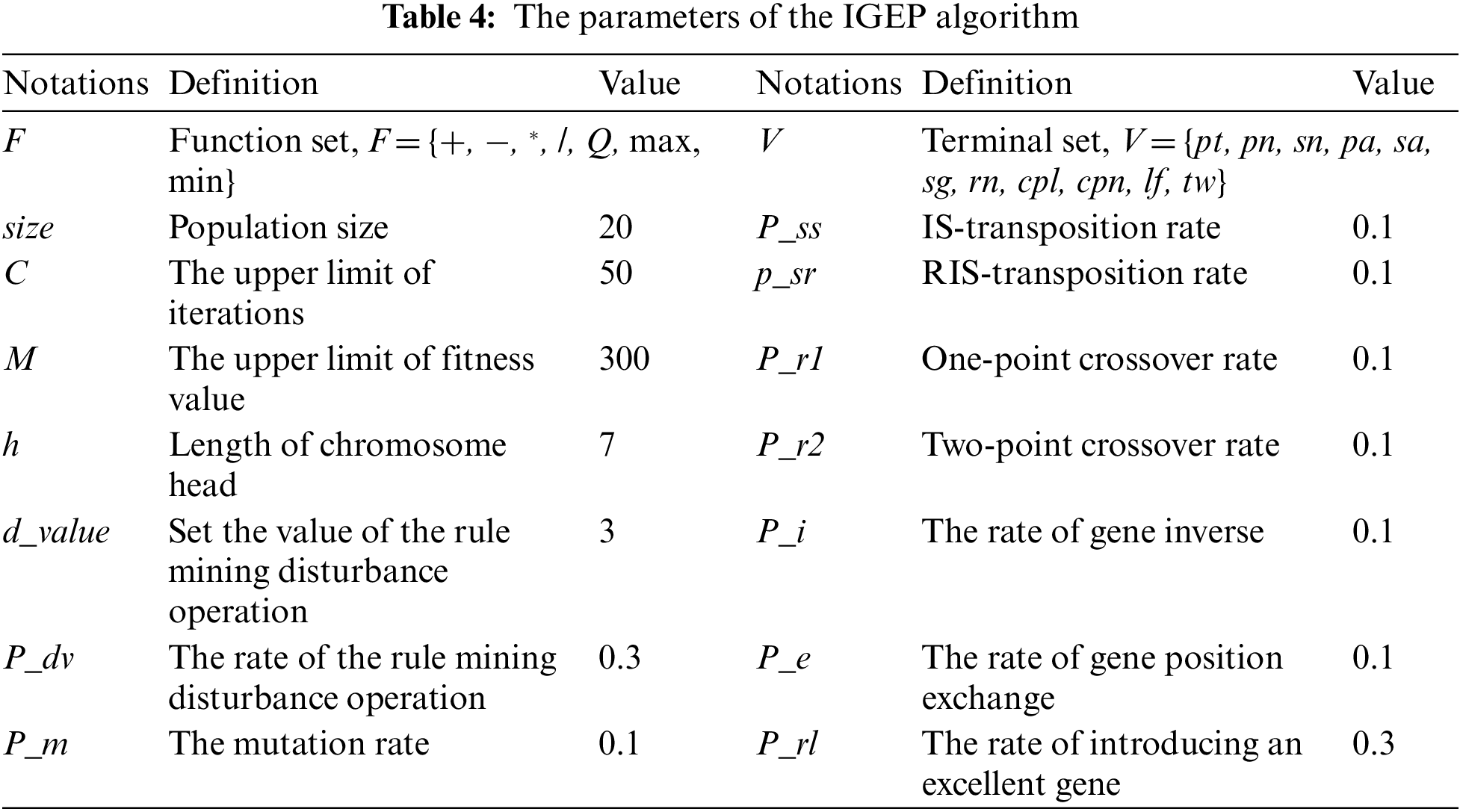
In this section, the parameters are determined. The proposed IGEP algorithm with the long length of the head is easier to obtain excellent dispatching rules. But the computational complexity will increase significantly. After a series of experiments, when the length of the head h is equal to 7, the proposed IGEP algorithm can maintain superior performance and low computational complexity. Otherwise, the parameters such as population size, number of iterations, the preset value of rule mining disturbance, preset probability of rule mining, and mutation rate also significantly impact the performance of the proposed IGEP algorithm.

Before the experiment, the results of IGEP algorithm under different combination of numerical parameters were compared. The comparative method adopts the calculation of relative deviation. The group of parameters with the smallest relative deviation value was selected as the input parameters of the experiment. The parameters of the IGEP algorithm are listed in Table 4.

To illustrate the performance of the newly dispatching rule generated by the IGEP algorithm, this paper selects six relatively typical dispatching rules. These six dispatching rules are described as follows:

1)   Shortest processing time priority rule (SPT) [45], this dispatching rule takes the task duration pt as the evaluation criterion. The smaller pt value means the higher priority of the task. It is a typical dispatching rule based on the project network.

2)   Longest processing time priority rule (LPT) [45], this dispatching rule is the opposite of the SPT rule. The task with a large pt value has a higher priority.

3)   Longest of the remaining critical path priority rule (LRCP) [46], this dispatching rule only considers the task’s remaining critical path length cpl value. And the task with a large cpl value has a higher priority.

4)   Minimum slack time priority rule (MINSLK) [44]. In this rule, the slack time tw of the task is taken as the evaluation criterion. The task with a smaller tw value is given a higher priority.

5)   Latest finishing time priority rule (LLFT), it considers the value of the task’s latest finishing time lf. The purpose is to assign tasks with smaller lf values as early as possible.

6)   The most number of immediate successors priority rule (MIS) [44], this rule gives a higher priority to a task with a large number of immediate tasks. A task with a large sn value has a higher priority.

According to different factors considered, dispatching rules can be roughly divided into four types, such as project network-based dispatching rules (NBR), critical path-based dispatching rules (CPBR), resource-based dispatching rules (RBR), and hybrid dispatching rules (CR) [44]. The SPT rule, the LPT rule, and the MIS rule are the project network-based dispatching rules. The LRCP rule, the MINSLK rule, and the LLFT rule are critical path-based dispatching rules.

6.2 The iMOPSE Benchmark Dataset

The iMOPSE benchmark dataset is selected for multi-skill resource-constrained project scheduling problem research. The dataset contains 36 instances with 100 or 200 tasks and 5, 10, 20, or 40 resources. The number of skill types is 9, 14, or 15. The dataset was created by Myszkowski et al. [2] in 2015 and can be found on website http://imopse.ii.pwr.edu.pl.

6.3 The Discovered Dispatching Rules via IGEP

The purpose of the IGEP algorithm in this paper is to explore the optimal dispatching rule for solving the multi-skill resource-constrained project scheduling problem. According to the approximate ratio of 2:3, 16 instances are randomly selected as the training set. The remaining 20 instances are the testing set. The training set is used to discover the optimal dispatching rule during the exploration of the IGEP algorithm. The testing set is used to verify the performance of the optimal dispatching rule.

Fig. 8 shows ten discovered dispatching rules under 10 independent runs of the proposed IGEP algorithm. Eight discovered dispatching rules positively correlate with the remaining critical path length cpl. Six discovered dispatching rules positively correlate with the maximum skill level requirement sg. This means that the task with large cpl and sg has priority to be allocated resources and to be started.

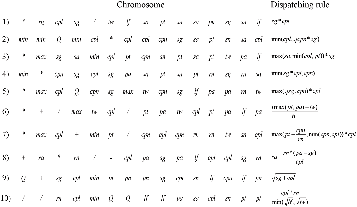
Figure 8: Ten discovered dispatching rules acquired from 10 independent runs

It can be seen from the 10 new dispatching rules that pn and sn are completely lost. By analyzing the case set data, it is found that all tasks have only one direct predecessor task, and the number of direct successor tasks of most tasks is 0 after statistics. In addition, pa and sa have poor performance in 10 new dispatching rules. However, both sg and cpl have achieved good performance. Therefore, it is bold to make an assumption that the relatively simple predecessor relation network of the case leads to poor performance of the attributes related to the predecessor relation network, which is gradually replaced by the attribute values related to duration in the iterative process.

6.4 Comparison among Ten Discovered Dispatching Rules

One-way analysis of variance (ANOVA) was used to analyze the statistical differences in the performance of 10 dispatching rules. The actual project completion time Cmax has significant differences. Therefore, the experiment uses the relative percentage deviation (RPD) to measure the performance of 10 discovered dispatching rules. The computational formula of RPD is shown in expression (14).

RPDj,i=Cj,i−minCjmaxCj−minCj×100%(14)

where Cj,i represents the Cmax value of the instance j via the dispatching rule i. MaxCmax and minCmax represent the maximum Cmax value and minimum Cmax value of instance j via all dispatching rules, respectively. RPDj,i is the RPD value of instance j via dispatching rule i. In the one-way ANOVA of this experiment, the single factor refers to the discovered dispatching rules. The response variable is the RPD value. The ANOVA results are shown in Table 5.

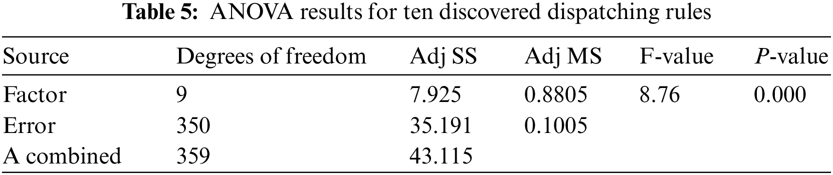
It can be seen from Table 5 that the P-value is approximately 0. Hence, all dispatching rules have statistical differences. This shows that the performance of the ten dispatching rules is significantly different. The pairwise multiple comparisons display the detailed differences among ten dispatching rules and find the high-quality ones, as shown in Fig. 9. Fig. 9 shows the difference in the performance of each discovered dispatching rule.

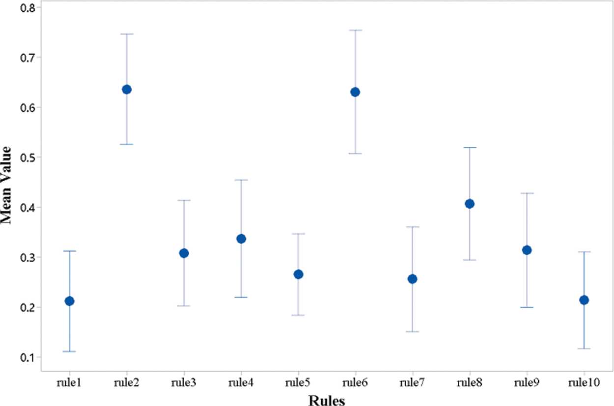
Figure 9: Pairwise multiple comparisons for ten discovered dispatching rules

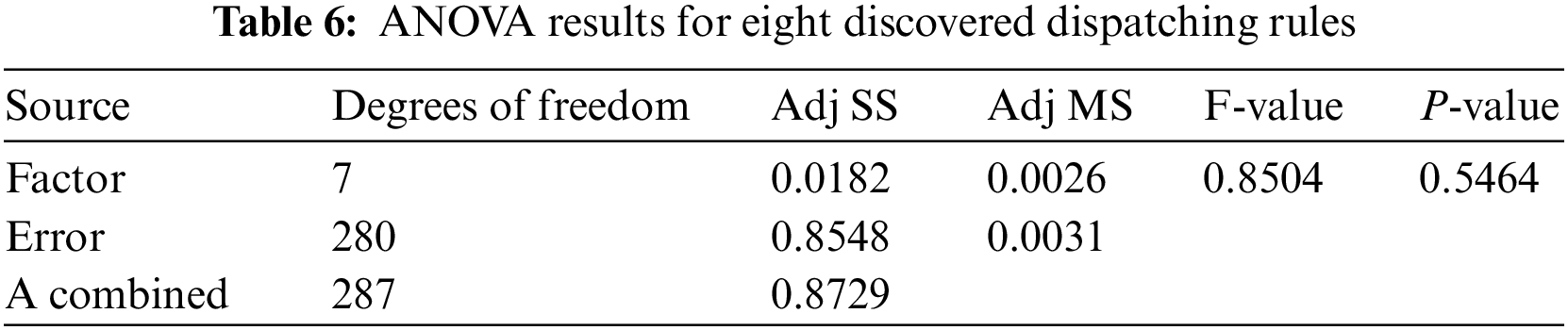
It can be seen that the group means of rule1 and rule10 are significantly better than the group means of other discovered dispatching rules in Fig. 9. The group means of rule3, rule4, rule5, rule7, rule8, and rule9 are smaller than the group means of rule1 and rule10. The group means of rule2 and rule6 are significantly larger than the group means of the other eight discovered dispatching rules. The mean value of RPD for ten discovered dispatching rules are 0.211, 0.636, 0.308, 0.336, 0.265, 0.63, 0.255, 0.406, 0.313, 0.213. The rule1 with 0.211 mean value of RPD is the best discovered dispatching rule. Meanwhile, the mean value of RPD of rule3, rule4, rule5, rule7, rule8, rule9, and rule10 is the closest dispatching rule to rule1. To verify the statistical performance of these eight discovered dispatching rules, One-way analysis of variance (ANOVA) is used to analyze the performance of rule1, rule3, rule4, rule5, rule7, rule8, rule9, and rule10. To verify the statistical performance of these eight discovered dispatching rules, One-way analysis of variance (ANOVA) is used to analyze the performance of rule1, rule3, rule4, rule5, rule7, rule8, rule9, and rule10. As can be seen in Table 6, the P-value exceeds 0.5. Therefore, this difference was not statistically significant for rule1, rule3, rule4, rule5, rule7, rule8, rule9, and rule10.

6.5 Comparison with the Typical Dispatching Rules

In order to verify the effectiveness and excellent performance of the IGEP algorithm, eight discovered dispatching rules are compared and analyzed with six typical dispatching rules. Table 7 shows the comparison results of the completion time Cmax and the relative percentage deviation value RPD among the above-mentioned dispatching rules.

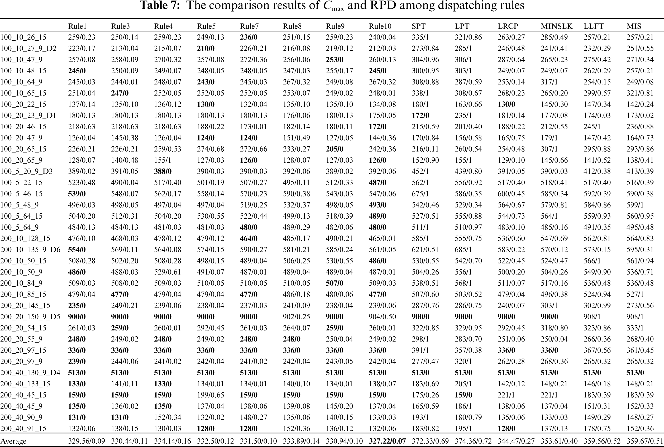
It can be seen from Table 7, eight discovered dispatching rules obtain the best Cmax than six typical dispatching rules. 14, 12, and 12 instances of rule1, rule7, and rule10 obtained the best Cmax, respectively. Six typical dispatching rules with a single attribute have a bad performance. The LRCP rule is the best one among the six typical dispatching rules. In sum, the discovered dispatching rules play a good performance in solving MS-RCPSP problem.

To further study the differences in the performance of the dispatching rules, a one-factor analysis of variance (ANOVA) is performed on 36 instances. The single factor refers to the fourteen dispatching rules. The response variable is the RPD value. The ANOVA results are shown in Table 8.

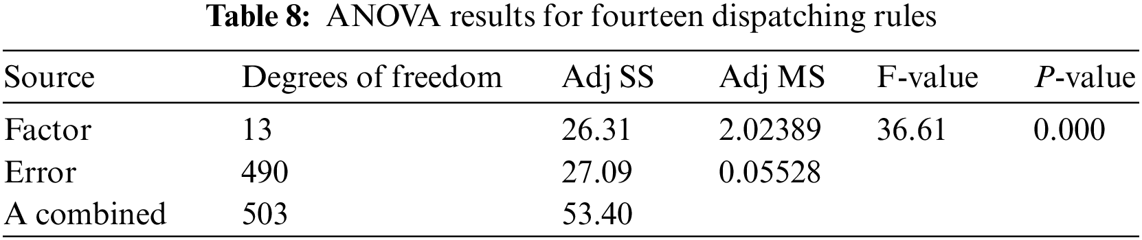
The ANOVA result in Table 8 shows that the P-value is close to 0. This indicates that the statistical performance of the fourteen dispatching rules is significantly different. To clearly show the difference among those dispatching rules, the mean square error control chart is applied to describe the difference, as shown in Fig. 10.

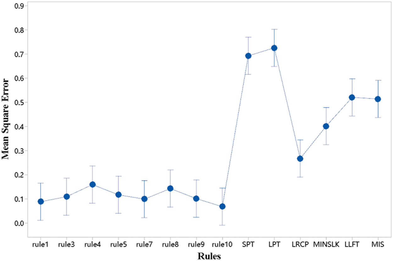
Figure 10: Mean square error control chart

Fig. 10 shows the mean square error values of fourteen dispatching rules, which are 0.088, 0.109, 0.159, 0.117, 0.099, 0.143, 0.101, 0.068, 0.692, 0.725, 0.267, 0.401, 0.52, and 0.514, respectively. rule10 with the smallest mean square error is the best dispatching rule, followed by rule1 and rule7. These mean square error values of eight dispatching rules mined by the IGEP algorithm are much smaller than that of six typical dispatching rules. It demonstrates that the dispatching rule trained by the IGEP algorithm is much better than typical dispatching rules for solving MS-RCPSP.

7  Conclusion and Future Research

For solving the multi-skill resource-constrained project scheduling problem (MS-RCPSP), this paper constructs a mix-integer mathematical model and proposes an improved gene expression programming algorithm (IGEP) with a backward traversal decoding mechanism to explore the newly dispatching rules. These newly dispatching rules can easily be applied to the real project and production environment. The experimental analysis shows that the newly discovered dispatching rules play a better performance than the typical dispatching rules. This illustrates that the proposed IGEP algorithm with the merit of artificial intelligence and unsupervised learning is effective in exploring the newly dispatching rules for solving the MS-RCPSP problem. Compared with complex real project scenarios and existing research, there are many research directions that are worthy of in-depth study in future research.

1)   The skill proficiency of a resource grows with the long operations, which can increase productivity, and the resource can perform the more demanding tasks. Thus, adding learning mechanisms to resources is closer to some realistic production and maintenance scenarios.

2)   A reasonable resource allocation plan can result in significant cost savings in real project scenarios. Therefore, having a reasonable resource allocation plan while ensuring the project completion time is a direction well worth our research.

Funding Statement: This paper presents work funded by the National Natural Science Foundation of China (Nos. 51875420, 51875421, 52275504).

Conflicts of Interest: The authors declare that they have no conflicts of interest to report regarding the present study.

References

1. Lin, J., Zhu, L., Gao, K. Z. (2020). A genetic programming hyper-heuristic approach for the multi-skill resource constrained project scheduling problem. Expert Systems with Applications, 140. https://doi.org/10.1016/j.eswa.2019.112915 [Google Scholar] [CrossRef]
2. Zhang, Z. K., Tang, Q. H., Chica, M. (2021). A robust MILP and gene expression programming based on heuristic rules for mixed-model multi-manned assembly line balancing. Applied Soft Computing, 109, 107513. https://doi.org/10.1016/j.asoc.2021.107513 [Google Scholar] [CrossRef]
3. Myszkowski, P. B., Skowroński, M. E., Sikora, K. (2015). A new benchmark dataset for multi-skill resource-constrained project scheduling problem. Proceedings of the 2015 Federated Conference on Computer Science and Information Systems, pp. 129–138. Lodz, Poland. https://doi.org/10.15439/2015F273 [Google Scholar] [CrossRef]
4. Myszkowski, P. B., Siemieński, J. J. (2016). GRASP applied to multi–skill resource–constrained project scheduling problem. Department of Computational Intelligence, Wroclaw University of Technology, Wroclaw, Poland. https://doi.org/10.1007/978-3-319-45243-237 [Google Scholar] [CrossRef]
5. Dziwiñski, P., Bartczuk, Ł (2020). A new hybrid particle swarm optimization and genetic algorithm method controlled by fuzzy logic. IEEE Transactions on Fuzzy Systems, 28, 1140–1154. https://doi.org/10.1109/TFUZZ.2019.2957263 [Google Scholar] [CrossRef]
6. Li, L., Tang, Q. H., Zheng, P., Zhang, L. P. (2016). An improved self-adaptive genetic algorithm for scheduling steel-making continuous casting production. Proceedings of the 6th International Asia Conference on Industrial Engineering and Management Innovation, pp. 399–410. Tianjin, China. https://doi.org/10.2991/978-94-6239-148-2_40 [Google Scholar] [CrossRef]
7. Li, D., Zhang, D. D., Zhang, N., Zhang, L. P. (2022). A novel hybrid algorithm for scheduling multipurpose batch plants. Computer Aided Chemical Engineering, 51, 961–966. https://doi.org/10.1016/B978-0-323-95879-0.50161-2 [Google Scholar] [CrossRef]
8. Huang, R. X., Ning, J. Y., Mei, Z. H., Fang, X. D., Yi, X. M. et al. (2021). Study of delivery path optimization solution based on improved ant colony model. Multimedia Tools and Applications, 80, 28975–28987. https://doi.org/10.1007/s11042-021-11142-1 [Google Scholar] [CrossRef]
9. Guan, B. X., Zhao, Y. H., Li, Y. (2021). An improved ant colony optimization with an automatic updating mechanism for constraint satisfaction problems. Expert Systems with Applications, 164, 114021. https://doi.org/10.1016/j.eswa.2020.114021 [Google Scholar] [CrossRef]
10. He, M. L., Wei, Z. X., Wu, X. H., Peng, Y. T. (2021). An adaptive variable neighborhood search ant colony algorithm for vehicle routing problem with soft time windows. IEEE Access, 9, 21258–21266. https://doi.org/10.1109/access.2021.3056067 [Google Scholar] [CrossRef]
11. Fescioglu-Ünver, N., Kokar, M. M. (2011). Self controlling tabu search algorithm for the quadratic assignment problem. Computers & Industrial Engineering, 60, 310–319. https://doi.org/10.1016/j.cie.2010.11.014 [Google Scholar] [CrossRef]
12. Wang, Y. L., Wu, Z. P., Guan, G., Li, K., Chai, S. H. (2021). Research on intelligent design method of ship multi-deck compartment layout based on improved taboo search genetic algorithm. Ocean Engineering, 225, 108823. https://doi.org/10.1016/j.oceaneng.2021.108823 [Google Scholar] [CrossRef]
13. Hrizi, H. (2019). Improving the wave iterative method by metaheuristic algorithms. Journal of Computational Electronics, 18(4), 1365–1371. https://doi.org/10.1007/s10825-019-01394-4 [Google Scholar] [CrossRef]
14. Shao, W., Guo, G. B. (2018). Multiple-try simulated annealing algorithm for global optimization. Mathematical Problems in Engineering, 2018, 9248318. https://doi.org/10.1155/2018/9248318 [Google Scholar] [CrossRef]
15. Wang, K. P., Li, X. Y., Gao, L., Li, P. P., Gupta, S. M. (2021). A genetic simulated annealing algorithm for parallel partial disassembly line balancing problem. Applied Soft Computing, 107, 107404. https://doi.org/10.1016/j.asoc.2021.107404 [Google Scholar] [CrossRef]
16. Tang, Q. H., Li, Z. X., Zhang, L. P., Floudas, C. A. (2014). A hybrid particle swarm optimization algorithm for large-sized two-sided assembly line balancing problem. ICIC Express Letters, 8, 1981–1986. [Google Scholar]
17. Chen, C. H., Li, C. L. (2021). Process synthesis and design problems based on a global particle swarm optimization algorithm. IEEE Access, 9, 7723–7731. https://doi.org/10.1109/access.2021.3049175 [Google Scholar] [CrossRef]
18. Gu, Q. H., Liu, Y. Y., Chen, L., Xiong, N. X. (2022). An improved competitive particle swarm optimization for many-objective optimization problems. Expert Systems with Applications: An International Journal, 189, 116118. https://doi.org/10.1016/j.eswa.2021.116118 [Google Scholar] [CrossRef]
19. Zhang, Z. K., Tang, Q. H., Han, D. Y., Li, Z. X. (2022). Multi-manned assembly line balancing with sequence-dependent set-up times using an enhanced migrating birds optimization algorithm. Engineering Optimization, 1–20. https://doi.org/10.1080/0305215X.2022.2067992 [Google Scholar] [CrossRef]
20. Niroomand, S., Hadi-Vencheh, A., Sahin, R., Vizvári, B. (2015). Modified migrating birds optimization algorithm for closed loop layout with exact distances in flexible manufacturing systems. Expert Systems with Applications, 42, 6586–6597. https://doi.org/10.1016/j.eswa.2015.04.040 [Google Scholar] [CrossRef]
21. Wen, L., Gao, L., Li, X. Y., Zeng, B. (2021). Convolutional neural network with automatic learning rate scheduler for fault classification. IEEE Transactions on Instrumentation and Measurement, 70, 1–12. https://doi.org/10.1109/TIM.2020.304879 [Google Scholar] [CrossRef]
22. Wen, L., Li, X. Y., Gao, L. (2021). A new reinforcement learning based learning rate scheduler for convolutional neural network in fault classification. IEEE Transactions on Industrial Electronics, 68, 12890–12900. https://doi.org/10.1109/TIE.2020.3044808 [Google Scholar] [CrossRef]
23. Wen, L., Wang, Y., Li, X. Y. (2022). A new cycle-consistent adversarial networks with attention mechanism for surface defect classification with small samples. IEEE Transactions on Industrial Informatics, 18(2), 8988–8998. https://doi.org/10.1109/TII.2022.3168432 [Google Scholar] [CrossRef]
24. Cheng, L. X., Tang, Q. H., Zhang, L. P., Zhang, Z. K. (2022). Multi-objective Q-learning-based hyper-heuristic with bi-criteria selection for energy-aware mixed shop scheduling. Swarm and Evolutionary Computation, 69, 100985. https://doi.org/10.1016/j.swevo.2021.100985 [Google Scholar] [CrossRef]
25. Zhou, Q., Li, J. H., Dong, R. P., Zhou, Q. H., Yang, B. X. (2023). Optimization of multi-execution modes and multi-resource-constrained offshore equipment project scheduling based on a hybrid genetic algorithm. Computer Modeling in Engineering & Sciences, 134(2), 1263–1281. https://doi.org/10.32604/cmes.2022.020744 [Google Scholar] [CrossRef]
26. Myszkowski, P. B., Skowronski, M. E., Olech, L. P., Oslizlo, K. (2015). Hybrid ant colony optimization in solving multi-skill resource-constrained project scheduling problem. Soft Computing, 19, 3599–3619. https://doi.org/10.1007/s00500-014-1455-x [Google Scholar] [CrossRef]
27. Maghsoudlou, H., Afshar-Nadjafi, B., Niaki, S. T. A. (2016). A multi-objective invasive weeds optimization algorithm for solving multi-skill multi-mode resource constrained project scheduling problem. Computers and Chemical Engineering, 88, 157–169. https://doi.org/10.1016/j.compchemeng.2016.02.018 [Google Scholar] [CrossRef]
28. Cui, L. Q., Liu, X. B., Lu, S. J., Jia, Z. L. (2021). A variable neighborhood search approach for the resource-constrained multi-project collaborative scheduling problem. Applied Soft Computing, 107. https://doi.org/10.1016/j.asoc.2021.107480 [Google Scholar] [CrossRef]
29. Li, Y. Y., Lin, J., Wang, Z. J. (2021). Multi-skill resource constrained project scheduling using a multi-objective discrete jaya algorithm. Applied Intelligence, 52(5), 5718–5738. https://doi.org/10.1007/s10489-021-02608-8 [Google Scholar] [CrossRef]
30. Zhu, L., Lin, J., Li, Y. Y., Wang, Z. J. (2021). A decomposition-based multi-objective genetic programming hyper-heuristic approach for the multi-skill resource constrained project scheduling problem. Knowledge-Based Systems, 225. https://doi.org/10.1016/j.knosys.2021.107099 [Google Scholar] [CrossRef]
31. Haupt, R. (1988). A survey of priority rule-based scheduling. In: Operations research spektrum, vol. 11, pp. 3–16. Federal Republic of Germany. [Google Scholar]
32. Almeida, B. F., Correia, I., Saldanha-da-Gama, F. (2016). Priority-based heuristics for the multi-skill resource constrained project scheduling problem. Expert Systems with Applications, 57, 91–103. https://doi.org/10.1016/j.eswa.2016.03.017 [Google Scholar] [CrossRef]
33. Ferreira, C. (2001). Gene expression programming in problem solving. WSC6 tutorial. http://www.gene-expression-programming.com [Google Scholar]
34. Koza, J. R. (1993). Genetic programming: On the programming of computers by means of natural selection. Biosystems, 33, 69–73. [Google Scholar]
35. Peng, Y. Z., Yuan, C., Qin, X., Huang, J. T., Shi, Y. B. (2014). An improved gene expression programming approach for symbolic regression problems. Neurocomputing, 137, 293–301. https://doi.org/10.1016/j.neucom.2013.05.062 [Google Scholar] [CrossRef]
36. Zhong, J. H., Feng, L., Ong, Y. S.(2017). Gene expression programming: A survey. IEEE Computational Intelligence Magazine, 12, 54–72. https://doi.org/10.1109/MCI.2017.2708618 [Google Scholar] [CrossRef]
37. Zhang, L. P., Hu, Y. F., Tang, Q. H., Wang, C. J. (2022). Effective dispatching rules mining based on near-optimal schedules in intelligent job shop environment. Journal of Manufacturing Systems, 63, 424–438. https://doi.org/10.1016/j.jmsy.2022.04.019 [Google Scholar] [CrossRef]
38. Zhang, L., Li, Z., Wu, D. D., Krolczyk, G. (2019). Mathematical modeling and multi-attribute rule mining for energy efficient job-shop scheduling. Journal of Cleaner Production, 241, 118289. https://doi.org/10.1016/j.jclepro.2019.118289 [Google Scholar] [CrossRef]
39. Zhang, L. P., Tang, Q. H., Zheng, P. (2016). Adaptive dispatching rule for job shop scheduling problem via gene expression programming. ICIC Express Letters, 10, 923–928. [Google Scholar]
40. Nie, L., Gao, L., Li, P. G., Zhang, L. P. (2011). Application of gene expression programming on dynamic job shop scheduling problem. Proceedings of the 2011 15th International Conference on Computer Supported Cooperative Work in Design (CSCWD), pp. 291–295. Laussane, Switzerland. https://doi.org/10.1109/CSCWD.2011.5960088 [Google Scholar] [CrossRef]
41. Zhang, L. P., Hu, Y. F., Tang, Q. H., Li, J., Li, Z. X. (2021). Data-driven dispatching rules mining and real-time decision-making methodology in intelligent manufacturing shop floor with uncertainty. Sensors, 21. https://doi.org/10.3390/s21144836 [Google Scholar] [PubMed] [CrossRef]
42. Zhang, L. P., Tang, Q. H., Wu, Z. J., Wang, F. (2017). Mathematical modeling and evolutionary generation of rule sets for energy-efficient flexible job shops. Energy, 138(3), 210–227. https://doi.org/10.1016/j.energy.2017.07.005 [Google Scholar] [CrossRef]
43. Zhang, H., Zhou, J. L., Wu, X. (2021). An evolutionary algorithm for non-destructive reverse engineering of integrated circuits. Computer Modeling in Engineering & Sciences, 127(3), 1151–1175. https://doi.org/10.32604/cmes.2021.015462 [Google Scholar] [CrossRef]
44. Klein, R. (2000). Bidirectional planning: Improving priority rule-based heuristics for scheduling resource-constrained projects. European Journal of Operational Research, 127, 619–638. https://doi.org/10.1016/S0377-2217(99)00347-1 [Google Scholar] [CrossRef]
45. Chand, S., Huynh, Q. N., Singh, H. K., Ray, T., Wagner, M. (2018). On the use of genetic programming to evolve priority rules for resource constrained project scheduling problems. Information Sciences, 432, 146–163. https://doi.org/10.1016/j.ins.2017.12.013 [Google Scholar] [CrossRef]
46. Browning, T. R., Yassine, A. A. (2010). Resource-constrained multi-project scheduling: Priority rule performance revisited. International Journal of Production Economics, 126, 212–228. https://doi.org/10.1016/j.ijpe.2010.03.009 [Google Scholar] [CrossRef]
Cite This Article
Copyright © 2023 The Author(s). Published by Tech Science Press.
This work is licensed under a Creative Commons Attribution 4.0 International License , which permits unrestricted use, distribution, and reproduction in any medium, provided the original work is properly cited.
Downloads
Citation Tools