
 Submit a Paper
 Propose a Special lssue
 Open Access
ARTICLE

Adaptive Boundary and Semantic Composite Segmentation Method for Individual Objects in Aerial Images
1 School of Automation Science and Electrical Engineering, Beihang University, Beijing, 100191, China
2 Shenyuan Honors College, Beihang University, Beijing, 100191, China
3 State Key Laboratory of Virtual Reality Technology and Systems, Beijing, 100191, China
* Corresponding Author: Ni Li. Email:
Computer Modeling in Engineering & Sciences 2023, 136(3), 2237-2265. https://doi.org/10.32604/cmes.2023.025193
Received 27 June 2022; Accepted 21 November 2022; Issue published 09 March 2023
 View Full Text
 Download PDF
Abstract
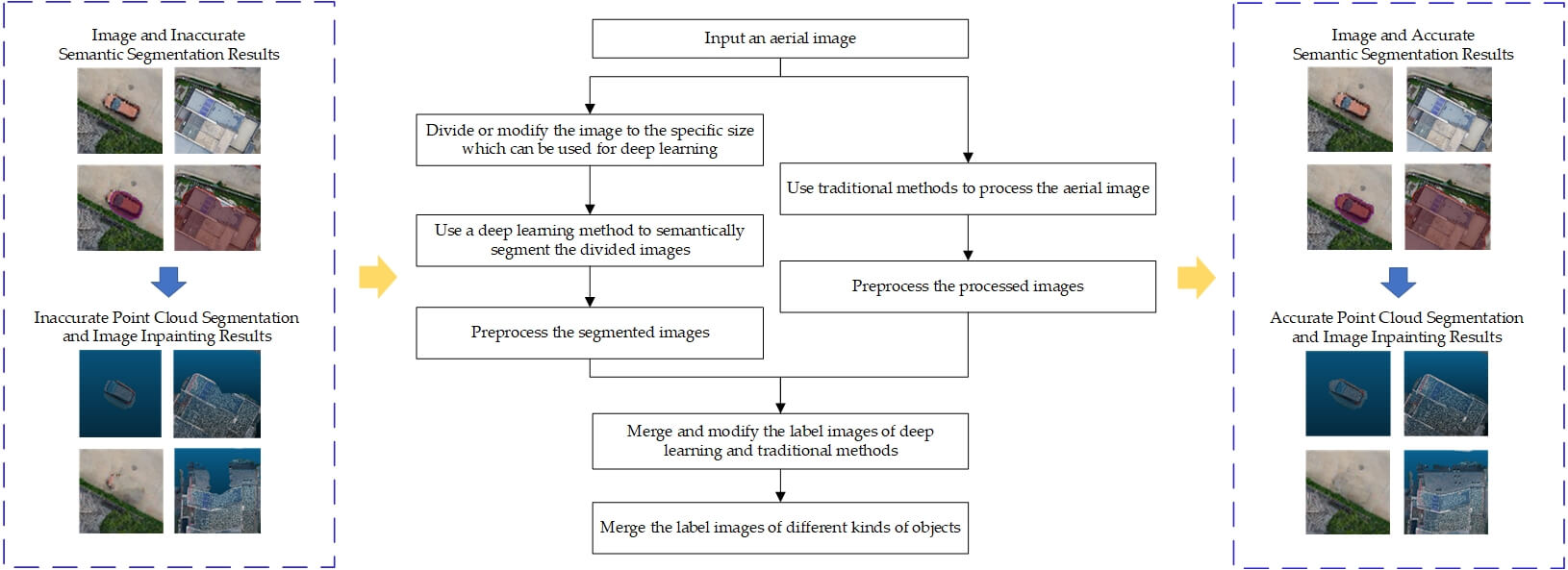
There are two types of methods for image segmentation. One is traditional image processing methods, which are sensitive to details and boundaries, yet fail to recognize semantic information. The other is deep learning methods, which can locate and identify different objects, but boundary identifications are not accurate enough. Both of them cannot generate entire segmentation information. In order to obtain accurate edge detection and semantic information, an Adaptive Boundary and Semantic Composite Segmentation method (ABSCS) is proposed. This method can precisely semantic segment individual objects in large-size aerial images with limited GPU performances. It includes adaptively dividing and modifying the aerial images with the proposed principles and methods, using the deep learning method to semantic segment and preprocess the small divided pieces, using three traditional methods to segment and preprocess original-size aerial images, adaptively selecting traditional results to modify the boundaries of individual objects in deep learning results, and combining the results of different objects. Individual object semantic segmentation experiments are conducted by using the AeroScapes dataset, and their results are analyzed qualitatively and quantitatively. The experimental results demonstrate that the proposed method can achieve more promising object boundaries than the original deep learning method. This work also demonstrates the advantages of the proposed method in applications of point cloud semantic segmentation and image inpainting.Graphic Abstract
Keywords
Image semantic segmentation is to classify each pixel in the image according to different semantic meanings and has become a leading research interest in image understanding. It plays an important role in many fields related to computer vision, such as three-dimensional (3D) reconstruction [1–3] and smart city monitoring [4,5]. In these fields, unmanned aerial vehicles (UAVs) [6,7] are usually adopted to collect aerial images because of their flexibility. Moreover, in some applications [8,9], independent detection and operation are required for individual objects that usually have obviously independent and discrete characteristics and are different from the surrounding background in aerial images. However, most remote sensing semantic segmentation methods are aimed at aerial images taken by satellites and are not applicable to UAVs [10,11]. Therefore, studying the semantic segmentation for individual objects in aerial images taken by UAVs is essential.
For example, image semantic segmentation is one of the crucial processes in 3D semantic reconstruction based on oblique photography [2,3]. In the process of reconstruction, different kinds of objects, such as buildings and cars are reconstructed separately. Specifically, by semantically segmenting top-view aerial images, a point cloud of buildings can be segmented, and buildings can be reconstructed independently. As for unnecessary vehicles during the modeling process, an image inpainting method can be adopted to remove them. However, due to high shooting height and wide scene coverage of aerial images, semantic segmentation with deep learning methods is not well handled on the edges of objects, which may lead to undesirable reconstruction results. Therefore, it is necessary to find an improved semantic segmentation method for individual objects in aerial images.
Nowadays, image segmentation methods have developed from non-semantic segmentation methods based on traditional image processing to semantic segmentation methods based on deep learning. Both kinds have their own advantages and disadvantages.
Shape, color, and texture are three prominent and common cues for recognizing objects in images [12,13], and traditional methods adopt this feature information as the basis for segmentation. These traditional methods mainly include the following: thresholding or contour-based segmentation [14,15], clustering-based segmentation [16], and graph partitioning [17,18], which respectively correspond to different feature information of images. Additionally, these methods can be used on a personal computer without a high-performance graphics processing unit (GPU) and can be used directly on large-size aerial images.
However, these methods cannot identify semantic information and may divide the objects into many small pieces. Moreover, due to the different complexity of the scene, the image feature information that plays a decisive role will be different for different images. The way to select the appropriate traditional method for image segmentation needs further research.
On the contrary, deep learning semantic segmentation methods can achieve satisfying semantic classification results on many datasets through continuous learning of semantic features and classification information. Deep learning networks, including U-Net [19–21], SegNet [22,23], PSPNet [24], DeepLab V1-V3+ [25–28], HRNet and its variants [29–32], and PFSegNets [33] are commonly adopted in semantic segmentation of datasets with large scenes and have achieved promising results in aerial image semantic segmentation.
However, constrained by GPUs and datasets, these methods are usually only applicable to images within a small size, and the results of object edges are not ideal for some applications, such as image inpainting and point cloud semantic segmentation. Therefore, deep learning methods for large-size aerial image semantic segmentation and optimizing the boundary effect of deep learning results need further research.
For large-size images, some researchers cut them into different small pieces, segment each piece by deep learning methods, and then merge them together [34,35]. However, this method requires a single target to occupy a small proportion of the image, which is unsuitable for low-altitude aerial images. Moreover, since each small piece is segmented independently, a direct combination will make mistakes at adjacent junctions. Wang et al. [36] first down-sample images and adopted a deep learning method to segment them, and then they adopted joint bilateral up-sampling to resize low-size results to original-size ones. However, this method relies on the edge shape of deep learning results and can only solve the jagging effect in the resizing process and cannot make other corrections to the boundary of objects. For the boundary effects, considering that aerial image segmentation methods usually suffer from edge information loss and poor robustness, some researchers adopt edge detection methods to guide the semantic segmentation [37] or emphasize boundaries by special structure or attention mechanism [38]. However, all of the above methods belong to modifications of the networks, which are also limited by the image size.
In the process of semantic segmentation of aerial images, the required method not only needs to be able to identify the specific semantics of different parts of the image like deep learning methods but also needs to use appropriate image feature information to obtain good boundary effects like traditional image methods without being affected by GPUs and other computing resources. Therefore, in this work, a composite semantic segmentation post-processing method for individual objects in aerial images is proposed. It is mainly applicable to individual objects in large-size aerial images taken by UAVs that need precise semantic segmentation and can be used in 3D semantic segmentation. Our main contributions include the following points:
1) An Adaptive Boundary and Semantic Composite Segmentation method (ABSCS) is proposed. It includes adaptively dividing and modifying the aerial images with the proposed principles and methods, using the deep learning method to semantic segment and preprocess the small divided pieces, using three traditional methods to segment and preprocess original-size aerial images, adaptively selecting traditional results to modify the boundaries of individual objects in deep learning results, and combining the results of different objects. It provides a new solution for the semantic segmentation of individual objects in large-size aerial images.
2) A merging and post-processing method is proposed, in which the problem of connection inconsistency and poor boundary effect in the results of the deep learning method can be modified by using the traditional results. This work also proposes a way to adaptively select the most appropriate traditional results from the results of three traditional methods according to the individual object situation.
3) Through experimental comparison on the common aerial images dataset AeroScapes, the ABSCS method shows advantages in both qualitative and quantitative results. Moreover, it can deal with some applications with specific needs. For example, completing point cloud segmentation and image inpainting when limited computing resources cannot handle deep learning models of a large size, but this size is needed to achieve a given performance.
The following part of this work is divided into the following parts: the entire process of the ABSCS method, an introduction to the choice of deep learning and traditional methods and their preprocessing, the steps of merging and post-processing deep learning results by traditional methods, as well as our experiments, applications, and conclusions.
Image semantic segmentation contains not only object recognition but also image segmentation. Deep learning methods have the advantages of object recognition, classification, and localization, while traditional methods can obtain good boundary division based on image feature information and can be directly applied to large-size aerial images. For a series of applications with high requirements for semantic segmentation of large aerial images, the advantages of both two kinds of methods are indispensable. Therefore, this work proposes an adaptive boundary and semantic composite segmentation method based on these two different mechanisms for individual objects in large-size aerial images.
2.1 Method Background and Pipeline
In this work, aerial images refer to photos taken by cameras attached to a UAV or high-altitude overhead view images similar to UAV photos, which can be used in some related applications such as 3D reconstruction. This method is applicable to both urban scene images and rural scenes, and it can process large-size aerial images with limited GPU performances and get good results. The individual objects in this work refer to objects that usually have obviously independent and discrete characteristics. These objects usually have clear boundary features or obvious color information and are different from the surrounding background. To explain and verify the method, this work adopt the common aerial images dataset AeroScapes [39], which has several individual object classes for semantic segmentation, subsequent processing, and method validation.
This work chooses one deep learning method and three traditional image processing ones as the basis of the ABSCS method. The chosen deep learning method is DeepLab V3+ [28], which has been tested on many datasets, including large street scene datasets, and has achieved good results. The chosen traditional methods are three common, basic, and typical methods, including contour finding, K-means, and grab-cut. The three traditional methods are representative of thresholding and edge-based methods, clustering-based ones, and graph partitioning-based ones, which are respectively based on shape, color, and texture feature information. These three image feature information are usually used to effectively retrieve objects in the image [12,13]. Then, the proposed ABSCS method mainly performs semantic segmentation through the following four parts.
Step 1: Dividing or modifying aerial images to the specific-size images adaptively, semantically segmenting them with a deep learning method, and preprocessing the results to obtain multiple labels with only one kind of objects in each label.
Step 2: Segmenting original-size aerial images with different traditional processing methods and preprocessing the results to obtain multiple traditional labels including only one kind of traditional information in each label.
Step 3: Selecting an appropriate traditional label in Step 2 for each deep learning label in Step 1. Then, merging and modifying the labels to get the final result of each kind of objects.
Step 4: Combining the final results of different kinds of objects into a unified label.
The whole pipeline of the ABSCS method is shown as Fig. 1.

Figure 1: The whole pipeline of the ABSCS method
Considering that our method is suitable for individual objects in aerial images, this work adopts the common aerial images dataset AeroScapes [39] to explain and verify the composite method. AeroScapes is a collection of 3269 aerial images from 141 video sequences and their associated semantic segmentation labels. The images are captured by a fleet of UAVs operating at an altitude of 5 to 50 m, and their size is 1280 × 720.
In AeroScapes, the labels are labeled with both stuff classes such as vegetation and roads and thing classes such as people and cars. In this work, individual objects mainly refer to the thing classes. However, the class distribution in AeroScapes is imbalanced, and the cumulative weights of some things are very low. Therefore, to ensure adequate training and validation data, this work only chooses the top four high-weight thing classes as the basis of our quantitative analysis–obstacle, person, car, and animal. Some aerial images and their semantic segmentation labels of AeroScapes are shown in Fig. 2.

Figure 2: Examlples of AeroScapes: (a) aerial images and (b) segmentation labels
2.3 Deep Learning Image Semantic Segmentation
Deep learning semantic segmentation is one of the basic elements of our method. It mainly provides semantic information and locations of objects, which is convenient to be combined with the results of traditional methods for subsequent post-processing and optimization.
Considering the advantages and disadvantages of deep learning methods and the actual applications, the main work in this part is as follows. First, the appropriate deep-learning method is chosen for UAV aerial images covering street scenes. Second, in order to process large-size images with limited GPU performances, the aerial images are divided or modified by the proposed principles with maximum utility according to the characteristics of the deep learning method. Finally, the deep learning method is adopted to semantically segment small-size images, and a preprocessing method is proposed for the segmented results to make them suitable for subsequent merging steps.
Considering that the post-processing method in this work is processed on the basis of deep learning results, the accuracy of deep learning results directly influences the final accuracy. A good deep-learning network can provide accurate semantic recognition and good preliminary boundary segmentation. Many semantic segmentation deep learning networks that are suitable for large street scene aerial images can be used in this section. By comparing the results of different networks on large scene datasets, in order to achieve good final experimental results, DeepLab V3+ [28] is chosen to segment the images.
DeepLab V3+ is an improved version of DeepLab V3 [27]. DeepLab V3+ combines the spatial pyramid pooling module and the encode-decoder structure, which not only can encode multi-scale contextual information but also can recover spatial information gradually. It adopts DeepLab V3 as the encoder to design a simple and efficient decoder. It also adopts Xception [40] model and applies the depthwise separable convolution to Atrous Spatial Pyramid Pooling (ASPP) and decoder. Then, a strong encoder-decoder structure can be constructed. By using DeepLab V3+, different kinds of objects are semantically segmented in different colors. Thus the boundaries and the categories of objects can be distinguished by label colors.
In DeepLab V3+, Chen et al. used two kinds of network backbone, Xception and ResNet-101, to compare the model variants in terms of both accuracy and speed [28]. Moreover, different backbone models can be chosen for DeepLab V3+. For example, Deep Residual Network (DRN) model [41] can be the backbone network as well. Zhang et al. [42] adopted four neural network architectures (U-net, DeepLab V3+ with ResNet, DRN, and MobileNet as the backbones) to identify glaciological features such as calving fronts from multi-sensor remote sensing images, and the result using DRN-DeepLab V3+ achieves the lowest test error. The advantage of DRN is that it can keep the receptive field of the original network without losing the resolution of images. For aerial images, some individual objects usually occupy only small areas in the whole image scene. If the image size is reduced further, these objects will probably resize to a single pixel or even disappear, which may lead to missing details. Therefore, it is very important to keep enough image size for semantic segmentation of individual objects. From the perspective of semantic segmentation accuracy and visual effects, this work chooses DeepLab V3+ network with DRN as the backbone model to semantic segment the images.
2.3.2 Aerial Image Adaptive Division and Modification
Some aerial images captured by UAVs usually have large image sizes. However, limited by computing resources such as GPUs and the design of the network, one deep learning method can only deal with images with one specific small image size, and both large-size and small-size images need to be adjusted to this specific size at first. In order to avoid the reduction of detailed information, this work chooses to divide the large-size images into small pieces instead of down-sampling the images. Combined with the situation of DeepLab V3+, the input images are processed to the size of 512 × 512. Considering that the size of aerial images from different sources is different, methods with strong applicability are needed for image division and modification. Therefore, an adaptive division and modification method is proposed in this work.
The first principle of division is to ensure that the objects are not distorted, such as being stretched or widened. The second principle of division is to keep the size of objects as constant as possible. The third principle of division is that there should be as few small-size images as possible to save the time of deep learning semantic segmentation. Therefore, for the aerial image with a size lower than 512 × 512 and that with a size higher but close to 512 × 512, the image is cut into a square according to its short edge and then resized to 512 × 512. For the aerial image with a size much higher than 512 × 512, there are two kinds of division methods used in this work. The first method is to cut the aerial image from the top left corner until the 512 × 512 image can no longer be cut. The large image is divided into non-overlapping small images, and the right edge pixels are discarded. If the image resolution is m×n, then the number i of small images can be calculated as follows:
The second method is to ensure all pixels in large images are cut into small ones. This method makes the image overlap when the image resolution is not divisible by 512. The number i of small images is
When m/512 are not integers, the number of overlapping pixels is
When n/512 are not integers, the number of overlapping pixels is
An example of division is shown as Fig. 3, where a large image with the size of 4439 × 5137 [43] is divided by both the first and the second methods. Fig. 3a shows the original large-size image. In Fig. 3b, 8 × 10 pieces of images with the size of 512 × 512 are obtained. In Fig. 3c, 9 × 11 pieces of images with the size of 512 × 512 are obtained.

Figure 3: Division of a large-size image. (a) Image; (b) First method result; (c) Second method result
2.3.3 Segmentation and Preprocessing of Small Images
The semantic segmentation of a specific size image is carried out by using the selected DeepLab V3+ network with DRN. After that, a preliminary segmentation label can be obtained, and each pixel color of the label represents one kind of object. For example, blue represents cars and green represents people. Meanwhile, the label image needs to be further processed to make it more suitable for the subsequent label merging. The preprocessing of deep learning results is mainly divided into the following three steps.
Step 1: To process different kinds of objects individually, this work separates the objects in the label image according to their label color. For example, if there are both cars and people in a label image, the cars and people can be separated into two different labels according to the colors. Each label is a black and white one, in which white is the foreground and black is the background.
Step 2: To facilitate subsequent merging, this work modifies the foreground label pixel value to α for each label image, in which α is a constant less than 255. For illustration purposes, α is set to 60 here. Then new label images are obtained.
Step 3: To prepare for selecting the most appropriate traditional method for each label area in the label image, this work counts and records the connected components in the label image with the seed fill algorithm. In the seed fill algorithm, label areas with different pixel values represent different connected components for intuitive display.
2.3.4 Example of Deep Learning Image Semantic Segmentation
In this paper, an image is taken as an example. This is an image with people and cars, and its size is 1280 × 720 [39], which is higher but close to 512 × 512. Therefore, the image is cut into a square according to its short edge and is resized to 512 × 512. Then, the deep learning semantic segmentation and preprocessing are performed according to Section 2.3.3. The result is shown in Fig. 4.

Figure 4: Schematic diagram of Section 2.3
2.4 Traditional Image Segmentation
The principles of traditional image segmentation methods are varied. They mainly provide segmentation based on image feature information, and their results are consistent with visual perception. Moreover, they can directly process large-size images without the limitation of GPUs, so there is no problem of incoherent boundaries caused by image cutting and splicing. Therefore, before optimizing the object boundaries obtained by deep learning, the traditional image segmentation results need to be obtained and preprocessed.
The main work in this part is as follows. First, the appropriate traditional methods according to the actual demand are analyzed. This work mainly adopts three traditional image processing methods, including contour finding, K-means, and grab-cut, from which this work can obtain different typical features of images. Then, different traditional methods are adopted to process aerial images, and a preprocessing method for the traditional results is proposed to make them suitable for subsequent merging steps.
2.4.1 Traditional Segmentation Methods
Thresholding and edge-based methods, clustering-based ones, and region-based ones are three kinds of common, basic, and typical traditional image segmentation methods, and there are many other methods similar to them and based on their improvements. They are respectively based on shape, color, and texture feature information, which are usually used in image retrieval. Among them, thresholding and edge-based methods adopt the gradient of image pixels and regard the gradient reaching a certain threshold as a boundary. Clustering-based methods adopt distances between pixels or pixel color similarity to segment images and can group the pixels with similar properties. Region-based methods treat image segmentation as a graph partitioning problem, and they adopt graph theory to segment the images from a geometric perspective.
Considering that aerial images cover a wide range of scenes and the individual objects have different characteristics, to make the results of the traditional methods as general as possible, this work chooses three methods on behalf of thresholding and edge-based methods, clustering-based ones, and region-based ones, and adopts an adaptive one to carry out label merging and modification in the subsequent merging steps. The chosen three methods are contour finding, K-means, and grab-cut, in which contour finding can provide contours of objects, K-means can provide color-clustering groups, and grab-cut can provide foreground things. The above three kinds of information not only represent most of the obvious categories of object features but also correspond to human visual perception.
The contour finding method adopts the changes of pixel values between two different objects to achieve segmentation, which is suitable for individual object extraction. It can outline the boundary of the objects. The boundary is a closed curve, so the inner and outer parts of the curve can be distinguished. Usually, the inner and outer parts represent different things.
The K-means method is a clustering-based unsupervised segmentation method, and it is sensitive to colors. Its basic steps are as follows. First, the number of clusters needs to be given according to the requirement and set k centroids in random places. Then, each point is assigned to the nearest centroid, and the centroid is moved to the center of a new cluster after that. Finally, the previous process is repeated until the stop criterion is reached. However, objects in aerial images are usually not simple solid color objects. When the value of k is large, the image will be divided into too many parts, and some aerial images with noise may cause dense miscellaneous points after segmentation. When the value of k is small, the segmentation boundary of different objects will be unclear, which will affect our subsequent steps. After experimental comparison and considering three primary colors, k is set to 3 in this work.
The grab-cut method is an iterative interaction method based on graph theory and adopts texture and boundary information in the images. The iteration times and the approximate position of the objects (the bounding box of the objects) need to be set before processing the images. The pixels in the bounding box contain the main object and the background. The circumscribed rectangles of the connected components obtained by the preliminary deep learning semantic segmentation results can be used as the bounding boxes, and an appropriate number of iterations can be set to 20. This work iterates the segmentation on different connected components that are recorded in the Step 3 of Section 2.3.3 and gets the grab-cut results of each connected component after iterative graph partition.
In the example of Section 2.3.4, there are two connected components of cars and two connected components of people in the image. Since te grab-cut method needs to be given a bounding box, the connected component of one car is taken as an example to explain the procedure. This work adopts the contour finding method to find the edges of the object, the K-means method to perform color clustering, and the grab-cut method to perform a segmentation result with one bounding box. Fig. 5 shows the visual effects of different traditional methods.

Figure 5: Car result of different traditional methods
2.4.2 Segmentation and Preprocessing Based on Traditional Results
As shown in Fig. 5, after using traditional methods, the preliminary results that show boundary information, color information, and foreground information can be obtained. However, these images are not labeled images and need to be further processed to make them suitable for subsequent label merging steps. This work adopts different preprocessing methods for each traditional result because the output results of different traditional methods vary a lot.
The result of contour finding needs the following preprocess:
Step 1: Calculate the length of each contour in the image and delete some very short ones.
Step 2: Fill the inside of the new contour image to make white inside the contour and make black outside the contour. Then, fill the outside of the new contour image to make white outside the contour and make black inside the contour.
Step 3: Modify the white pixel value to β for each image obtained by Step 2, in which β is a constant less than 255, and α in Section 2.3.3 plus β should be less than or equal to 255. For illustration purposes, β is set to 120 here. Then, new label images are obtained.
Step 4: Count and record the connected components in the label images with the seed fill algorithm, resulting in label areas with different pixel values representing different connected components for intuitive display.
Fig. 6 shows the results of the steps with the above-mentioned contour method.

Figure 6: Segmentation and preprocessing based on contour result
The result of K-means needs the following preprocess:
Step 1: Separate different colors’ labels, make the foreground white and make the background black in each new label. Then, three images with objects containing different colors are obtained.
Step 2: Modify the white pixel value to β for each image obtained by Step 1, in which β is a constant less than 255, and α in Section 2.3.3 plus β should be less than or equal to 255. For illustration purposes, β is set to 120 here. Then, new label images are obtained.
Step 3: Count and record the connected components in the label images with the seed fill algorithm, resulting in label areas with different pixel values representing different connected components for intuitive display.
Fig. 7 shows the results of the steps using above-mentioned K-means.

Figure 7: Segmentation and preprocessing based on K-means result
The result of grab-cut needs the following preprocess:
Step 1: Take the pixels that are not black as the foreground, make the foreground white and make the background black in the label.
Step 2: Modify the white pixel value to β for each image obtained by Step 1, in which β is a constant less than 255, and α in Section 2.3.3 plus β should be less than or equal to 255. For illustration purposes, β is set to 120 here. Then, new label images are obtained.
Step 3: Count and record the connected components in the label images with the seed fill algorithm, resulting in label areas with different pixel values representing different connected components for intuitive display.
Fig. 8 shows the results of the steps using the above-mentioned grab-cut.

Figure 8: Segmentation and preprocessing based on grab-cut result
2.5 Label Merging and Modification
For different individual objects, in order to carry out label modification and boundary optimization in combination with their own characteristics, an adaptive method for selecting appropriate traditional labels to merge with deep learning labels is proposed. By finally merging different individuals and different kinds of objects, a modified image label is obtained, which not only has clear and coherent boundaries but also contains semantic information about the object. The whole process of the merging algorithm is introduced here.
2.5.1 Adaptive Selection of Traditional Labels
Different objects have different characteristics. For example, the independent characteristic of cars is obvious, and the color characteristic of trees is obvious. Moreover, for different individual objects of the same class, differences also exist due to their colors and structures. The connected components are the basis for distinguishing between individual objects of the same class. Therefore, this work proposes an adaptive selection of traditional labels to merge and modify each connected component in each deep learning label.
According to the segmentation and preprocessing of the above-mentioned traditional methods, for each connected component in the deep learning label, two corresponding contour labels, three corresponding K-means ones, and one corresponding grab-cut one can be obtained. The adaptive selection consists of two parts. In the first part, the most appropriate contour label and the most appropriate K-means one are selected respectively for each connected component in the deep learning label. In the second part, the most appropriate traditional label is selected from the above contour label, the above K-means one, and the grab-cut one.
To be specific, in the first step, two contour labels and three K-means labels are added to the deep learning label, respectively, to obtain the merged labels. Each pixel value in each merged label can be computed as:
where i and j represent the x-coordinate and the y-coordinate of each pixel in the image, DVij is the value of (i, j) pixel in the deep learning label, TVij is the value of (i, j) pixel in the traditional label, DTVij is the value of (i, j) pixel in the merged label. In this way, the preliminary five merged labels can be obtained. On each merged label, there are four kinds of pixel values (0, α, β, α + β), in which α and β are the deep learning label value and the traditional label value mentioned in Sections 2.3.3 and 2.4.2, respectively. Therefore, the pixel value of 0 indicates the background, the pixel value of α + β indicates the common objects, and the pixel value of α or β indicates that further determination is needed. Then, the numbers of pixels valued α + β in the merged labels are counted, respectively. The merged label with the largest number is the most appropriate label. Thus, the most appropriate contour and K-means labels are obtained.
In the second step, similarly, the grab-cut label is added to the deep learning one, and the number of pixels valued α + β is counted in the merged one. After comparing the numbers of pixels valued α + β in the merged labels obtained by the grab-cut label, the above contour label, and the above K-means label, the merged label with the largest number is considered to be the most appropriate traditional label.
For the car example in Fig. 5, the most appropriate labels of different methods and their merged labels are shown in Fig. 9.

Figure 9: The most appropriate labels of different methods and their merged labels: (a) the contour label, (b) the K-means label, (c) the grab-cut label, (d) the traditional label, (e) the contour merged label, (f) the K-means merged label, (g) the grab-cut merged label, and (h) the traditional merged label
2.5.2 Merging of Traditional and Deep Learning Labels
In Section 2.5.1, by superimposing traditional labels and deep learning ones, four preliminary most appropriate merged labels are obtained for each deep learning connected component. In this section, this work proposes a merging method to further select and process these preliminary merged labels to obtain the final label. The merging method includes three steps.
Step 1: If the traditional label is similar enough to the deep learning one, retain the traditional label.
In Sections 2.4.2 and 2.4.3, the connected components in the traditional labels of contour, K-means, and grab-cut are counted and recorded. To judge whether each connected component in traditional labels is similar enough to the objects in the deep learning label, this work takes the connected components in the traditional label as the bases and adopts the traditional label-based overlap ratio (TOR) of each connected component as the indicator, and the indicator value VTOR is calculated by the following equation:
where CNT is the number of pixels valued β in this region of the traditional label, CNDT is the number of pixels valued α + β in the same region of the merged one. Higher VTOR means higher similarity of the connected component between two labels.
A threshold TTOR is set for VTOR, which ranges from 0 to 1 and can be changed according to different situations. When VTOR < TTOR, it is considered that there is something else in this connected component of the traditional label, and nothing should be done about this region. Otherwise, it is considered that this connected component in the traditional label is sufficiently similar to the same region in the deep learning label, and the same pixels in the most appropriate traditional merged label are adjusted to α + β.
Therefore, in practice, the operations of Step 1 are as follows. Firstly, this work calculates the VTOR of each connected component in the most appropriate contour label and retains the component whose VTOR >= TTOR. For those connected components whose VTOR >= TTOR, this work calculates the total number of pixels whose value is α + β in the same region of the merged label. Secondly, this work conducts the same operation for the most appropriate K-means and the grab-cut labels. Thirdly, by comparing the total number of pixels in three merged labels, the traditional label whose total number is the largest can be obtained, which is considered to be the most similar label to the deep learning label and can be used to modify the merged label. Finally, for the most similar traditional label, if VTOR >= TTOR, this work changes the pixels in the same region of the most appropriate traditional merged label to the value of α + β.
In the example, the VTORs of both two cars in the image are higher than TTOR, so the traditional label parts are directly put into the merged label. After this step, the most appropriate traditional merged labels of the two cars are shown in Fig. 10.

Figure 10: The most appropriate traditional merged labels after Step 1: (a) the first car, (b) the second car
Step 2: If there is a big gap between the deep learning label and the traditional one, retain the deep learning label.
This work takes the connected components in the deep learning label as the bases to judge whether the objects are not well detected by the most appropriate traditional merged label that has been already modified by Step 1. The deep learning label-based overlap ratio (DOR) is adopted as the indicator, and the indicator value VDOR is calculated by the following equation:
where CND is the number of pixels valued α in this connected component of the deep learning label, and CNDT is the number of pixels valued α + β in the same region of the modified most appropriate merged label.
This work separates each connected component in its deep learning label and calculates the VDOR value of each connected component. A threshold TDOR is set for VDOR. TDOR ranges from 0 to 1 and can be changed according to different situations. If VDOR >= TDOR, it is considered that the big gap between the two labels does not exist, and nothing should be done about this region. Otherwise, it is considered that this region is not well detected by the most appropriate traditional label. Therefore, the original region in the deep learning label is regarded as the final result directly, and the pixels in the same region of the most appropriate traditional merged label are adjusted to the value of α + β.
As shown in Fig. 11a, VDOR of the first car is lower than TDOR, and therefore, the deep learning label part is directly put into the merged one. However, as shown in Fig. 11b, VDOR of the second car is higher than TDOR, and therefore, nothing should be done about the merged label.

Figure 11: The most appropriate traditional merged labels after step 2: (a) the first car, (b) the second car
Step 3: Fill in the missing parts of the merged label.
To avoid small parts of objects being detected by the deep learning method but not detected by traditional methods, the missing parts should be further filled in the modified most appropriate merged label. As shown in Fig. 12, the regions in the red boxes are the regions that need to be filled for the second car.

Figure 12: Schematic diagram of label filling regions
The filling parts mainly consider the following situations:
1) The region exists continuously in the deep learning label but not in the traditional label;
2) The region with a large boundary gap between the merged label and the deep learning label;
3) The large region is present in the deep learning label but not in the merged label.
The judgment and the corresponding filling methods of different situations are introduced in detail.
• Situation 1
Situation 1 refers to the regions whose pixel values are not α + β in the most appropriate traditional merged label, but the regions themselves and their surrounding pixels are all valued α in the deep learning label. For this kind of regions, their pixels in the modified most appropriate traditional merged label are adjusted to the value of α + β.
• Situation 2
For situation 2, the most modified appropriate traditional merged label is detected and processed.
Firstly, a small square (this work takes a small square with a side length of 1/50 of the original image side length) is looped along the boundaries of the regions where their pixel valued α + β. If there is no background (pixel valued 0) in this square, this square is considered to be a missing region, and the value of the pixels in this square is set to α + β. Secondly, the square is looped along the boundaries of the newly added α + β regions until no newer α + β regions appear. Thirdly, the side length of the square is gradually reduced, which depends on the following equation:
The side length of the square is reduced by half, and the new square is continued to loop along the boundaries of newly added α + β regions found in the above steps. This work loops through the above process and reduces the side length of the square until its side length is one pixel.
After the end of the loop, in the newest merged label, it is judged whether the surrounding pixel values of each connected component whose pixel value is α are all 0 or newly added α + β. If its surrounding pixel values are all 0 or newly added α + β, the pixel values of this connected component are adjusted to α + β.
The flow chart is shown in Fig. 13.

Figure 13: The flow chart of situation 2
• Situation 3
The pixels whose values are α are marked in the merged label processed after situation 2. A small square (this work takes a small square with a side length of 1/50 of the original image side length) is looped along the marked pixels. If the square is full of marked pixels, this central pixel is considered to be a missing one and the pixel value is set to α + β. After the end of the loop, in the modified merged label, it is judged whether the surrounding pixel values of each connected component whose pixel value is α are all 0 or newly added α + β. If its surrounding pixel values are all 0 or newly added α + β, the pixel values of this connected component are adjusted to α + β.
The modified merged result for the second car is shown as Fig. 14. In Fig. 14, the pixel valued α + β means the label result of the second car after the filling method, and the pixel valued α means the discarded deep learning result.

Figure 14: The modified merged result for the second car
2.5.3 Combination of Same Objects
In Sections 2.5.1 and 2.5.2, this work finds the corresponding appropriate traditional label for each connected component in each deep learning label and merges the traditional label and the deep learning label. Considering that the same kind of objects end up with the same color in the final label, for the modified merged label corresponding to each connected component in one deep learning label, it is necessary to set the pixel values at the same position on the final label of this category to 255 and other pixel values to 0. The final label for cars is shown as Fig. 15.
Figure 15: The final label for cars
2.6 Combination of Different Objects
When labels of different kinds of objects are combined and label pixels are overlapped, it is necessary to set priorities for labels of different kinds of objects and make the final semantic segmentation label according to the priorities. The label with high priority is the category in which the overlapping pixels are classified. For example, if a person is holding a dog and the modified person label overlaps the modified dog one. And if the person label has high priority, the final label of the overlapping pixels is the person instead of the dog. To reasonably determine priorities, this work considers the object labels that are similar to the ground truth results to be given high priority. Since the ground truth in practical applications cannot be known, the result of deep learning is used as a substitute.
In Section 2.5.2, this work takes the connected components in the deep learning label of one kind of objects as the bases and calculates the indicator value VDOR of each connected component. Therefore, for each kind of objects, the average VDOR of different connected components can be calculated. High VDOR means that the big gap between the deep learning label and the original most appropriate traditional one does not exist. Therefore, objects with a high value of average VDOR have a high priority. Finally, the results of different objects can be merged according to their priorities, and the colors are adjusted to the original colors in the deep learning label.
The deep learning results and the final results for the image are shown in Fig. 16, in which the blue labels mean cars and the green labels mean people. It can be seen that the final result is more detailed and overlaps more with the original image than the deep learning result.

Figure 16: The deep learning results and the final results for the image: (a) the deep learning label, (b) the deep learning visualization results, (c) the final label, and (d) the final visualization results
To verify the effectiveness of the ABSCS method, this work conducts qualitative and quantitative experiments in this section on a PC with an NVIDIA GTX 1080 Ti GPU. Constrained by the GPU, the input images of the deep learning method are processed to the size of 512 × 512. In combination with the AeroScapes dataset, two metrics are selected for subsequent quantitative analysis. As for qualitative and quantitative experiments, this work first adopts aerial image examples to make qualitative analysis according to the steps in Section 2. Then, the selected metrics are adopted to carry out the statistical calculation on the datasets for quantitative analysis. Finally, to verify the effectiveness of the ABSCS method in the application of 3D semantic reconstruction, the effects on 3D point cloud segmentation and image inpainting are tested.
This work adopts two metrics to assess labeling performance. The first metric is a global performance one that is commonly known as the intersection-over-union metric (IoU) [44]. IoU value VIoU can be calculated as the following equation:
where TP is the number of true positive pixels, FP is the number of false positive pixels, and FN is the number of false negative pixels. VIoU of each kind of objects represents the global accuracy of semantic segmentation, and it is determined over the whole test dataset. VIoU is distributed in the range of 0 ∼ 100%. High VIoU means a good segmentation effect.
The second metric describes the edge performance, which is a measure of pixel distance named median absolute deviation (MAD) [45]. The set of boundary points of the result obtained by our segmentation method is set as B = {bi: i = 1, …, K} (K is the total number of boundary points), the set of boundary points of the original ground truth result is set as T = {tn: n = 1, …, N} (N is the total number of boundary points), and the distance from the point to the boundary is set as d (B, tn) = min |bi – tn|. Based on the original ground truth result, MAD value VMAD is calculated as the following equation:
MAD represents the pixel difference of the segmentation boundaries before and after merging. VMAD of each kind of objects represents the edge accuracy of semantic segmentation, and it is determined over the whole test dataset. Low VMAD means close boundaries and a good segmentation effect.
To qualitatively and quantitatively analyze the ABSCS method, this work carries out experiments on the AeroScapes images. In Section 2, two thresholds TTOR and TDOR need to be set before experiments. After an experimental comparison of visual and data effects of different values of TTOR and TDOR, the TTOR value is set to 0.85 and the TDOR value is set to 0.8.
This work selects one image for each class chosen in Section 2.2, including obstacle, person, car, and animal. Qualitative results are shown in Fig. 17. For each image, the standard label, the deep learning one, the most appropriate traditional one and the final one are shown.

Figure 17: Visual results of different kinds of objects in AeroScapes: (a) standard label of obstacle, (b) deep leaning label of obstacle, (c) most appropriate traditional label of obstacle, (d) final label of obstacle, (e) standard label of person, (f) deep leaning label of person, (g) most appropriate traditional label of person, (h) final label of person, (i) standard label of car, (j) deep leaning label of car, (k) most appropriate traditional label of car, (l) final label of car, (m) standard label of animal, (n) deep leaning label of animal, (o) most appropriate traditional label of animal, and (p) final label of animal
From the above experimental results, it can be seen that the deep learning method can obtain true semantic information in the images. Although the most appropriate traditional labels are also selected based on the deep learning labels, the traditional labels are not semantic and also have some other wrong identifications. For example, the missing part in the center of the obstacle and the animal, and the extra part of the stair beside the person. On the contrary, in terms of boundary effect, the results of the most appropriate traditional labels are better than those of the deep learning labels. This is also related to the working principle of the traditional processing methods, which is based on the feature information of the images. Since the proposed method adopts the traditional labels to carry out post-processing on the deep learning labels, the final result has a high similarity with the deep learning result. This feature is reflected in both qualitative and quantitative analysis. However, it is observed that the final labels after post-processing are modified by the traditional labels and are closer to the real boundaries of objects than the deep learning labels. These include the upper part of the sign, the cyclist’s arm, the front and rear edges of the car and its rearview mirrors, and the back of the panda. For some objects with obvious individual characteristics, our method can obviously solve the problems that the boundary locations are not ideal and the boundary edges are smooth in deep learning results. Qualitative experiment results show that the ABSCS method is helpful in optimizing the semantic segmentation results of individual objects in aerial images.
This work conducts deep learning and post-processing experiments for the four kinds of objects in the test sets of the AeroScapes dataset. Considering that the final results are based on deep learning results and only when they are well identified that our method can well modify the results, this work especially calculates VIoU and VMAD for the well-identified objects whose VIoU is over 60%. In order to demonstrate the advances of the proposed method, this work also compares the ABSCS results with the results of the HRNet [29,30] + OCR [46] method and the PFSegNets [33] method. The HRNet + OCR method is widely recognized in the field of high-resolution image semantic segmentation, and the PFSegNets method is a state-of-the-art one that is specially designed for aerial image segmentation. Their quantitative results are shown in Tables 1 and 2, which show VIoU and VMAD of different kinds of well-identified objects.
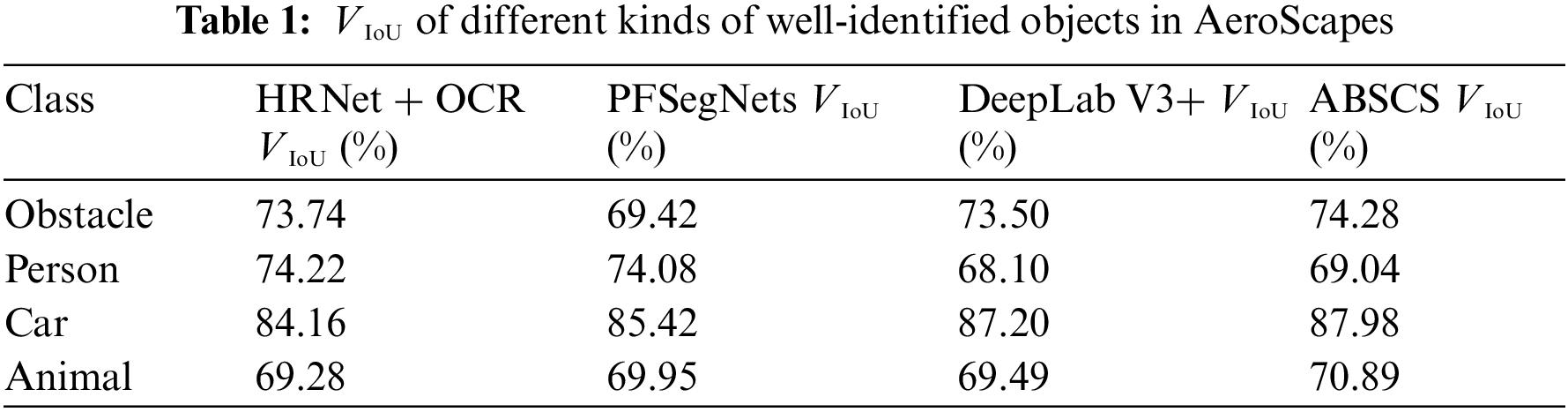

High VIoU and low VMAD indicate the high accuracy of the results. As shown in the above experiments, in terms of VIoU, the ABSCS method gets better performance in obstacle, car, and animal than the deep learning methods. The PFSegNets method and the HRNet + OCR method get the top two performances in person. However, as for VMAD, the ABSCS method achieves the best result in person and the second best results in obstacle and car. The PFSegNets method and the HRNet + OCR method achieve the best result in obstacle and car, respectively. Although the ABSCS method has a much higher VMAD in animal, this is also related to the relatively small number of images containing animals resulting in a great contingency. Therefore, the overall effect of the ABSCS method is better than that of the deep learning methods.
Moreover, to further illustrate the improvement of the composite method on the used DeepLab V3+ method, this work also calculates the absolute and relative growths of VIoU and VMAD. The results are shown in Table 3.

Since the proposed ABSCS method is the post-processing of deep learning results and mainly improves the boundaries of objects, VIoU of the ABSCS method achieves an improvement of about 1%. However, the absolute and relative growths of VMAD show that the ABSCS method has made relatively great progress in boundary optimization. Quantitative results show that the ABSCS method is helpful in optimizing the semantic segmentation results of individual objects in aerial images.
From the perspective of engineering practices, a small deviation in a boundary can make a big difference. In this work, the effectiveness of the ABSCS method is verified in 3D semantic reconstruction, including the applications of point cloud semantic segmentation and image inpainting.
The proposed ABSCS method can be used to deal with the semantic segmentation of large-size images. As shown in Fig. 18, when an aerial image with the size of 1024 × 1024 is taken from a low-view point, a building may occupy a large area of the image, while a car may occupy a small area. Due to the limitation of GPUs, deep learning methods may can not directly process a large-size image. If the image is down-sampled to the size of 512 × 512, the deep learning semantic segmentation method may get unsatisfied results, and if the image is cut into four pieces, unnecessary trouble may occur at adjacent junctions.

Figure 18: Large-size image and its semantic segmentation results with different methods: (a) the large-size image with building and car examples, (b) the down-sampled semantic result with building and car examples, and (c) the cut and merged semantic result with building and car examples
For example, in Fig. 18a, it can be seen that the large building in the red box is in the center of the image, while the small car in the yellow box is in the lower-left corner of the image. Different methods are adopted to semantically segment the image, and in deep learning results, buildings are red and cars are purple. In Fig. 18b, the image is down-sampled to 512 × 512, and DeepLab V3+ is adopted to semantically segment the down-sampled image. It is shown that the result after down-sampling is not ideal, many objects are connected together and the boundary effect is very poor. Some small objects, such as cars, cannot even be detected. In Fig. 18c, the image is cut into four 512 × 512 pieces, and the DeepLab V3+ method is adopted to semantically segment the pieces, and then the results are stitched to the original size. It is shown that the boundary effect of objects is good. Yet, for the building in the center, there is a clear patchwork of pieces in the up part of the building. To achieve good application effects, this work adopts Fig. 18c for the next validation.
In 3D semantic reconstruction, different operations need to be performed on different objects according to actual requirements. For example, when only immovable objects are important, buildings need to be modeled and cars need to be removed, but when all objects are important, both buildings and cars need to be modeled separately. To illustrate the effectiveness of the proposed method, this work takes the car in the yellow box and the building in the red box in Fig. 18 as examples, and adopts the deep learning results and the final results with the ABSCS method to conduct comparative experiments. In view of the above two applications, this work carries out image inpainting and point cloud semantic segmentation for the car and point cloud semantic segmentation for the building. The segmentation and application results are shown in Fig. 19. From Fig. 19, it is shown that the label boundaries of both the car and the building are improved, which directly improves the effects of the subsequent application of image inpainting and point cloud semantic segmentation.

Figure 19: Segmentation and application results: (a) original car image, (b) complete car point cloud, (c) original building image, (d) complete building point cloud, (e) deep learning car label, (f) final car label, (g) deep learning building label, (h) final building label, (i) point cloud segmentation based on deep learning car label, (j) point cloud segmentation based on final car label, (k) top view of point cloud segmentation based on deep learning building label, (l) top view of point cloud segmentation based on final building label, (m) image inpainting based on deep learning car label, (n) image inpainting based on final car label, (o) side view of point cloud segmentation based on deep learning building label, and (p) side view of point cloud segmentation based on final building label
For the car, Figs. 19e and 19f show that the front of the car is well modified. In Fig. 19m, the texture of the car cannot be completely eliminated and will affect the texture of the road, yet this situation has been resolved in Fig. 19n. For the complete car point cloud in Fig. 19b, when semantic segmentation results are adopted to segment the car point cloud, compared with Figs. 19i and 19j can separate the car more completely, and therefore, more points of the car can be used for subsequent applications.
For the building, from Fig. 18c, it can be seen that at the joint of four pieces, which is also in the middle of the building in Fig. 19g, there is a horizontal line with obvious splicing. Through the modification using the proposed ABSCS method, the final building label in Fig. 19h is close to the real situation. Moreover, when 3D semantic reconstruction is carried out, buildings often need to be detected separately, and therefore, the building point cloud can be adopted to further carry out 3D mesh reconstruction and texture mapping. Figs. 19k and 19o show that the segmented building point cloud using the deep learning label have a huge gap. By using the modified building label, Figs. 19l and 19p segment the building point cloud completely, and the points in the gap are well-identified.
It is worth mentioning that the ABSCS method has relatively large modification potential, which is mainly reflected in the following three aspects:
• Replaceability
The ABSCS method is based on traditional image processing and deep learning processing methods. In this work, only three typical traditional methods and one suitable deep learning method are adopted to illustrate the validity of the composite method. However, the traditional methods and the deep learning method can be replaced by other state-of-the-art methods. Especially, deep learning methods are constantly updated nowadays, and if there is a more suitable deep learning semantic segmentation method for aerial images in the future, the current method can be further replaced.
• Practicability
The ABSCS method is not only applicable to aerial images but also applicable to other daily ones, such as street view ones and indoor ones. For different scenarios and user needs, thresholds can be modified to yield ideal results.
• Generalizability
Many steps are based on connected components, and the current method can be applied to other fields such as instance segmentation in the future. Meanwhile, the ABSCS method can be further improved to deal with many other real-life applications such as object grab and autopilot.
This work proposes an Adaptive Boundary and Semantic Composite Segmentation (ABSCS) method for individual objects of aerial images, which can process large-size images with limited GPU performances. By adaptively dividing and modifying the aerial images with the proposed principles and methods, using the deep learning method to semantic segment and preprocess the small divided pieces, using three traditional methods to segment and preprocess original-size aerial images, adaptively selecting traditional results to modify the boundaries of individual objects in deep learning results, and combining the results of different objects, this work can not only identify the semantic information but also give the explicit object boundary information. Qualitative experiments demonstrate that compared with the deep learning results, the ABSCS results are more consistent with the boundary of the objects in terms of visual perception. The results are also improved in the quantitative experiments in terms of the global intersection-over-union metric and the median absolute deviation metric. Finally, the validity and necessity of the ABSCS method are discussed through experiments on applications of image inpainting and point cloud semantic segmentation.
The ABSCS method has the advantages of replaceability, practicability, and generalizability. It can be replaced later when new deep learning or traditional methods become available, can be modified and applied to other images of different fields, and can be extended to instance segmentation or other image semantic segmentation. In addition, the use of multiple views or videos may also improve segmentation effects [47]. After the improved semantic segmentation of objects is realized, many applications such as object detecting and removal, object aiming and striking, and object modeling can be conducted as well. In the future, we will carry out related research in the above aspects.
Acknowledgement: The examples of aerial images explanation and experiments were provided by AeroScapes (https://github.com/ishann/AeroScapes). Thanks to the authors of the corresponding paper and the data publishers.
Funding Statement: This research was funded in part by the Equipment Pre-Research Foundation of China, Grant No. 61400010203, and in part by the Independent Project of the State Key Laboratory of Virtual Reality Technology and Systems.
Conflicts of Interest: The authors declare that they have no conflicts of interest to report regarding the present study.
References
1. Yu, D., Ji, S., Liu, J., Wei, S. (2021). Automatic 3D building reconstruction from multi-view aerial images with deep learning. ISPRS Journal of Photogrammetry and Remote Sensing, 171, 155–170. https://doi.org/10.1016/j.isprsjprs.2020.11.011 [Google Scholar] [CrossRef]
2. Christian,H., Christopher,Z., Andrea,C., Marc,P. (2017). Dense semantic 3D reconstruction. IEEE Transactions on Pattern Analysis and Machine Intelligence, 39(9), 1730–1743. https://doi.org/10.1109/TPAMI.2016.2613051 [Google Scholar] [PubMed] [CrossRef]
3. Jeon, J., Jung, J., Kim, J., Lee, S. (2018). Semantic reconstruction: Reconstruction of semantically segmented 3D meshes via volumetric semantic fusion. Computer Graphics Forum, 37(7), 25–35. https://doi.org/10.1111/cgf.13544 [Google Scholar] [CrossRef]
4. Seferbekov, S., Iglovikov, V., Buslaev, A., Shvets, A. (2018). Feature pyramid network for multi-class land segmentation. Proceedings of the IEEE Conference on Computer Vision and Pattern Recognition Workshops, pp. 272–275. Salt Lake City, UT, USA. [Google Scholar]
5. Jang, C., Sunwoo, M. (2019). Semantic segmentation-based parking space detection with standalone around view monitoring system. Machine Vision and Applications, 30(2), 309–319. https://doi.org/10.1007/s00138-018-0986-z [Google Scholar] [CrossRef]
6. Lapandic, D., Velagic, J., Balta, H. (2017). Framework for automated reconstruction of 3D model from multiple 2D aerial images. Proceedings of the 2017 International Symposium ELMAR, pp. 173–176. Zadar, Croatia. [Google Scholar]
7. Maurer, M., Hofer, M., Fraundorfer, F., Bischof, H. (2017). Automated inspection of power line corridors to measure vegetation undercut using UAV-based images. ISPRS Annals of the Photogrammetry, Remote Sensing and Spatial Information Sciences, pp. 33–40. Bonn, Germany. [Google Scholar]
8. Gurumurthy, V. A., Kestur, R., Narasipura, O. (2019). Mango tree net–A fully convolutional network for semantic segmentation and individual crown detection of mango trees. arXiv preprint arXiv:1907.06915. [Google Scholar]
9. Cza, B., Pma, C., Cg, D., Zw, E., F, M. et al. (2020). Identifying and mapping individual plants in a highly diverse high-elevation ecosystem using UAV imagery and deep learning. ISPRS Journal of Photogrammetry and Remote Sensing, 169, 280–291. https://doi.org/10.1016/j.isprsjprs.2020.09.025 [Google Scholar] [CrossRef]
10. Lan, Z., Huang, Q., Chen, F., Meng, Y. (2019). Aerial image semantic segmentation using spatial and channel attention. Proceedings of the 2019 IEEE 4th International Conference on Image, Vision and Computing (ICIVC), pp. 316–320. Xiamen, China. [Google Scholar]
11. Deng, G., Wu, Z., Wang, C., Xu, M., Zhong, Y. (2021). CCANet: Class-constraint coarse-to-fine attentional deep network for subdecimeter aerial image semantic segmentation. IEEE Transactions on Geoscience and Remote Sensing, 60, 1–20. [Google Scholar]
12. Mishra, A., Kasbe, T. (2020). Color, shape and texture based feature extraction for CBIR using PSO optimized SVM. Xi’an Jianzhu Keji Daxue Xuebao/Journal of Xi’an University of Architecture & Technology, 12(4), 4599–4613. [Google Scholar]
13. Sivakumar, S., Sathiamoorthy, S. (2020). Rotationally invariant color, texture and shape feature descriptors for image retrieval. International Journal of Future Generation Communication and Networking, 13(1),57–70. [Google Scholar]
14. Ayala, H., Santos, F., Mariani, V. C., Coelho, L. (2015). Image thresholding segmentation based on a novel beta differential evolution approach. Expert Systems with Applications, 42(4), 2136–2142. https://doi.org/10.1016/j.eswa.2014.09.043 [Google Scholar] [CrossRef]
15. Arbelaez, P., Maire, M., Fowlkes, C., Malik, J. (2010). Contour detection and hierarchical image segmentation. IEEE Transactions on Pattern Analysis and Machine Intelligence, 33(5), 898–916. https://doi.org/10.1109/TPAMI.2010.161 [Google Scholar] [PubMed] [CrossRef]
16. Hartigan, J. A., Wong, M. A. (1979). Algorithm AS 136: A k-means clustering algorithm. Journal of the Royal Statistical Society. Series C (Applied Statistics), 28(1), 100–108. [Google Scholar]
17. Shi, J., Malik, J. (2000). Normalized cuts and image segmentation. IEEE Transactions on Pattern Analysis and Machine Intelligence, 22(8), 888–905. https://doi.org/10.1109/34.868688 [Google Scholar] [CrossRef]
18. Rother, C., Kolmogorov, V., Blake, A. (2012). Interactive foreground extraction using iterated graph cuts. ACM Transactions on Graphics, 23, 3. [Google Scholar]
19. Ronneberger, O., Fischer, P., Brox, T. (2015). U-Net: Convolutional networks for biomedical image segmentation. Proceedings of the International Conference on Medical Image Computing and Computer-Assisted Intervention, pp. 234–241. Munich, Germany. [Google Scholar]
20. He, X., Zhou, Y., Zhao, J., Zhang, D., Yao, R. et al. (2022). Swin transformer embedding UNet for remote sensing image semantic segmentation. IEEE Transactions on Geoscience and Remote Sensing, 60, 1–15. https://doi.org/10.1109/TGRS.2022.3220755 [Google Scholar] [CrossRef]
21. Chen, J., He, Z., Zhu, D., Hui, B., Li Yi Man, R. et al. (2022). Mu-Net: Multi-path upsampling convolution network for medical image segmentation. Computer Modeling in Engineering & Sciences, 131(1), 73–95. https://doi.org/10.32604/cmes.2022.018565 [Google Scholar] [CrossRef]
22. Badrinarayanan, V., Kendall, A., Cipolla, R. (2017). SegNet: A deep convolutional encoder-decoder architecture for image segmentation. IEEE Transactions on Pattern Analysis and Machine Intelligence, 39(12), 2481–2495. https://doi.org/10.1109/TPAMI.34 [Google Scholar] [CrossRef]
23. Dong, Y., Li, F., Hong, W., Zhou, X., Ren, H. (2021). Land cover semantic segmentation of port area with high resolution SAR images based on SegNet. Proceedings of the 2021 SAR in Big Data Era (BIGSARDATA), pp. 1–4. Nanjing, China. [Google Scholar]
24. Zhao, H., Shi, J., Qi, X., Wang, X., Jia, J. (2017). Pyramid scene parsing network. Proceedings of the IEEE Conference on Computer Vision and Pattern Recognition, pp. 2881–2890. Honolulu, HI, USA. [Google Scholar]
25. Chen, L. C., Papandreou, G., Kokkinos, I., Murphy, K., Yuille, A. L. (2014). Semantic image segmentation with deep convolutional nets and fully connected CRFs. Computer Science, 2014(4), 357–361. [Google Scholar]
26. Chen, L. C., Papandreou, G., Kokkinos, I., Murphy, K., Yuille, A. L. (2018). DeepLab: Semantic image segmentation with deep convolutional nets, atrous convolution, and fully connected CRFs. IEEE Transactions on Pattern Analysis and Machine Intelligence, 40(4), 834–848. https://doi.org/10.1109/TPAMI.2017.2699184 [Google Scholar] [PubMed] [CrossRef]
27. Chen, L. C., Papandreou, G., Schroff, F., Adam, H. (2017). Rethinking atrous convolution for semantic image segmentation. arXiv preprint arXiv:1706.05587. [Google Scholar]
28. Chen, L. C., Zhu, Y., Papandreou, G., Schroff, F., Adam, H. (2018). Encoder-decoder with atrous separable convolution for semantic image segmentation. Proceedings of the European Conference on Computer Vision (ECCV), pp. 801–818. Munich, Germany. [Google Scholar]
29. Sun, K., Xiao, B., Liu, D., Wang, J. (2019). Deep high-resolution representation learning for human pose estimation. Proceedings of the IEEE/CVF Conference on Computer Vision and Pattern Recognition, pp. 5693–5703. Long Beach, CA, USA. [Google Scholar]
30. Wang, J., Sun, K., Cheng, T., Jiang, B., Deng, C. et al. (2020). Deep high-resolution representation learning for visual recognition. IEEE Transactions on Pattern Analysis and Machine Intelligence, 43(10), 3349–3364. https://doi.org/10.1109/TPAMI.2020.2983686 [Google Scholar] [PubMed] [CrossRef]
31. Cheng, B., Xiao, B., Wang, J., Shi, H., Huang, T. S. et al. (2020). HigherHRNet: Scale-aware representation learning for bottom-up human pose estimation. Proceedings of the IEEE/CVF Conference on Computer Vision and Pattern Recognition, pp. 5386–5395. Seattle, WA, USA. [Google Scholar]
32. Seong, S., Choi, J. (2021). Semantic segmentation of urban buildings using a high-resolution network (HRNet) with channel and spatial attention gates. Remote Sensing, 13(16), 3087. https://doi.org/10.3390/rs13163087 [Google Scholar] [CrossRef]
33. Li, X., He, H., Li, X., Li, D., Cheng, G. et al. (2021). PointFlow: Flowing semantics through points for aerial image segmentation. Proceedings of the IEEE/CVF Conference on Computer Vision and Pattern Recognition, pp. 4217–4226. Kuala Lumpur, Malaysia. [Google Scholar]
34. Chen, G., Zhang, X., Wang, Q., Dai, F., Gong, Y. et al. (2018). Symmetrical dense-shortcut deep fully convolutional networks for semantic segmentation of very-high-resolution remote sensing images. IEEE Journal of Selected Topics in Applied Earth Observations and Remote Sensing, 11(5), 1633–1644. https://doi.org/10.1109/JSTARS.4609443 [Google Scholar] [CrossRef]
35. Chai, D., Newsam, S., Huang, J. (2020). Aerial image semantic segmentation using DCNN predicted distance maps. ISPRS Journal of Photogrammetry and Remote Sensing, 161, 309–322. https://doi.org/10.1016/j.isprsjprs.2020.01.023 [Google Scholar] [CrossRef]
36. Wang, J., Liu, B., Xu, K. (2017). Semantic segmentation of high-resolution images. Science China Information Sciences, 60(12), 1–6. https://doi.org/10.1007/s11432-017-9252-5 [Google Scholar] [CrossRef]
37. He, C., Li, S., Xiong, D., Fang, P., Liao, M. (2020). Remote sensing image semantic segmentation based on edge information guidance. Remote Sensing, 12(9), 1501. https://doi.org/10.3390/rs12091501 [Google Scholar] [CrossRef]
38. Wu, K., Xu, Z., Lyu, X., Ren, P. (2022). Cloud detection with boundary nets. ISPRS Journal of Photogrammetry and Remote Sensing, 186, 218–231. https://doi.org/10.1016/j.isprsjprs.2022.02.010 [Google Scholar] [CrossRef]
39. Nigam, I., Huang, C., Ramanan, D. (2018). Ensemble knowledge transfer for semantic segmentation. Proceedings of the 2018 IEEE Winter Conference on Applications of Computer Vision (WACV), pp. 1499–1508. Lake Tahoe, NV, USA. [Google Scholar]
40. Chollet, F. (2017). Xception: Deep learning with depthwise separable convolutions. Proceedings of the IEEE Conference on Computer Vision and Pattern Recognition, pp. 1251–1258. Honolulu, HI, USA. [Google Scholar]
41. Yu, F., Koltun, V., Funkhouser, T. (2017). Dilated residual networks. Proceedings of the IEEE Conference on Computer Vision and Pattern Recognition, pp. 472–480. Honolulu, HI, USA. [Google Scholar]
42. Zhang, E., Liu, L., Huang, L., Ng, K. S. (2021). An automated, generalized, deep-learning-based method for delineating the calving fronts of Greenland glaciers from multi-sensor remote sensing imagery. Remote Sensing of Environment, 254, 112265. https://doi.org/10.1016/j.rse.2020.112265 [Google Scholar] [CrossRef]
43. Waqas Zamir, S., Arora, A., Gupta, A., Khan, S., Sun, G. et al. (2019). iSAID: A large-scale dataset for instance segmentation in aerial images. Proceedings of the IEEE/CVF Conference on Computer Vision and Pattern Recognition Workshops, pp. 28–37. Long Beach, CA, USA. [Google Scholar]
44. Everingham, M., Eslami, S. A., Van Gool, L., Williams, C. K., Winn, J. et al. (2015). The pascal visual object classes challenge: A retrospective. International Journal of Computer Vision, 111(1), 98–136. https://doi.org/10.1007/s11263-014-0733-5 [Google Scholar] [CrossRef]
45. Zhang, S., Dong, J. W., She, L. H. (2009). The methodology of evaluating segmentation algorithms on medical image. Journal of Image and Graphics, 14(9), 1872–1880. [Google Scholar]
46. Yuan, Y., Chen, X., Wang, J. (2020). Object-contextual representations for semantic segmentation. Proceedings of the European Conference on Computer Vision, pp. 173–190. Glasgow, UK. [Google Scholar]
47. Lin, J., Li, S., Qin, H., Hongchang, W., Cui, N. et al. (2023). Overview of 3D human pose estimation. Computer Modeling in Engineering and Sciences, 134(3), 1621–1651. https://doi.org/10.32604/cmes.2022.020857 [Google Scholar] [CrossRef]
Cite This Article
 Copyright © 2023 The Author(s). Published by Tech Science Press.
This work is licensed under a Creative Commons Attribution 4.0 International License , which permits unrestricted use, distribution, and reproduction in any medium, provided the original work is properly cited.
 Downloads
 Citation Tools