
 Submit a Paper
 Propose a Special lssue
 Open Access
ARTICLE

Evaluating the Potentials of PLSR and SVR Models for Soil Properties Prediction Using Field Imaging, Laboratory VNIR Spectroscopy and Their Combination
1
Center of Mapping and Remote Sensing, Tunis, 1073, Tunisia
2
Department of Information Technology, College of Computer and Information Sciences, Princess Nourah bint Abdulrahman
University, P.O.Box 84428, Riyadh, 11671, Saudi Arabia
3
Digital Research Centre of Sfax, Sfax, 3021, Tunisia
4
Higher School of Agriculture of Mograne, LR03AGR02, SPADD, University of Carthage, Carthage, 1054, Tunisia
* Corresponding Author: Hela Elmannai. Email:
Computer Modeling in Engineering & Sciences 2023, 136(2), 1399-1425. https://doi.org/10.32604/cmes.2023.023164
Received 12 April 2022; Accepted 14 October 2022; Issue published 06 February 2023
 View Full Text
 Download PDF
Abstract
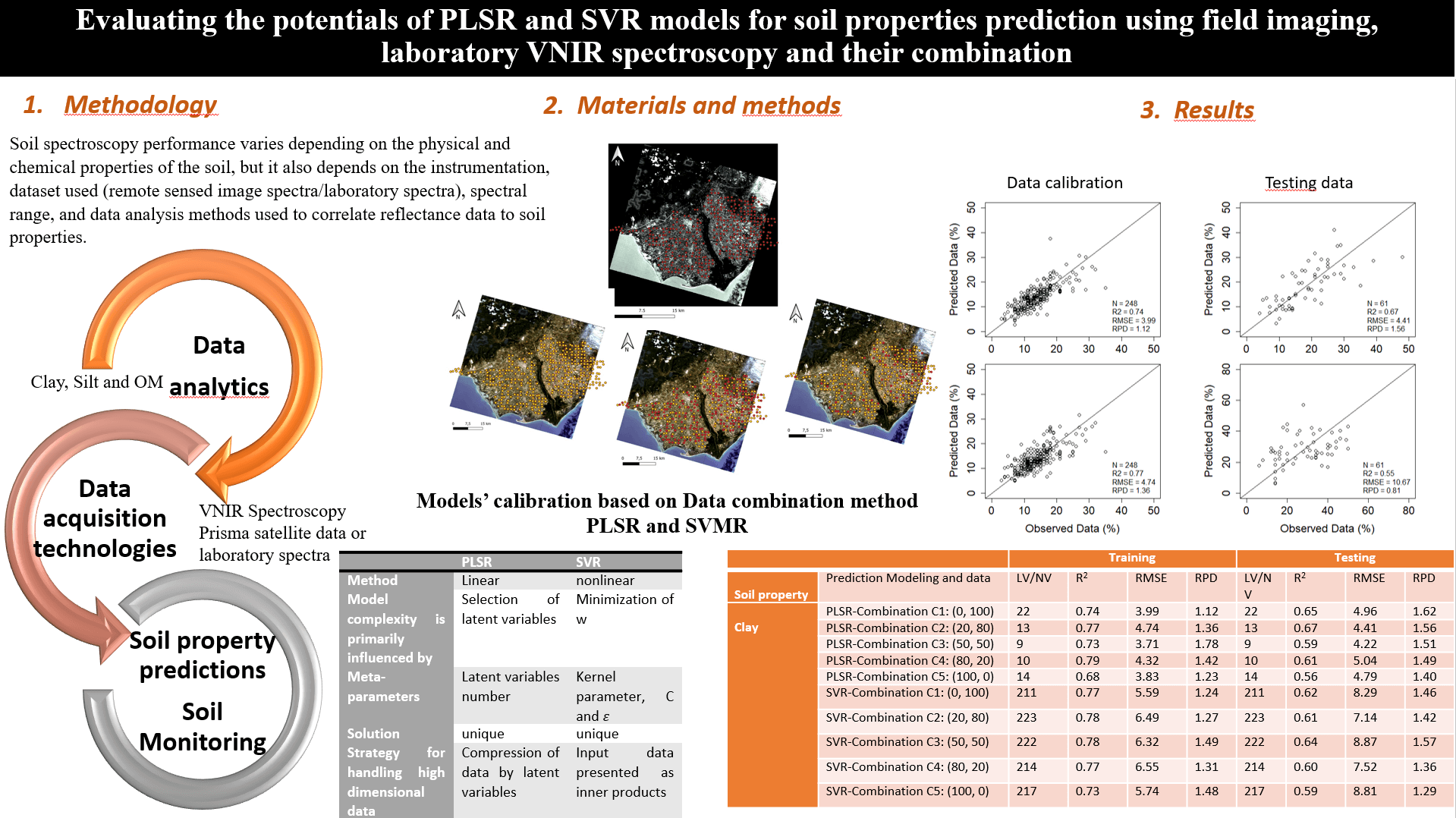
Pedo-spectroscopy has the potential to provide valuable information about soil physical, chemical, and biological properties. Nowadays, we may predict soil properties using VNIR field imaging spectra (IS) such as Prisma satellite data or laboratory spectra (LS). The primary goal of this study is to investigate machine learning models namely Partial Least Squares Regression (PLSR) and Support Vector Regression (SVR) for the prediction of several soil properties, including clay, sand, silt, organic matter, nitrate NO3-, and calcium carbonate CaCO3, using five VNIR spectra dataset combinations (% IS, % LS) as follows: C1 (0% IS, 100% LS), C2 (20% IS, 80% LS), C3 (50% IS, 50% LS), C4 (80% IS, 20% LS) and C5 (100% IS, 0% LS). Soil samples were collected at bare soils and at the upper (0–30 cm) layer. The data set has been split into a training dataset 80% of the collected data (n = 248) and a validation dataset 20% of the collected data (n = 61). The proposed PLSR and SVR models were trained then tested for each dataset combination. According to our results, SVR outperforms PLSR for both: C1 (0% IS, 100% LS) and C5 (100% IS, 0% LS). For Soil Organic Matter (SOM) prediction, it achieves (R2 = 0.79%, RMSE = 1.42%) and (R2 = 0.76%, RMSE = 1.3%), respectively. The data fusion has improved the soil property prediction. The highest improvement was obtained for the SOM property (R2 = 0.80%, RMSE = 1.39) when using the SVR model and applying the second Combination C2 (20% of IS and 80% LS).Graphic Abstract
Keywords
The demographic explosion and overexploitation of resources raise concerns about the future means of achieving food security. The green revolution has demonstrated that chemical agriculture, which relies on the use of fertilizers and pesticides, contributes to environmental degradation. In addition, climate change has intensified land erosion, which may increase by 1.7% for each 1% increase in total precipitation [1]. Therefore, the challenge of the 21st century is to increase agricultural productivity while minimizing ecological harm [2].
Evolutionary applications for sustainable precision agriculture necessarily require knowledge of soil composition to improve soil management Soil accomplishes a variety of important environmental functions that are critical to human survival. For decades, scientists have investigated soil spectroscopy. The recent advances in precision agriculture, as well as the need for spatial assessment of soil properties, have increased interest in this technique. Soil spectroscopy performance varies depending on the physical and chemical properties of the soil, but it also depends on the instrumentation, dataset used (remote sensed image spectra/laboratory spectra), spectral range, and data analysis methods used to correlate reflectance data to soil properties.
Soil property predictions that are quick and accurate can help farmers apply the right amount of fertilizer to maximize yield while lowering costs, as well as create soil property mapping for environmental monitoring.
Monitoring soil status is critical in precision agriculture for adjusting practices like tillage, fertilization, and irrigation. A good understanding of soil characteristics can help growers make better farming decisions and, more broadly, can improve the application of soil management operations, practices, and treatments. Advances in data analytics and data acquisition technologies in environment and agriculture fields have resulted in a plethora of tools for assessing and predicting soil properties. Thanks to advanced automation and decision support tools, it is now possible to predict the impact of climate change on lands. Scientists have conducted many studies in order to better understand and explain the physical, chemical, and biological processes that underpin these various functions. To assess soil properties, a variety of models are now available. Indeed, in the previous two decades, pedometricians have developed linear models such as multiple linear regression, principal component regression and partial least squares regression. Actually, we consider PLSR as the reference calibration method. Nevertheless, because of the complexity of factors that impact simultaneously spectral behavior, the linear model cannot directly interpret the relationship between the spectra and the soil properties. Support Vector Regression is an alternative nonlinear chemometric method for near-infrared spectrometry quantitative analysis [3]. The comparison between linear and nonlinear models is imperative to see which one would provide better prediction performances.
The number of published papers on soil analysis and prediction has increased significantly over the last two decades. These studies have addressed various soil properties; we have listed some of the most relevant key properties for precision farming practices [4]. Soil Organic Matter (SOM) controls soil structural stability [5,6]. Organic Carbone (OC) content depends on the size and capacity of soil microbial populations [7–9]. In addition, Soil Moisture content and clay content are important for plant growth and soil health [10–12]. Moreover, over-fertilization may cause water source contamination by Phosphorus (P) and Nitrogen (N). In this context, environmental monitoring, modeling, and precision agriculture require quantitative data on soil properties [13–15]. The spectral information has proven to be efficient to understand physical and chemical properties of the soil based on absorption and reflectance variation at different wavelength specifically in the NIR region. The Spectral Visible and Near Infrared (VNIR) wavelengths ranges have been proven to be efficient to monitor soil properties [16]. Several soil properties prediction frameworks such as regression techniques have been developed [17–19].
Most prediction approaches are based on linear regression, Principal Component Regression (PCR), Multiple Linear Regression (MLR) and Partial least squares regression (PLSR). A linear regression is applied for each soil property to establish the relation between the dependent variable y and one or more independent variable X. MLR is based on a functional relationship between spectral properties and reference data. PLSR is a multivariate method that applies statistically derived spectral properties to express the derivation of soil properties from spectral ones [20,21]. Based on projecting predictors and response variables into PLSR factors and correspondent scores [22], a multivariate calibration is established. These techniques were used for estimating various soil properties. Reflectance and first-derivative reflectance are commonly used features for predicting Soil Organic Matter [23].
In this study, we calibrated PLSR models. We dispose of soil legacy samples that were previously collected from bare lands. The PLSR model allows the projection of the initial variables into a new space, creating new independent variables (i.e., Latent Variables (LV)).
Selecting the optimal number of LV is critical for developing a robust PLSR model. The optimal number of latent variables was determined using the leave-one-out cross-validation LOO CV method. The number of latent variables is considered optimal when it produces the lowest Root Mean Squared Error RMSE in cross-validation [24]. Both the response variable and the predictor variables have new variables assigned to them. Several indicators are used to assess the model’s prediction performance. The coefficient of determination R2 measures the percentage of the variance in Y explained by variables. In this case, the variable is a linear combination of explanatory variables, as shown in Eq. (1):
where Y denotes the predicted property, bi denotes the model coefficients, and Rλi denotes the reflectance corresponding to the wavelength λi.
The PLSR method analyzes the data based on several noisy collinear features [25,26]. The Principal Component Analysis (PCA) provides a base for VNIR spectroscopy technique in combination with PLS regression analysis [27,28]. It is a practical solution for depicting the presence of outliers in the spectral data of soil samples. This solution, known as latent variable regression, allows the resolution of spectral data into a set of orthogonal components which will be most representative of the variability in the initial data [29].
1.2 Support Vector Regression Model
Machine learning has been widely used for remotely sensed image analysis and classification [30,31]. Support Vector Regression SVR model has demonstrated to be efficient in this particular research field. Even when using a small number of training samples [32]. This predictive technique has the potential to achieve a high accuracy and a strong generalization ability. SVR models also have the virtue to handle multivariate high-dimensional spaces [31].
SVR is a supervised learning based on estimating a functional relationship
C is the error penalty in the optimization problem and is described as follows:
After the tuning process, we set the SVR hyperparameters as follows:
Type: eps-regression (indeed, svm can be used for classification or for regression), epsilon value was set to 0.1 (intensitive-loss function), scale = TRUE (data will be centered and scaled), kernel = ‘radial’ (the kernel used in training and testing), gamma = 1/(data dimension) (parameter needed for all kernels), cost = 1 (cost of constraints violation), na.action = na.omit (reject the missed values).
The equation number (4) demonstrates the formula of the SVR model:
where
We should underline that the radial basis function (RBF) kernel is one of the most used kernel functions.
In addition, the size of the neighborhood surrounding a support vector, which affects predictions for future samples, is controlled by the kernel width,
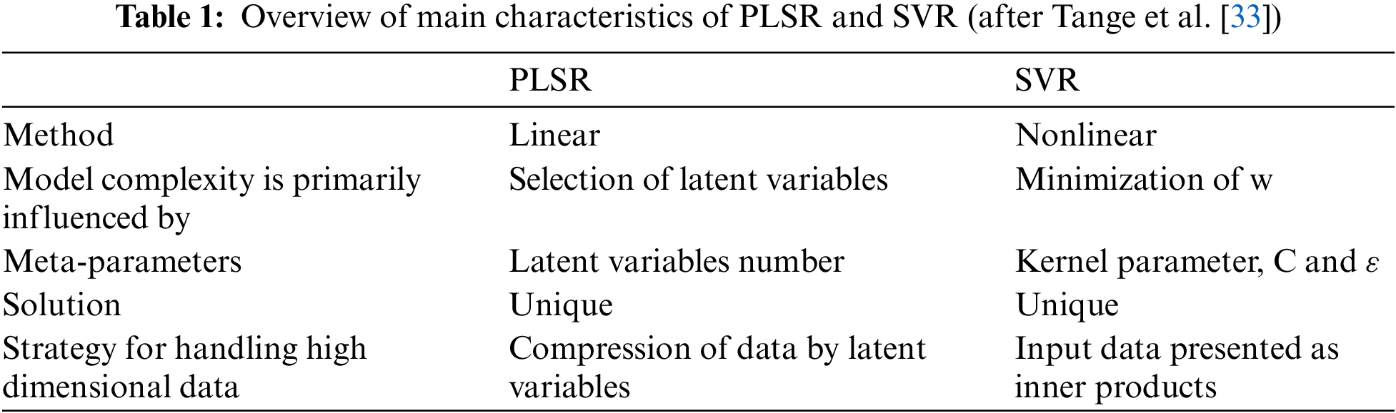
Table 1 outlines the main characteristics of PLSR and SVR models.
According to Vaudour et al. [34], the predictive ability of PLSR models could be classified into three ranges: low, medium and high. The model evaluation is based on: the coefficient of determination R2, the Root Mean Squared Error (RMSE) and on the Residual Prediction Deviation (RPD). Based on RPD and R2, Chang et al. [35] and Viscarra Rossela et al. [36] grouped the predicted values of soil properties into categories A to C, respectively, (RPD > 2.0, 0.8 < R2 < 1.0), (1.4 < RPD < 2.0, 0.5 < R2 < 0.8) and (RPD < 1.4, R2 < 0.5). As previously found by Vaudour et al. [34], the predictive capacity presented by a model property may vary from one region to another.
The quantitative assessments for several soil properties need the exploitation of reflectance spectrum in the visible 400–700 nm, near-infrared 700–1000 nm and shortwave-infrared 1000–2500 nm (VNIR–SWIR) used from various domains (spectroscopy and imaging spectroscopy) as devoted by many studies [37–44]. As previously found by Ben-Dor et al. [45], the research results of the use of Digital Airborne Imaging Spectrometer DAIS 7915 which is a 79-channel high-resolution optical spectrometer that collects information from the Earth’s surface in the 0.4–12.3 μm wavelengths region, hyperspectral airborne sensor to 1 map organic matter, soil field moisture, soil saturated moisture, and soil salinity are promising. Still, the author deduced the limited quality of the used hyperspectral airborne sensor (DAIS-7915).
While various investigations on soil properties have been undertaken, they have focused on particular soil properties, such as SOM, SOC in the VNIR, and Mid-InfraRed (MIR) [46,47]. The VNIR soil properties assessment is less costly and more accurate because water absorption does not affect it. Conversely, soil moisture significantly influences MIR spectroscopy bands. For this reason, it is difficult to embed them into portable devices [47].
The aim of this study was to assess the performance of linear PLSR and non-linear SVR regression models for predicting several soil properties while using and comparing various combinations of VNIR field imaging spectroscopy: notably hyperspectral PRISMA data and VNIR soil samples laboratory spectroscopy.
2.1 Data Collection and Study Area
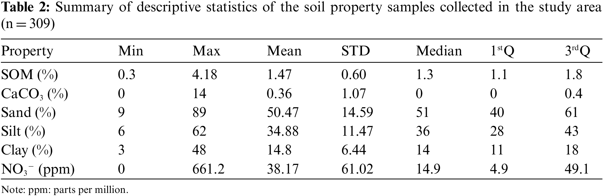
Soil samples were originated from the farmlands surrounding the Nestos River, lying in the region of Eastern Macedonia and Thrace (North-Eastern Greece) (Fig. 1). The study cover area covered of approximately 600 square kilometers [48]. The geology of this area is primarily defined by the river’s alluvial deposits. It is a relatively flat area, with an altitude ranging from 15 to 90 meters and a slope of less than 4%. We collected soil samples between April and June of 2015. In Table 2 we summarized the statistics of the measured soil properties (SOM, CaCO3, Sand, Silt, Clay and NO3−). Soils in this area are mostly sandy with a moderate organic matter content. According to World Reference Base (WRB) taxonomy, a large number of the collected soil samples belong to Fluvisols and Leptosols classes. In this research, the granulometric fractions of each soil sand, silt, and clay are used to determine the soil sample textures. The idea behind this was to use texture as a relevant indicator of soil functional properties notably: water retention capacity, drainage efficiency, root development, soil aeration, microbiome biodiversity, etc. SOM has a wide range of beneficial effects on soil physical and chemical properties as well as, its ability to provide regulatory ecosystem services. SOC management through sustainable agricultural and land use practices is currently a widely accepted strategy. Nitrates are a form of bioavailable nitrogen for plants. Nevertheless, in the soil, nitrates are highly mobile. Assessing the soil nitrate levels help in rationalizing nitrogen fertilization and reducing the amount of pollution caused by excess nitrogen runoff into the environment.
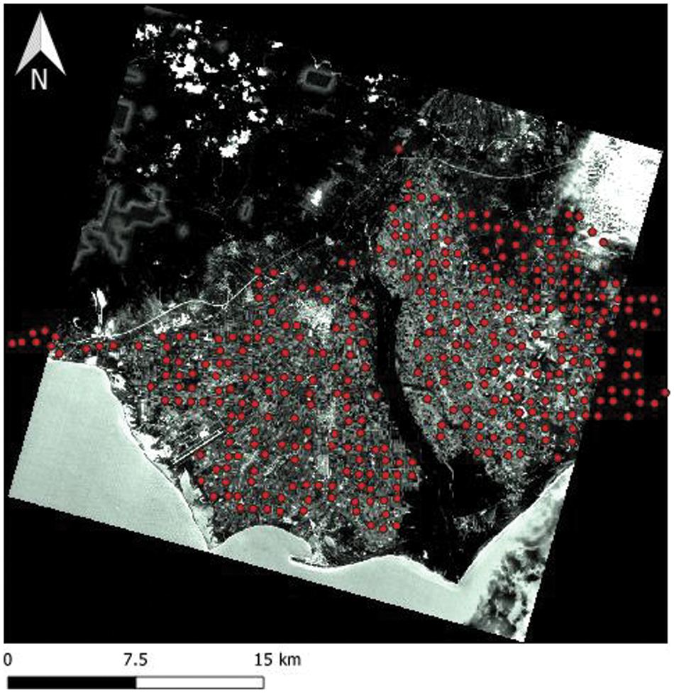
Figure 1: Field sampling points in the study area (base map PRISMA satellite image), Hyperspectral imagery was acquired for the Greece area on May 26th, 2021
The study area is located between 40° and 42° in latitude and between 24° and 25° in longitude. A total of 309 soil samples were collected, in the period between April and June 2015, from the upper layer (0–30 cm) depth.
In this study, we investigated the use of Partial Least Squares Regression (PLSR) and Support Vector Regression (SVR) to predict soil properties using spectroscopic filed images, laboratory data and the combination of both datasets.
The purpose of developing a regression model is to map the soil properties in our geographic area. The challenge is that it is difficult, if not impossible, to “visit” the entire investigation region if it is large. Consequently, the approach involves calculating soil properties based on collected samples and then extrapolating to the full area [49]. It is necessary to establish a relationship between some known variables (x1, x2,…, xn) and the property to be predicted, y, at all points within the area. This is known as the property model: P = f (x1, x2,…, xn), where P is the property under study and “f” is the model obtained. Based on the values of the property P, this relationship is then generalized to all points within the zone using the collected samples.
Several studies have shown that various soil properties can be predicted using laboratory spectra and remotely sensed spectral data. However, the regression model calibrated based on laboratory spectra is, most often, more accurate than the regression model calibrated based on image spectra. Nevertheless, nowadays, image spectra data has become more accessible, more available, and less expensive than laboratory spectra. For large-scale characterization of soil properties, the main goal of this study was to contribute to answering the following question: How could we widespread the exploitation of point laboratory spectra for digital soil properties mapping? Using the fusion strategy, we investigated the modeling performance based on combining the SL and the SI data.
The role of the explanatory variables (x1, x2, …, xn) will be determined by combining remotely sensed images and spectroscopic laboratory measurements in a fusion scheme. Target property is the existence of a certain soil constituent/material (carbon, clay, etc.) or a phenomenon (pH, Electrical Conductivity, etc.). In fact, to some extent, it is assumed that there is a relationship between the investigated property and the soil reflectance spectrum shape.
Therefore, to improve the prediction performance, we propose a fusion scheme based on randomly combining the SL and the SI data by exploiting the reflectance spectrum in the completely spectral ranges VNIR (400–2500 nm).
In a certain manner, 900, 1400, and 2200 nm wavelengths are peaks of absorption of water. At these spectrum wavelengths, soil moisture overlaps or masks the effect of the soil’s target properties. We expected that PLSR and SVR models attribute low weights to these wavelengths.
We dispose of 309 legacy soil samples. These samples were randomly divided in the respective proportions 80% and 20%, into a training data set (n = 248) and a testing data set (n = 61). Thereafter, using both the spectral image SI database and spectral laboratory SL database, we created and compared ten training models (based on five same combinations of SI and SL data sets for PLSR and SVR)). Therefore, the laboratory spectra were resampled to match the dimension of Prisma image spectra. Thus, we get the same number of predictor variable. These combinations are as follows:
(i) C1 (0% SI data set, 100% SL data set), (ii) C2 (20% SI, 80% SL), (iii) C3 (50% SI data set, 50% SL data set), (iv) C4 (80% SI data set, 20% SL data set) and (v) C5 (100% SI data set, 0% SL data set). We should underline that to extract the SI from the PRISMA image at the soil sampling geo-referenced locations; we used the sample raster values in raster analysis tools under the Qgis software. Besides, to ensure that we have collected spectra in bare soils, we have calculated NDVI. All sampled pixels had NDVI values ranging between 0 and 0.22.
As presented in Fig. 2, we created training datasets by combining image and laboratory scanned spectra in five distinct ratios: 0%, 20%, 50%, 80%, and 100% image spectra and 100%, 80%, 50%, 20%, and 0% laboratory spectra. For each soil property, in order to determine which is the best performing model, we have calculated the prediction metrics (R2, RMSE and RPD), which can be obtained from the following equations:
where SSreg SSres and SStot denote, respectively the Sum squared of regression for the explained variation of the target variable, the sum squared of regression for the non-explained variation of the target variable (residual sum of squared) and the total sum squared of regression for variation of the target variable (SStot = SSreg + SSres).
where N denotes the number of explained variables, ei denotes the observed value and êi denotes the predicted value.
where sd denotes the standard deviation and SEP denotes the standard error prediction.
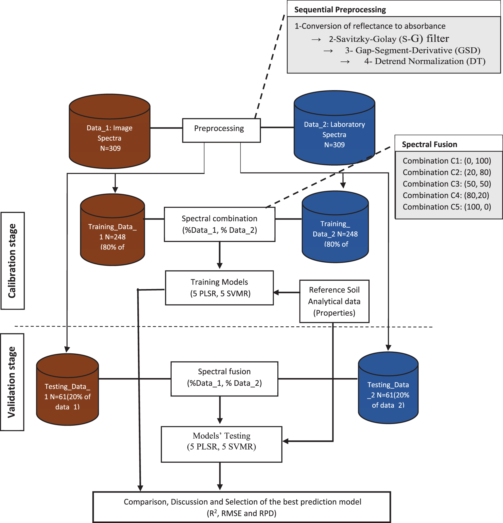
Figure 2: Chart flow of the adopted methodology
2.3 Hyperspectral PRISMA Image Data Acquisition and Processing
PRISMA project (PRecursore IperSpettrale della Missione Applicative, i.e., Italian Hyperspectral Precursor of Operational Mission), aims to develop a small satellite mission entirely in Italy for the monitoring of natural resources and atmospheric characteristics (information on land use and the state of crops, soil mixing, etc.). Hyperspectral imagery was acquired for the Greece area on May 26th, 2021. PRISMA mission also provides standard data acquisition products free of charge to the scientific community, within a short time to process the various related applications to the quality and protection of the environment, sustainable development, climate change, etc. The new satellite PRISMA was launched on the 22nd of March 2019 with an operational lifetime of 5 years [50]. PRISMA images are characterized by a continuum of 240 spectral bands with 10 nm spectral resolution over the spectral region of 400 to 2500 nm, 66 in the Visible Near Infra-Red (VNIR) and 173 in the Short Wave Infra-Red (SWIR) spectrum and acquired at 30 m spatial resolution with approximate 200∶1 Signal to Noise Ratio. The mission’s goal is to determine whether the PRISMA sensor can be successfully used to monitor natural resources and atmospheric characteristics, as well as to assess potential new applications for environmental risk management and land observation [51–54].
The combination of hyperspectral and panchromatic products allows to recognize of the physical-chemical and geometric characteristics of the target of interest within a scene and has the potential to make significant contributions to forest analysis, precision agriculture, water quality assessment, and climate change research [49].
2.4 Laboratory Spectral Measurement
The soil sample laboratory spectral measurements in the VNIR (400–2500 nm) were recorded according to the GEO-CRADLE SSL standard [55]. The field collected soil samples were scanned using an AgriSpec portable spectrometer for 2151 bands within the 350 to 2500 nm spectral region with a spectral resolution of 1 nm. The protocol requires some preliminary processing of the soil samples [56]. Given that the particle size and water content of the soil sample have a significant impact on the recorded spectrum. Soil samples were air dried then sieved to 2 mm. Each soil sample was measured three times, and the average spectrum was computed for further investigation.
2.5 Models’ Calibration Based on Data Combination Method
The precision of a specific soil property depends on the detection method and type of measurement used, such as laboratory and imaging spectroscopy.
The use of a multi-sensor and data fusion approach to improving information extracted from obtained data will be investigated. SI and SL spectra are related to soil properties in some way, but they differ in spatial resolution, spectral resolution, and acquisition conditions. However, they appear to be the same because they depict the same scene and they are two complementary sources of information.
Besides the availability, accessibility and low cost of image spectra, remote sensing has emerged as a promising tool for rapidly quantifying soil properties with the growing demand for quantitative soil information.
The Kennard–Stone (KS) algorithm [57] was used with the argument metric “mahal” to select the training (80%) and testing (20%), respectively, datasets with 248 and 61 samples. Fig. 2 depicts the various steps considered during the development of training models and testing models.
The same combination dataset was used for all five testing PLSR and SVR models to allow for fair comparison.
The fusion was used at random, taking into consideration the spatial distribution of the samples. Fig. 3 depicts the sample distribution, which is important to avoid over-representation of one geographical area over another. This strategy is used for both training and testing samples.


Figure 3: Spatial distribution of training samples using Spectral samples extraction from Prisma image (red points) and Spectral samples extraction from laboratory (yellow points). Spectral Samples extraction with (a) (0% image spectra and 100% laboratory spectra), (b) (20% image spectra and 80% laboratory spectra), (c) (50% image spectra and 50% laboratory spectra), (d) (80% image spectra and 20% laboratory spectra) and (e) (100% image spectra and 0% laboratory spectra)
Fig. 2 shows the combination methodology for Image Spectra IS (Data set 1) and Laboratory Spectra LS (Data set 2).
3.1 Analytical and Spectral Data Pre-Processing
We detail in this part the statistical analysis of the data properties in order to present the soil composition including the minimum (min), maximum (max), mean (mean), standard deviation (SD), median (median), first Quartile (1stQ) and third Quartile (3rdQ). We used the R package stats for this analysis [58]. CaCO3 property is not considered in the experimentation part as it has missing and aberrant values.
Soil property is predictable by VNIR spectroscopy when it is correlated with chemical specificity, according to [5,6,59]. Indeed, due to the phenomenon’s high variability, the interaction between matter and electromagnetic wavelengths (within the soil spectrum sample) is not directly exploitable.
The performance of soil property predictions using VNIR spectroscopy is evaluated by two statistical feature metrics, which are widely used in the literature.
As our goal is to improve the accuracy and robustness of soil properties prediction, we used the following pre-processing detailed in Fig. 2.
1- We considered two different datasets: PRISMA Spectra Image data (SI) and Spectral Laboratory (SL). The dataset (n = 309) was split randomly, using Kennard-Stone (KS) algorithm into two one training (80% of the samples, N = 248) and one testing sub-datasets (20% of the samples, N = 61).
2- Before building and training the models, a data preparation task was performed with the objective of optimizing the prediction models by applying the following sequence of pre-processing techniques: (i) the conversion of reflectance data into absorbance data (log(1/R), where R represents the reflectance), (ii) the Savitzky-Golay (S-G) smoothing filter (SF), (iii) the Gap-Segment-Derivative (GSD), and (iv) the Detrend Normalization (DT) [56,58,60]. Despite the fact that numerous spectra pre-processing operations had been performed, the combination of the aforementioned operations produced the highest level of precision. Typically, absorption transform is used to identify and remove peaks caused by perturbing factors, as well as to enhance spectral resolution. The Savitzky-Golay derivative as another pre-processing method (SG filter) as a convolution function can be viewed as a vector of convolution integers and a normalization factor cannot be performed with non-numeric data or where there are missing data. To implement the filter, Gap-segment and detrend normalization, we used the R packages prospect, mdatools and mathjaxr. For the model’s implementation, PLSR and non-linear-SVR we used the R packages, pls and e1071. For SVR, we used the Gaussian Radial Basis Function (RBF).
3- The training datasets were used to build the models whereas and the testing datasets were used to assess the models accuracy. Three performance measures are considered namely: Coefficient of determination (R2), the Root Mean Squared Error (RMSE) and the Residual Predictive Deviation (RPD). For each soil property and dataset, the best combination of spectral processing and studied regression models were chosen based on the highest Coefficient of determination (R2) and the lowest Root Mean Squared Error (RMSE). To evaluate the robustness of regression models and based on RPD and R2, Chang et al. [35] and Viscarra et al. [36] grouped the predicted values of soil properties into categories A to C respectively, (RPD > 2.0, 0.8 < R2 < 1.0), (1.4 < RPD < 2.0, 0.5 < R2 < 0.8) and (RPD < 1.4, R2 < 0.5). of datasets. R2 measures the percentage of the variance explained by the regression. In fact, for each property, the range of values highly influences the R2 measure. RMSE is defined as the difference between observed and predicted values. For five combinations of PLSR models and five combinations of SVR models in both training and testing data, we investigate the models’ performance using cited statistical indices.
4- Improve the measured to estimated correlation for the Clay, Silt and OM properties by data fusion
3.2 PLSR and SVR Regression Models
The main goal of this study was to investigate the abilities of PLSR and SVR regression models and evaluate their performance for soil properties estimation and quality estimation by using laboratory spectral data and PRISMA image data (SL and SI).
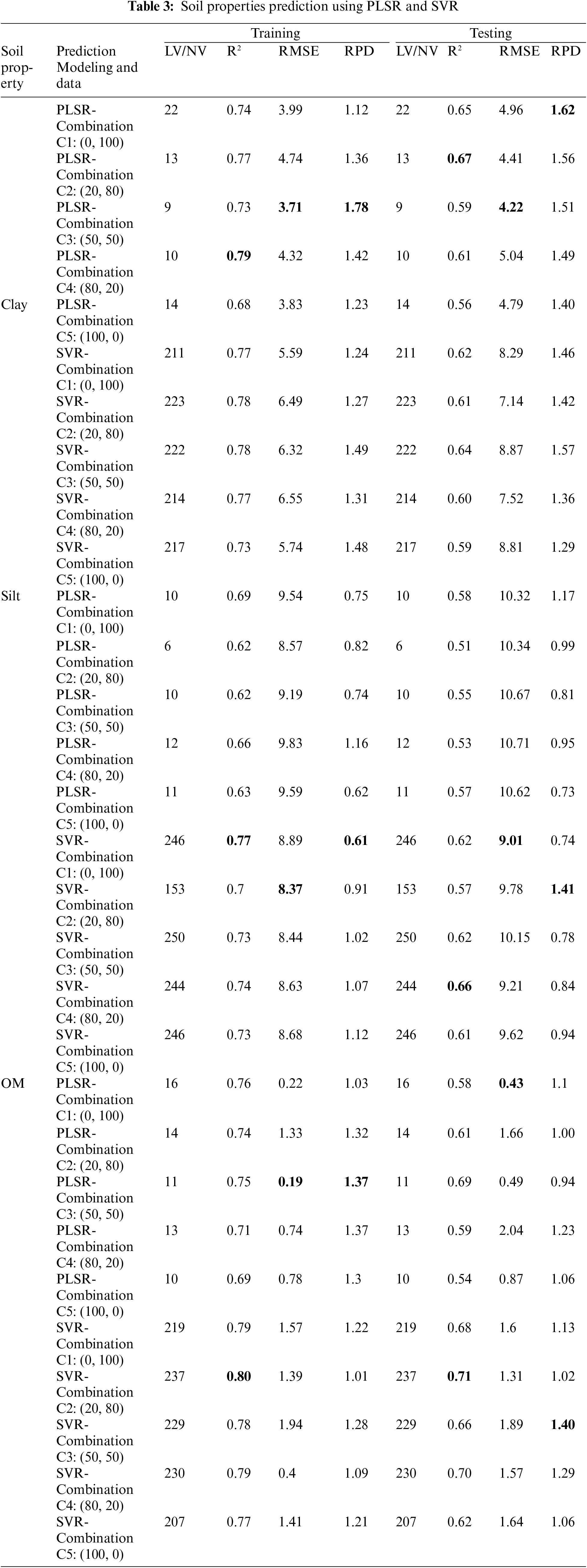
PLSR and SVR results are presented in Table 3 for the ten training models (five combinations PLSR models, five combinations SVR models) with detailed scanning mode (image/laboratory) and ratios of data_1 (image spectra) and data_2 (laboratory spectra): (i) combination C1 (0%, 100%), (ii) Combination C2 (20%, 80%), (iii) Combination C3 (50%, 50%), (iv) Combination C4 (80%, 20%) and (v) Combination C5 (100%, 0%). PLSR and SVR results are presented in Table 3 for ten testing models (five combinations of PLSR models, and five combinations of SVR models) with the same detailed scanning mode (image/laboratory) in the training process.
As proven previously, PLSR and SVR regression models using SL data outperformed those using SI data for almost all properties. This finding is confirmed by several studies. Despite these results, the investigation of spectroscopy images for soil properties prediction has interested several research works. This technology has rich spectral information and has the capability of providing a synoptic view that laboratory spectroscopy cannot provide. The exploration of spectroscopy images led to a fast and low-cost alternative to standard procedures for predicting soil properties with acceptable performance.
A randomly established sampling having real analytical values was adopted to evaluate the prediction results of models developed with laboratory and image spectra. In the following experimentation, we considered only the Silt, Clay and SOM properties.
For Combination C4 (80%, 20%), Training, PLSR model provides the most accurate estimation for Clay (R2 = 0.79, RMSE = 4.32, RPD = 1.42) (Table 3, Fig. 4) and the lowest estimation accuracy for Silt in Combination C2 (20%, 80%) and Combination C3 (50%, 50%) respectively (R2 = 0.62, RMSE = 8.57, RPD = 0.82) and (R2 = 0.62, RMSE = 9.19, RPD = 0.74) (Table 3, Fig. 4).
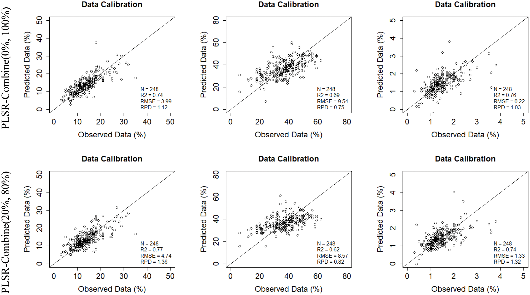
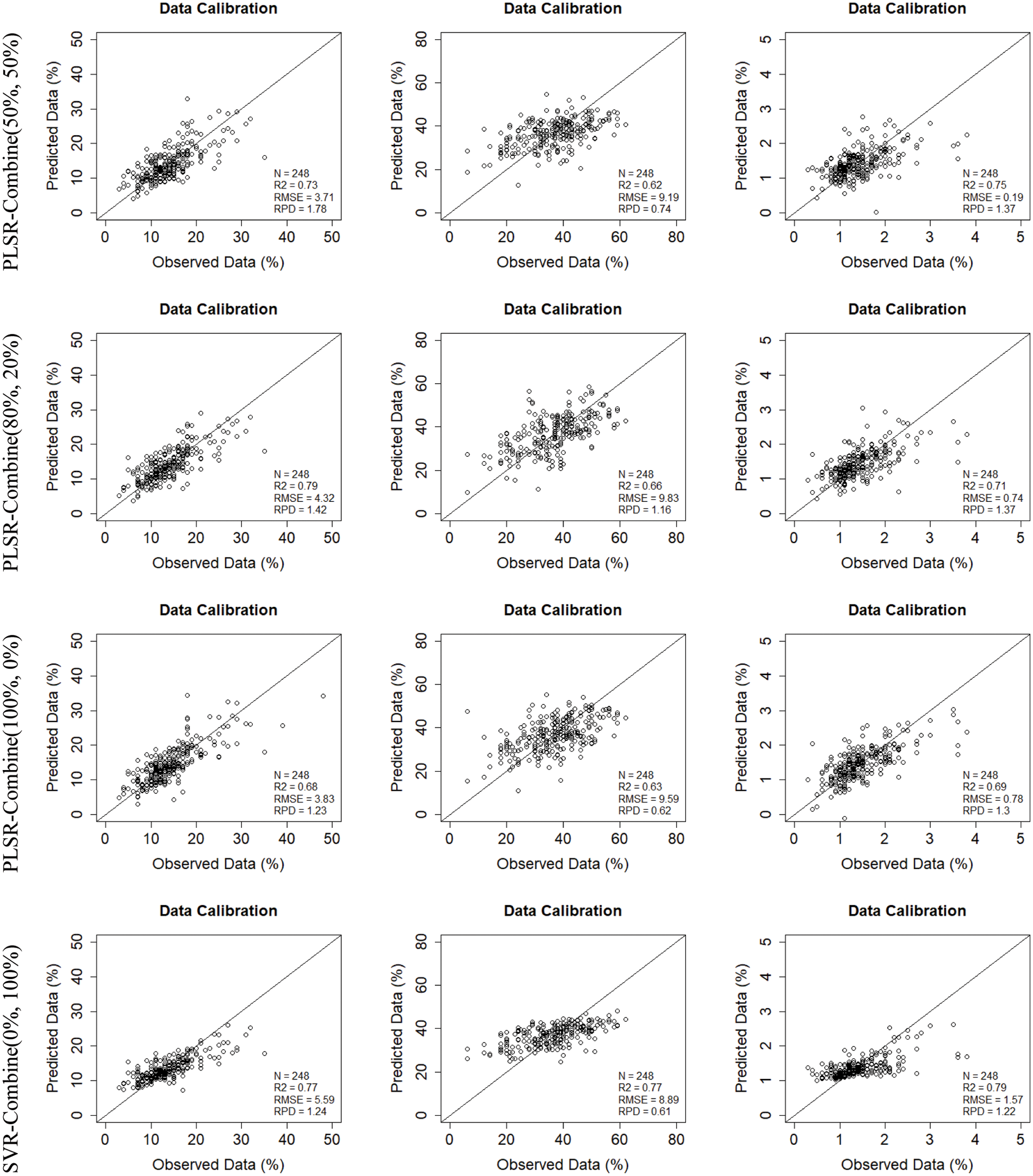
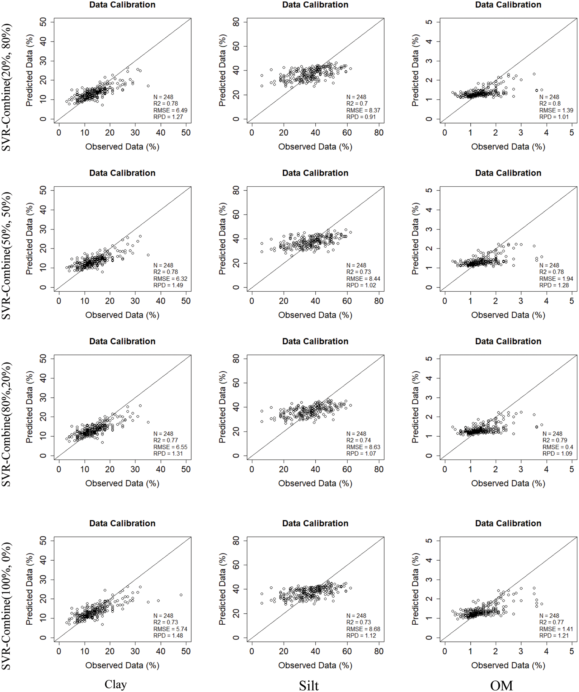
Figure 4: Measured vs. predicted properties for training data using ten training models (five combinations PLSR models, five combinations SVR models) with detailed scanning mode (image/laboratory) and ratios of data_1 (image spectra) and data_2 (laboratory spectra): (i) Combination C1 (0%, 100%), (ii) Combination C2 (20%, 80%), (iii) Combination C3 (50%, 50%), (iv) Combination C4 (80%, 20%) and (v) Combination C5 (100%, 0%)
For Combination C4 (80%, 20%), training SVR model provides the most accurate estimation for OM (R2 = 0.80, RMSE = 1.39, RPD = 1.01) (Table 3, Fig. 4)) and the lowest estimation accuracy for Silt in Combination C2 (20%, 80%) (R2 = 0.70, RMSE = 8.37, RPD = 0.91) (Table 3, Fig. 4).
Predicting performance depends on the measurement mode, for example, the PLSR and SVR results for all fusion processes by combining Prisma Image and Laboratory spectra data outperformed PLSR and for all soil properties predictions except for the case of Clay prediction using the PLSR model in Combination C4 (80%, 20%) which slightly outperformed SVR in the same combination.
The scatterplots in Figs. 4 and 5 presented the measured vs. predicted properties respectively for training and testing data. Generally, for the PLSR prediction model, Clay and SOM properties are mostly close to the diagonal, which presents a visual fitting of the prediction model. Silt is scattered around the diagonal.
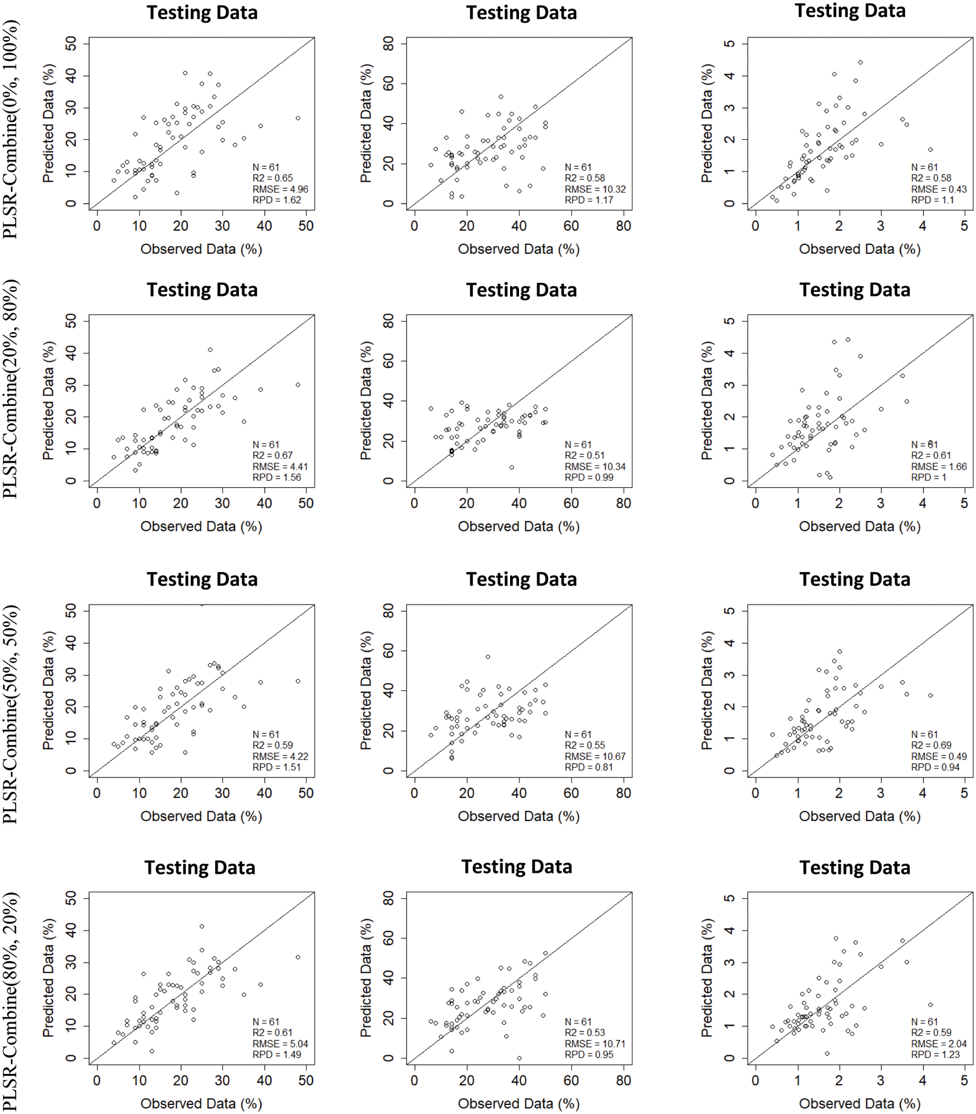
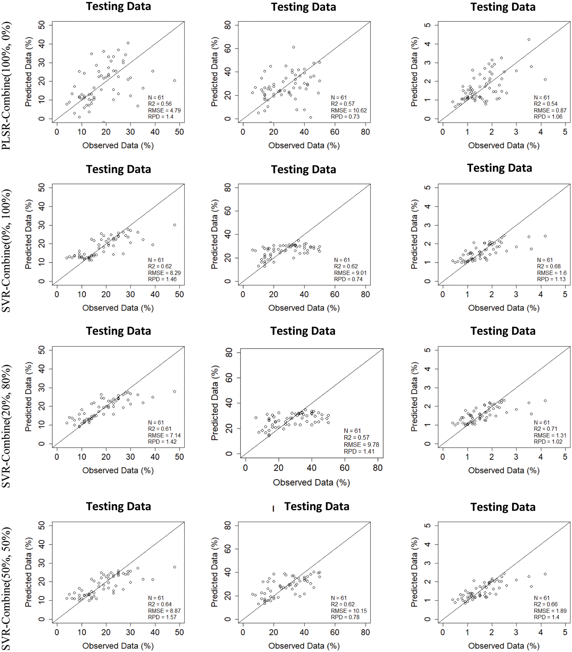

Figure 5: Measured vs. predicted properties for testing data using ten testing models (five combinations PLSR models, five combinations SVR models) with detailed scanning mode (image/laboratory) and ratios of data_1 (image spectra) and data_2 (laboratory spectra): (i) Combination C1 (0%, 100%), (ii) Combination C2 (20%, 80%), (iii) Combination C3 (50%, 50%), (iv) Combination C4 (80%, 20%) and (v) Combination C5 (100%, 0%)
Despite the various methodological decisions that could influence the performance of the prediction model, the purpose of this study is to predict three soil properties using VNIR spectroscopy. We aimed to predict Silt, Clay and SOM. SOM and Silt are, in fact, important soil properties and have crucial roles in agricultural practices.
To estimate these properties, the trained models on SL and SI, provide accurate prediction especially with the SVR models.
The development of a reliable and accurate prediction model is not a panacea. In particular, using a laboratory in conjunction with a satellite database for the prediction model should be done carefully, because there is a mismatch between the laboratory spectra and the Prisma Hyperspectral satellite spectra. In this study, we look for laboratory conditions to overcome the disparity between these two databases in order to use the image spectra:
• In terms of spectral resolution, a sub-sampling was established because laboratory spectra detail covers the VNIR region with very fine spectral resolution; 1 nm, and image spectra detail cover the VNIR region with 10 nm.
• We can only extract information about the topsoil. Besides, the upper layer of soil is not always directly visible by satellite. In our study, Prisma Hyperspectral imagery for the Greece area was acquired on May 26, 2021, and soil samples were collected between April and June of 2015 and air dried in the laboratory. Depending on the time of year and period, the soil may or may not be riddled with weeds or plantations that can disturb the spectral pattern.
• The L2A correction level is present in the Prisma image. It includes geometric corrections for distortion effects, as well as geocoding and georeferencing. The radiometric corrections are processed using photon effect attenuation and a cloud-covered mask on pixels.
SVR outperformed PLSR in all prediction results. Furthermore, finding suitable methods to deal with diverse soil spectra chemometrically is challenging. As a linear multivariate regression model, PLSR is unaffected by collinearity [61] and it allows us to determine the best relationship between chemical compositions and spectra by applying a rotated PCA. Nevertheless, PLSR assumes the linearity between soil properties and spectral characterization. This assumption goes against the edaphically diverse soil composition [62] and the huge frequency spectral variability of soil reflectance in VNIR spectroscopy. The encouraging results consolidate the ability of non-linear SVR model to predict soil properties compared to a linear model such as PLSR.
Laboratory spectra have notably demonstrated the potential for predicting soil properties.
Actually, there is a need to derive improved soil information based on remote and proximal sensing data. To predict soil texture fractions (Sand, Silt and Clay), organic carbon (OC), Calcium Carbonate (CaCO3), pH, and Electrical Conductivity (EC), Kopačková et al. [56] have used an already existing standardized Soil Spectral Library (SSL), across the VIS-NIR-SWIR spectral region range (350–2500 nm) which comprises 1760 soil samples from 9 different countries. They have focused their investigation on a derivation of spectral data that served for soil properties prediction based on an optimal pair of spectral pre-treatments and the combination of two samples selection criteria notably: the geographical proximity and the spectral similarity to generate local subsets. Nevertheless, our approach combines two sources of hyperspectral data notably laboratory proximal and remote sensing image data collected in the same local area that were possible with advanced remote sensing data such as PRISMA data.
Whereas, for large areas, this technique requires the use of more resources including laboratory personnel, equipment and time. Besides, quick and low-cost techniques are required to replace traditional measuring methods. For this purpose, combining image and laboratory spectroscopy can be used for agricultural decision profitability.
With the aim of being able to take max advantage of Prisma spectral data, we look for laboratory conditions to overcome the disparity of these two databases (SI and SL). We can note that R2 values are nearly the same, despite the fact that the laboratory spectra should have a highly better result. The low variability of the soils in this region can explain this result. Furthermore, because the Prisma image was acquired during the dry season (May 26th, 2021), we overcame the humidity perturbance factor that can distinguish between Prisma image and laboratory spectra results. Furthermore, spectral data acquired with image field VNIR spectroscopy at the pixel level is more representative of the real field conditions than spectra acquired in laboratory on handled, air dried, then sieved and scanned soil samples, in three replications.
While based on the RMSE values, the potential of the PRISMA imagery dataset for estimating SOM property (RMSE = 1.3) is slightly better than the potential of the laboratory dataset (RMSE = 1.42).
The implications of these findings for remote estimation of soil properties are numerous. First, these results show that spectral resolution has an effect on PLSR and SVR performance in estimating the soil properties studied. Furthermore, image spatial resolution has an effect on the spectral estimation of individual soil properties.
PLSR and SVR with the laboratory spectra yielded accurate estimations for Clay and OM but less satisfactory for Silt. For this property, the R2 values were higher than those resulting from the Image spectra. But the RPD values were lower than those resulting from both PLSR and SVR with the image spectra except in the case of silt.
With image spectra, the PLSR testing was satisfactory for Clay with RPD > 1.5, implying that some soil properties can be predicted with hyperspectral data with good accuracy.
SOM can be predicted accurately using the SVR model when combining laboratory and image spectra with respectively the ratios 80% and 20%. It can be noted that there were no significant differences between the other combined data.
PLSR had the poorest prediction for Silt for image spectral, laboratory spectra and for all the combination schemes. A large difference between some predicted and measured values for three selected soil properties Clay, Silt and OM (Figs. 4 and 5), is justified by the fact that a PRISMA pixel is 30 by 30 m2. Each sample from a homogeneous 30 by 30 m2 area must be representative.
Soil property prediction performance may be improved by analyzing and selecting a prediction model and adequate data.
This paper makes use of the PLSR and the SVR algorithms to predict several soil properties from laboratory and field imaging (PRISMA data) spectra and the combination thereof. The dataset used is the open Greece GEO-CRADLE Soil Spectral Library. We developed a deep soil properties prediction from several preprocessing and processing scenarios.
The impact of spectral and spatial resolutions on LS and IS data is examined using PLSR and SVR models. In addition, to improve the estimation results, a combination scheme based on a mix of the LS and IS data was considered. Investigating modeling methodologies in VNIR enables for more effective use of spectral data to predict soil parameters [63,64].
The outcomes of our research were to demonstrate the regression dependencies on both the soil properties and the type of data. The hyperspectral space-borne sensor provides almost as good results as the laboratory spectra. The SVR nonlinear prediction model has better performance than PLSR linear prediction model in the VNIR. This research provides a practical demonstration that nowadays, soil properties prediction can be done using laboratory, field imaging spectra data and combined spectra dataset. Meanwhile, the combination scenario will be more appealing if it is based on the spectra’s similarities criteria and provides a rigorous quantitative weighting between laboratory spectra and image spectra datasets.
Acknowledgement: The authors would like to acknowledge the Princess Nourah bint Abdulrahman University Researchers Supporting Project number (PNURSP2023R196), Princess Nourah bint Abdulrahman University, Riyadh, Saudi Arabia. Also, authors would like to thank the reviewers for taking the time and effort necessary to review the manuscript. We sincerely appreciate all valuable comments and suggestions, which helped us to improve the quality of the manuscript.
Funding Statement: This work is supported by Princess Nourah bint Abdulrahman University Researchers Supporting Project number (PNURSP2023R196), Princess Nourah bint Abdulrahman University, Riyadh, Saudi Arabia.
Conflicts of Interest: The authors declare that they have no conflicts of interest to report regarding the present study.
References
1. Nearing, A. M., Pruski, F., O’Neal, M. R. (2004). Expected climate change impacts on soil erosion rates: A review. Journal of Soil and Water Conservation, 59(1), 43–50. [Google Scholar]
2. Delgado, J. A., Short Jr., N. M., Roberts, D., Vandenberg, B. (2019). Big data analysis for sustainable agriculture on a geospatial cloud framework. Frontiers in Sustainable Food Systems, 3(54), 1–13. DOI 10.3389/fsufs.2019.00054. [Google Scholar] [CrossRef]
3. Chen, H., Xu, L., Jia, Z., Cai, K., Shi, K. et al. (2017). Determination of parameter uncertainty for quantitative analysis of shaddock peel pectin using linear and nonlinear near-infrared spectroscopic models. Analytical Letters, 51(10), 1564–1577. DOI 10.1080/00032719.2017.1384479. [Google Scholar] [CrossRef]
4. Nabi, A., Narayan, S., Afroza, B., Mushtaq, F., Mufti, S. et al. (2017). Precision farming in vegetables. Journal of Pharmacognosy and Phytochemistry, 6(6), 370–375. [Google Scholar]
5. Fidêncio, P. H., Poppi, R. J., de Andrade, J. C., Cantarella, H. (2002). Determination of organic matter in soil using near-infrared spectroscopy and partial least squares regression. Communications in Soil Science and Plant Analysis, 33, 1607–1615. DOI 10.1081/CSS-120004302. [Google Scholar] [CrossRef]
6. Conforti, M., Castrignanò, A., Robustelli, G., Scarciglia, F., Stelluti, M. et al. (2015). Laboratory-based vis–NIR spectroscopy and partial least square regression with spatially correlated errors for predicting spatial variation of soil organic matter content. Catena, 124, 60–67. DOI 10.1016/j.catena.2014.09.004. [Google Scholar] [CrossRef]
7. Morgan, C. L., Waiser, T. H., Brown, D. J., Hallmark, C. T. (2009). Simulated in situ characterization of soil organic and inorganic carbon with visible near-infrared diffuse reflectance spectroscopy. Geoderma, 151, 249–256. DOI 10.1016/j.geoderma.2009.04.010. [Google Scholar] [CrossRef]
8. Vohland, M., Besold, J., Hill, J., Fründ, H. C. (2011). Comparing different multivariate calibration methods for the deter-mination of soil organic carbon pools with visible to near infrared spectroscopy. Geoderma, 166, 198–205. DOI 10.1016/j.geoderma.2011.08.001. [Google Scholar] [CrossRef]
9. Gomez, C., Rossel, R. A. V., McBratney, A. B. (2008). Soil organic carbon prediction by hyperspectral remote sensing and field vis-NIR spectroscopy: An Australian case study. Geoderma, 146, 403–411. DOI 10.1016/j.geoderma.2008.06.011. [Google Scholar] [CrossRef]
10. Morellos, A., Pantazi, X. E., Moshou, D., Alexandridis, T., Whetton, R. et al. (2016). Machine learning based prediction of soil total nitrogen, organic carbon and moisture content by using VIS-NIR spectroscopy. Biosystem Engineering, 152, 104–116. DOI 10.1016/j.biosystemseng.2016.04.018. [Google Scholar] [CrossRef]
11. Vendrame, P. R. S., Marchão, R. L., Brunet, D., Becquer, T. (2012). The potential of NIR spectroscopy to predict soil texture and mineralogy in Cerrado Latosols. European Journal of Soil Sciences, 63, 743–753. DOI 10.1111/j.1365-2389.2012.01483.x. [Google Scholar] [CrossRef]
12. Chen, Y., Gao, S., Jones, E. J., Singh, B. (2021). Prediction of soil clay content and cation exchange capacity using visible near-infrared spectroscopy, portable X-ray fluorescence, and X-ray diffraction techniques. Environmental Science and Technology, 55(7), 4629–4637. DOI 10.1021/acs.est.0c04130. [Google Scholar] [CrossRef]
13. Zhang, T., Lin, L., Zheng, B. (2013). Estimation of agricultural soil properties with imaging and laboratory spectroscopy. Journal of Applied Remote Sensing, 7, 073587. DOI 10.1117/1.JRS.7.073587. [Google Scholar] [CrossRef]
14. Ahmadi, A., Emami, M., Daccache, A., He, L. (2021). Soil properties prediction for precision agriculture using visible and near-infrared spectroscopy: A systematic review and meta-analysis. Agronomy, 11(3), 433. DOI 10.3390/agronomy11030433. [Google Scholar] [CrossRef]
15. Shao, Y., He, Y. (2011). Nitrogen, phosphorus, and potassium prediction in soils, using infrared spectroscopy. Soil Research, 49(2), 166–172. DOI 10.1071/SR10098. [Google Scholar] [CrossRef]
16. Vasques, G., Grunwald, S., Sickman, J. O. (2008). Comparison of multivariate methods for inferential modeling of soil carbon using visible/near-infrared spectra. Geoderma, 146, 14–25. DOI 10.1016/j.geoderma.2008.04.007. [Google Scholar] [CrossRef]
17. Hengl, T., Heuvelink, G. B., Stein, A. (2004). Generic framework for spatial prediction of soil variables based on regression-kriging. Geoderma, 120, 75–93. DOI 10.1016/j.geoderma.2003.08.018. [Google Scholar] [CrossRef]
18. Hengl, T., Heuvelink, G. B. M., Rossiter, D. G. (2007). About regression-kriging: From equations to case studies. Computational Geosciences, 33, 1301–1315. DOI 10.1016/j.cageo.2007.05.001. [Google Scholar] [CrossRef]
19. Keskin, H., Grunwald, S. (2018). Regression kriging as a workhorse in the digital soil mapper’s toolbox. Geoderma, 326, 22–41. DOI 10.1016/j.geoderma.2018.04.004. [Google Scholar] [CrossRef]
20. Sahabiev, I. A., Ryazanov, S. S., Kolcova, T. G., Grigoryan, B. R. (2018). Selection of a geostatistical method to interpolate soil properties of the state crop testing fields using attributes of a digital terrain model. Eurasian Soil Sciences, 51, 255–267. DOI 10.1134/S1064229318030122. [Google Scholar] [CrossRef]
21. Elmannai, H., Naceur, M. S., Loghmari, M. A., AlGarni, A. (2021). A new feature extraction approach based on non linear source separation. International Journal of Electrical & Computer Engineering, 11(5), 4082–4094. DOI 10.11591/ijece.v11i5.pp4082-4094. [Google Scholar] [CrossRef]
22. Stevens, A., van Wesemael, B., Bartholomeus, H., Rosillon, D., Tychon, B. et al. (2008). Laboratory, field and airborne spectroscopy for monitoring organic carbon content in agricultural soils. Geoderma, 144(1), 395–404. DOI 10.1016/j.geoderma.2007.12.009. [Google Scholar] [CrossRef]
23. Wold, S., Sjostrom, M., Eriksson, L. (2001). PLS-regression: A basic tool of chemometrics. Chemometrics and Intelligent Laboratory Systems, 58(2), 109–130. DOI 10.1016/S0169-7439(01)00155-1. [Google Scholar] [CrossRef]
24. Moura-Bueno, J. M., Dalmolin, R. S. D., ten Caten, A., Dotto, A. C., Dematte, J. A. M. (2019). Stratification of a local VIS-NIR-SWIR spectral library by homogeneity criteria yields more accurate soil organic carbon predictions. Geoderma, 337, 565–581. DOI 10.1016/j.geoderma.2018.10.015. [Google Scholar] [CrossRef]
25. Elmannai, H., Loghmari, M. A., Naceur, M. S. (2015). Two levels fusion decision for multispectral image pattern recognition. ISPRS Annals of the Photogrammetry Remote Sensing and Spatial Information Sciences, II(22), 69–74. DOI 10.5194/isprsannals-II-2-W2-69-2015. [Google Scholar] [CrossRef]
26. Mouazen, A. M., Kuang, B., Baerdemaeker, J. D., Ramon, H. (2010). Comparison among principal component, partial least squares and back propagation neural network analyses for accuracy of measurement of selected soil properties with visible and near infrared spectroscopy. Geoderma, 158(1–2), 23–31. DOI 10.1016/j.geoderma.2010.03.001. [Google Scholar] [CrossRef]
27. Niazi, N. K., Singh, B., Minasny, B. (2015). Mid-infrared spectroscopy and partial least-squares regression to estimate soil arsenic at a highly variable arsenic-contaminated site. International Journal of Environmental Sciences and Technology, 12, 1965–1974. DOI 10.1007/s13762-014-0580-5. [Google Scholar] [CrossRef]
28. Haaland, D. M., Thomas, V. E. (1988). Partial least-squares methods for spectral analyses. 1. Relation to other quantitative calibration methods and the extraction of qualitative information. Analytical Chemistry, 60(11), 1193–1202. DOI 10.1021/ac00162a020. [Google Scholar] [CrossRef]
29. Elmannai, H., AlGarni, A. (2020). Classification using semantic feature and machine learning: Land-use case application. TelKomnika, 19(4), 1242–1250. DOI 10.12928/telkomnika.v19i4.18359. [Google Scholar] [CrossRef]
30. Elmannai, H., Salhi, A., Hamdi, M., Sliti, M., Loghmari, M. A. et al. (2019). A new rule-based classification framework for remote sensing data. Journal of Applied Remote Sensing, 13(1), 1–16. DOI 10.1117/1.JRS.13.014514. [Google Scholar] [CrossRef]
31. Elmannai, H., Hamdi, M., AlGarni, A. (2019). Enhanced support vector machine applied to land-use classification. Proceedings of the International Conference on Computing, vol. 1097, pp. 236–244. Riyadh, KSA. DOI 10.1007/978-3-030-36365-9_20. [Google Scholar] [CrossRef]
32. Gill, M. K., Asefa, T., Kemblowski, M. W., McKee, M. (2006). Soil moisture prediction using support vector machines. Journal of the American Water Resources Association, 2, 1033–1046. DOI 10.1111/j.1752-1688.2006.tb04512.x. [Google Scholar] [CrossRef]
33. Tange, R. I., Rasmussen, M. A., Taira, E., Bro, R. (2017). Benchmarking support vector regression against partial least squares regression and artificial neural network: Effect of sample size on model performance. Journal of Near Infrared Spectroscopy, 1–10. DOI 10.1177/0967033517734945. [Google Scholar] [CrossRef]
34. Vaudour, E., Gomez, C., Fouad, Y., Lagacherie, P. (2019). Sentinel-2 image capacities to predict common topsoil properties of temperate and Mediterranean agroecosystems. Remote Sensing of Environment, 223, 11–33. DOI 10.1016/j.rse.2019.01.006. [Google Scholar] [CrossRef]
35. Chang, C., Laird, D. A., Mausbach, M. J., Hurburgh, C. R. (2001). Near-infrared reflectance spectroscopy–Principal components regression analyses of soil properties. Soil Sciences Society of America Journal, 65, 480–490. DOI 10.2136/sssaj2001.652480x. [Google Scholar] [CrossRef]
36. Viscarra Rossela, R. A., Walvoortb, D. J. J., McBratneya, A. B., Janikc, L. J., Skjemstadc, J. O. (2006). Visible, near infrared, mid infrared or combined diffuse reflectance spectroscopy for simultaneous assessment of various soil properties. Geoderma, 131(1), 59–75. DOI 10.1016/j.geoderma.2005.03.007. [Google Scholar] [CrossRef]
37. Bogrekci, I., Lee, W. S. (2005). Spectral phosphorus mapping using diffuse reflectance of soils and grass. Biosystem Engineering, 91(3), 305–312. DOI 10.1016/j.biosystemseng.2005.04.015. [Google Scholar] [CrossRef]
38. Ben-Dor, E., Banin, A. (1990). Near-infrared reflectance analysis of carbonate concentration in soils. Applied Spectroscopy, 44(6), 1064–1069. DOI 10.1366/0003702904086821. [Google Scholar] [CrossRef]
39. Ben-Dor, E., Banin, A. (1994). Visible and near-infrared (0.4–1.1 μm) analysis of arid and semiarid soils. Remote Sensing Environment, 48(3), 261–274. DOI 10.1016/0034-4257(94)90001-9. [Google Scholar] [CrossRef]
40. Palacios-Orueta, A., Ustin, S. L. (1998). Remote sensing of soil properties in the Santa Monica Mountains I. Spectral analysis. Remote Sensing Environment, 65(2), 170–183. DOI 10.1016/S0034-4257(98)00024-8. [Google Scholar] [CrossRef]
41. Ingleby, H. R., Crowe, T. G. (2000). Reflectance models for predicting organic carbon in Saskatchewan soils. Canadian Biosystems Engineering, 42(2), 57–63. [Google Scholar]
42. Thomasson, J. A. (2001). Soil reflectance sensing for determining soil properties in precision agriculture. Transactions of the ASAE. American Society of Agricultural Engineers, 44(6), 1445–1453. DOI 10.13031/2013.7002. [Google Scholar] [CrossRef]
43. Asner, G. P., Heidebrecht, K. B. (2003). Imaging spectroscopy for desertification studies: Comparing AVIRIS and EO-1 hyperion in Argentina drylands. IEEE Transaction of Geoscience and Remote Sensing, 41(6), 1283–1296. DOI 10.1109/TGRS.2003.812903. [Google Scholar] [CrossRef]
44. Schwanghart, W., Jarmer, T. (2011). Linking spatial patterns of soil organic carbon to topography-a case study from south eastern Spain. Geomorphology, 126(1), 252–263. DOI 10.1016/j.geomorph.2010.11.008. [Google Scholar] [CrossRef]
45. Ben-Dor, E., Patkini, K., Banin, A., Karnieli, A. (2002). Mapping of several soil properties using DAIS-7915 hyperspectral scanner data—A case study over clayey soils in Israel. International Journal of Remote Sensing, 23(6). DOI 10.1080/01431160010006962. [Google Scholar] [CrossRef]
46. Lagacherie, P., Baret, F., Feret, J. B., Netto, J. M., Robbez Masson, J. M. (2008). Estimation of soil clay and calcium carbonate using laboratory, field and airborne hyperspectral measurements. Remote Sensing and Environment, 112(3), 825–835. DOI 10.1016/j.rse.2007.06.014. [Google Scholar] [CrossRef]
47. Gholizadeh, A., Boruvka, L., Saberioon, M., Vašát, R. (2013). Visible, near-infrared, and mid-infrared spectroscopy applications for soil assessment with emphasis on soil organic matter content and quality: State-of-the-art and key issues. Applied Spectroscopy, 67, 1349–1362. DOI 10.1366/13-07288. [Google Scholar] [CrossRef]
48. Le Bouler, G., Rogival, M. (2017). Coordinating and integrating state-of-the-art Earth Observation Activities in the regions of North Africa, Middle East, and balkans and developing links with GEO related initiatives towards GEOSS. GEO-CRADLE H2020, 690133. https://cordis.europa.eu/project/id/690133. [Google Scholar]
49. Bartholomeus, H., Schaepman-Strub, G., Blok, D., Udaltsov, S., Sofronov, R. (2010). Estimation and extrapolation of soil properties in the Siberian Tundra, using field spectroscopy. Proceedings of the Conference of Art, Science and Applications of Reflectance Spectroscopy Symposium, pp. 1–10. Boulder. [Google Scholar]
50. Vangi, E., D’Amico, G., Francini, S., Giannetti, F., Lasserre, B. et al. (2021). The New hyperspectral satellite PRISMA: Imagery for forest types discrimination. Sensors, 21, 1182. DOI 10.3390/s21041182. [Google Scholar] [CrossRef]
51. Chiavetta, U., Camarretta, N., Garfı, V., Ottaviano, M., Chirici, G. et al. (2016). Harmonized forest categories in central Italy. Journal of Maps, 12, 98–100. DOI 10.1080/17445647.2016.1161437. [Google Scholar] [CrossRef]
52. Loizzo, R., Guarini, R., Longo, F., Scopa, T., Formaro, R. et al. (2018). Prisma: The Italian hyperspectral mission. Proceedings of the 2018 IEEE International Geoscience and Remote Sensing Symposium, pp. 175–178. Valencia, Spain. DOI 10.1109/IGARSS.2018.8518512. [Google Scholar] [CrossRef]
53. Guarini, R., Loizzo, R., Longo, F., Mari, S., Scopa, T. et al. (2017). Overview of the prisma space and ground segment and its hyperspectral products. Proceedings of the 2017 IEEE International Geoscience and Remote Sensing Symposium (IGARSS), pp. 23–28. Fort Worth, TX, USA. DOI 10.1109/IGARSS.2017.8126986. [Google Scholar] [CrossRef]
54. Busetto, L. P. (2020). An R package for importing PRISMA—v0.1.0. https://github.com/lbusett/prismaread. [Google Scholar]
55. Tziolas, N., Tsakiridis, N., Ben-Dor, E., Theocharis, J., Zalidis, G. (2019). A memory-based learning approach utilizing combined spectral sources and geographical proximity for improved VIS-NIR-SWIR soil properties estimation. Geoderma, 340, 11–24. DOI 10.1016/j.geoderma.2018.12.044. [Google Scholar] [CrossRef]
56. Kopačková, V., Ben-Dor, E. (2016). Normalizing reflectance from different spectrometers and protocols with an internal soil standard. International Journal of Remote Sensing, 37(6), 1276–1290. DOI 10.1080/01431161.2016.1148291. [Google Scholar] [CrossRef]
57. Kennard, R. W., Stone, L. A. (1969). Computer aided design of experiments. Technometrics, 11(1), 137–148. DOI 10.2307/1266770. [Google Scholar] [CrossRef]
58. R Core Team (2016). R: A language and environment for statistical computing. R Foundation for Statistical Computing. https://www.R-project.org/. [Google Scholar]
59. Ben Rabah, Z., Garbia, H., Karray, E., Tounsi, K., Kallel, A. et al. (2019). Hyperspectral analysis for a robust assessment of soil properties using adapted PLSR method. Advances in Remote Sensing, 8, 99–108. DOI 10.4236/ars.2019.84007. [Google Scholar] [CrossRef]
60. Fearn, T. (2008). The interaction between standard normal variate and derivatives. NIR News, 19, 16–17. DOI 10.1255/nirn.1098. [Google Scholar] [CrossRef]
61. Tenenhaus, M., Gauchi, J. P., Menardo, C. (1995). Régression PLS et applications. Revue de Statistique Appliquée, 43(1), 7–63. [Google Scholar]
62. Calderón, F. J., Culman, S., Six, J., Franzluebbers, A. J., Schipanski, M. et al. (2017). Quantification of soil permanganate oxidizable C (POXC) using infrared spectroscopy. Soil Science Society of America Journal, 81, 277–288. DOI 10.2136/sssaj2016.07.0216. [Google Scholar] [CrossRef]
63. Bera, S., Shrivastava, V. K., Satapathy, S. C. (2022). Advances in hyperspectral image classification based on convolutional neural networks: A review. Computer Modeling in Engineering & Sciences, 133(2), 219–250. DOI 10.32604/cmes.2022.020601. [Google Scholar] [CrossRef]
64. Baruah, H. G., Nath, V. K., Hazarika, D. (2022). Remote sensing image retrieval based on 3D-local ternary pattern (LTP) features and non-subsampled shearlet transform (NSST) domain statistical features. Computer Modeling in Engineering & Sciences, 131(1), 137–164. DOI 10.32604/cmes.2022.018339. [Google Scholar] [CrossRef]
Cite This Article
 Copyright © 2023 The Author(s). Published by Tech Science Press.
This work is licensed under a Creative Commons Attribution 4.0 International License , which permits unrestricted use, distribution, and reproduction in any medium, provided the original work is properly cited.
 Downloads
 Citation Tools