A Simple and Efficient Structural Topology Optimization Implementation Using Open-Source Software for All Steps of the Algorithm: Modeling, Sensitivity Analysis and Optimization

1  Introduction

Structural topology optimization aims to find the best distribution of a given material within a structural domain in order to maximize/minimize some objective function. Among the most explored objective functions, the following stand out: stiffness, stress, natural frequency, thermal capacity, buckling, or a combination of these [1]. In recent years, structural optimization has had a great impact on the industry, where several effective approaches have been developed and consolidated. In a general way, structural topology optimization can be classified into two types: one considering discrete elements and the other considering continuous elements. In the discrete elements approach, according to [2], one of the precursors of this approach, the optimal structures are obtained through an extensive search in a predefined set of discrete elements, such as for example beams and trusses discretized in a given domain of analysis, as illustrated in Fig. 1, by [3].

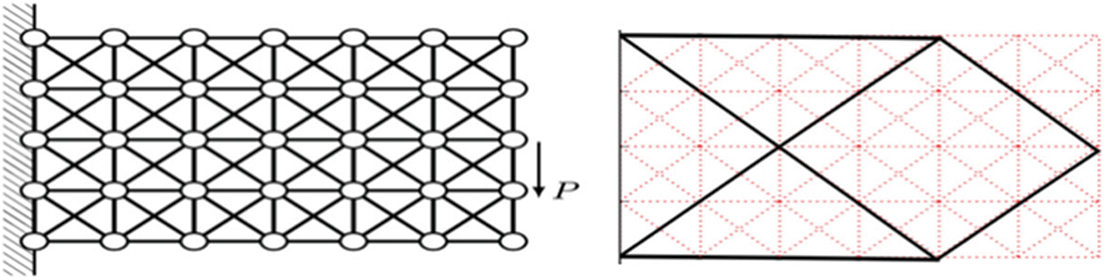
Figure 1: Discrete element and its optimization

In this approach, global optimization methods can be used such as genetic algorithms [4], PSO-Particle Swarm Optimization [5], ACO algorithms-Ant Colony Optimization [6]. On the other hand, discrete methods based on objective function gradients, can be based such as BESO-Bidirectional Evolutionary Structural Optimization [7] or TOBS-Topology Optimization of Binary Structures [8].

In the continuous elements approach, the optimal structures can be found considering an interpolation of the material [9], for each location within a design domain, as illustrated in Fig. 2.

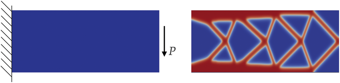
Figure 2: Continuous element and its optimization

Some works have extensive analyzes of the discrete element approach [10,11,12]. The simultaneous optimization of shape and size using a similar approach is done by [13–16]. The continuous element approach has also been applied to numerous optimization problems, such as stiffness problems [17], eigenfrequency problems [18–20], resistance automotive shock [21] and mechanical reliability analysis optimization problems [22,23]. Thus, structural topology optimization is increasingly expanding its space in practical applications in the mechanical, aerospace and civil industries. Currently, researchers in the area tend to use ready-made open-source software components that facilitate the implementation of topology optimization programs. In this context, the reuse of software components for the development of open codes gains relevance and, therefore, has been much explored recently.

Thus, the present work presents a new simple and numerically efficient code for structural topology optimization with only 51 lines of code using open-source software for all stages of the topology optimization problem: modeling, sensitivity analysis and optimization. The elastostatic mechanical problem is discretized by the finite element method using internal FEniCS tools. Sensitivity analysis is performed using the Dolfin Adjoint program. Optimization problem, formulated using SIMP interpolation, are solved using Ipopt optimizer functions. The proposed approach allows users to concentrate on the abstract mathematical formulation of the optimization problem, without spending a lot of effort on computational implementation. Thus, all the code is done in a completely open way, without the need for commercial tools or even without the need to install additional modules. The problem being considered is the minimization of the compliance of 2D and 3D structures.

1.1 Open Programs on STO

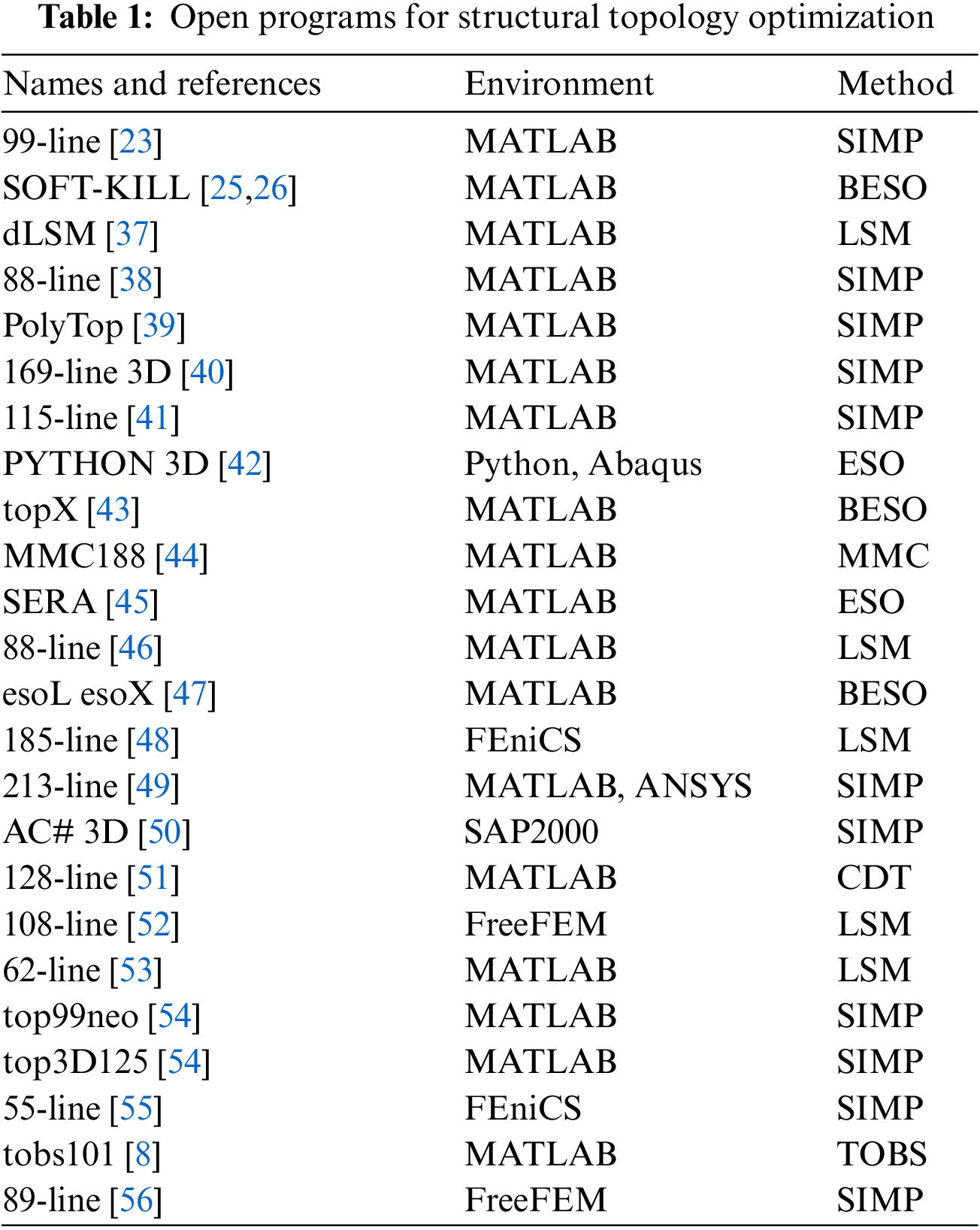
Regarding open programs on structural topology optimization, one of the first open programs was published by [24], a 99 line topology optimization code written in Matlab. As in the present work, Sigmund [24] used the topology optimization approach with the SIMP method-Solid Isotropic Material with Penalization. Open structural topology optimization programs were developed using other approaches such as: ESO-structural evolutionary optimization and BESO - bidirectional evolutionary structural optimization methods [7,25–31], LSM-Level Set Method [32–34], TOBS-topology optimization of binary structures [8], MMC method-moving morphable components [35,36], among others. Table 1 presents a survey with open-source examples on structural topology optimization, describing the name of the code and authors, the programming language used, and the optimization method used.

In the work published by [57], a comprehensive review of educational articles on structural and multidisciplinary optimization, an extensive survey is carried out on works with educational or open codes made by the structural and multidisciplinary optimization (SMO) community, showing mainly the growth of this type of publication in recent years, the number of downloads and even the number of citations. Also in [57], a detailed description of the main characteristics of each work is made, such as topology, dimensioning, optimization, and others. It also provides comparisons and evaluations on the codes of several important aspects, including techniques, efficiency, usability, readability, environment and compatibility, demonstrating the importance and practicality of the value of an educational or open publication in a pedagogical way in dictionary format with specific directions for each theme.

The use of commercial software versus the use of open-source software has very particular characteristics, where the financial factor ends up being predominant. Thus, the objective of this article is to develop computational tools that allow a solid analysis of the finite element method, and that do all the calculations necessary for the topology optimization process and that are free. According to [58], FEniCS [59,60] is a research project that aims to create mathematical methods and software for automated computational mathematical modeling. This means creating easy, intuitive, efficient and flexible software to solve partial differential equations using finite element methods.

In the research carried out by [55], a 55-line code for large-scale parallel topology optimization in 2D and 3D, an open-source code is made using FEniCS, as in the present work, based on the SIMP approach, however, with a different code approach. In their work [55], they opted for the process of replicating the code of works 99-line [24], and 88-line [38], using tools available only in FEniCS, not using the Adjoint method available in Dolfin Adjoint software [61,62,63]. Thus, the use of Euclidean distance matrices is made to vectorize the calculation of distance matrices for the filter and also making use of the optimization algorithm with the standard method of optimality criterion satisfying KKT conditions (Karush–Kuhn–Tucker) with the insertion of a Lagrangian Multiplier being applied to satisfy the sensitivity of its objective function by the bisection method. This type of approach made in [55] has great results. However, it still requires, in addition to the standard FEniCS tools, the use of other programming packages to assemble all of them for finite elements and optimization. Its language is very close to software like Matlab and ends up “losing” a little functionality and high code abstraction available in the FEniCS and Dolfin Adjoint package.

With FEniCS, it is possible to calculate the sensitivities using the adjoint method, which automatically derives the adjoint and tangent discrete linear models from a direct model written in the Python interface, through the Dolfin Adjoint. Thus, the SIMP method can be implemented using a sensitivity analysis based on the adjoint method. In this work, the relative density of each finite element is used as a design variable for the optimization problem. The material interpolation follows a power law, penalizing elements of intermediate density and leading the topology to an optimized binary state of solid and empty material [24,64,65]. Sensitivity analysis, in terms of robustness and efficiency, is one of the great challenges in the field of high-performance scientific computing [66]. Thus, Dolfin Adjoint aims to solve this problem for the case where the model is implemented in the Python interface for FEniCS, where given a differentiable model, employing Dolfin Adjoint involves few changes in the computational code. The linear adjoint, and tangent models exhibit optimal theoretical efficiency where if each direct variable is stored, the adjoint takes from 0.2 to 1.0 times the execution time of the direct model, depending on the structure of the characteristics of the direct problem. If the model direct is performed in parallel, sensitivity calculations are also performed in parallel without modification in Dolfin Adjoint [66].

Finally, when comparing the works listed in Table 1, including those done in FEniCS, most are replications or improvements of the original codes using SIMP or BESO. Thus, in the present work, we use both FEniCS and Dolfin Adjoint in an integrated implementation. The proposed code has the simplest and most objective language, follows the writing of mathematical formulations in a very clear and readable way, simplifying the abstract formulation of the FEM. The Dolfin Adjoint code makes the whole process of differentiating the sensitivities in a simple and direct way with a small number of code lines. Following the similar procedure, the optimization problem is solved using the Ipopt module. Another differential of our code is for 2D and 3D cases, being able to solve relatively large 3D problems, allowing to solve real engineering problems.

Also, considering the programming language used as base, Python, there is no need to install any other numerical/mathematical module. For simulations considering multiplus parallelization processes, due to the programming method and the relationship between the FEniCS and Dolfin Adjoint programs, there is no need to change the code. And finally, so far, it is the code with the fewest lines ever made.

1.2 Finite Element Method Using FEniCS

The implementation of the finite element method was done using the FEniCS platform. The problem must be formulated using functional analysis [67]. FEniCS is a tool capable of solving PDEs by the finite element method, and was designed to make implementations more compact, which is attractive because it uses the abstract formulation of the method [67]. Over the last few decades, much work has been done on the finite element method and in a general way, it is considered that among most of these works there is a format division of the method approach into two categories, the first is an abstract mathematical version of the method and the second is the formulation of engineering “structural analysis” [58]. Thus, the FEniCS software is based on applying the concepts of the first approach, the abstract mathematics of the finite element method. Other works that follow this same approach in the development of the finite element method are done by [68,69].

The formulation can be written using the weighted residuals method of the GALERKIN type, where the solution of a PDE can be obtained considering a nodal polynomial approximation by subdomains. For this, the test functions that are used in FEniCS programs are defined. Test functions belong to certain function spaces that specify the properties of the adopted numerical approximations, [58].

2  Structural Topology Optimization (STO)

Thus, in order to perform structural topology optimization, the problem of minimizing structural compliance (mean sensibility) is defined through an objective function over a domain, according to Eq. (1):

L(v)=∫Ωf.vdΩ+∫∂ΓNT.vdΓ(1)

Being in Eq. (1): L(v) the work of external volume forces f and surface forces T, v represents the test functions, Ω is the domain and ∂ΓN is the portion of the boundary where surface forces are applied.

The equilibrium conditions are considered as constraints of the problem and are given by:

−∇.σ=finΩ(2)

σ.n=TonΓN(3)

Being in Eqs. (2) and (3): σ the Cauchy stress tensor, n represents the external normal direction at ΓN and ∇.σ is the stress divergence, as follows:

∂σxx∂x+∂σxy∂y=−fx(4)

∂σxy∂x−∂σyy∂y=−fy(5)

σxxnx+σxyny=Tx(6)

σxynx−σyyny=Ty(7)

And the following additional restrictions:

∫Ωρ(x)dx≤V(8)

0≤ρ(x)≤1,∀x∈Ω

Since the parameter ρ(x) is the design variable (ρ(x)=1 means presence of material and ρ(x)=0 means absence of material), V, in Eq. (8), it is the volume of the structural domain. The strain displacement relations considering the small elastic deformations of a body Ω can be written as:

ϵ(v)=12(∇v+(∇v)T)(9)

The constitutive equations can be written as:

σ(u)=λtr(ϵ)I+2μϵ(10)

And the linear integral form of the equilibrium conditions can be written as:

a(u,v)=∫Ωσ(u):ϵ(v)dx(11)

Being in Eqs. (9)–(11): u the displacement field, ϵ(v) the linear part of the Green strain tensor, tr is the tensor trace and I is the identity tensor. The Lamé constants are λ and μ according to:

λ=Ev(1+υ)(1−2υ),μ=E2(1+υ)(12)

Being in Eq. (12): E the Young’s modulus and υ a Poisson coefficient.

With this, the variational formulation is summarized in how to find u so that u∈V, where:

a(u,v)=L(v)∀v∈V^(13)

Being in Eq. (13): V a discrete function space and V^ the Hilbert subspace of v admissible functions.

Isotropic elastic material behavior is assumed in the examples of this work. The material distribution ρ(x) is done by updating the material stiffness through compliance minimization, which can be written as follows [9]:

min. L(v)

s.a.:a(u,v)=L(v)∀v∈V^(14)

∫Ωρ(x)dx≤V with 0≤ρ(x)≤1,∀x∈Ω

Thus, a continuous SIMP relaxation is performed, proposed by [9] according to:

E=Emin+(Emax−Emin)ρ(x)p(15)

where E is the modulus of elasticity updated for each element, where Emax is the elasticity of the material used and Emin is a very small “value” attributed to empty regions, in order to prevent the stiffness matrix from becoming singular [38]. The penalty constant p, is adopted equal to 3 [1], for cases of linear elasticity.

3  Density Filter

Due to the choice of a power law for the interpolation of the material, according to Eq. (15), problems of alternating solutions with p=0 and p=1 may arise, which generates a numerical problem of the “checker board” type [70,71,72]. Thus, to alleviate this problem, a density filter is added, which can be implicitly represented by the solution of a partial differential equation of the Helmholtz type with homogeneous Neumann boundary conditions according to [73] and described in Eq. (16).

−Rmin2∇2ψ~+ψ~=ψ(16)

where ψ is the continuous representation of the unfiltered design variable and ψ~ is the filtered design variable. The parameter Rmin plays a similar role to the rmin used in classical filtering approaches that use the SIMP method. In [73] an approximate relationship between the length scales for the classical filter and the Helmholtz approach as Rmin=rmin23 is described.

The solution of Eq. (16) can be written in the form of an integral convolution which is equivalent to the classical filter. In terms of the variational formulation, it is as follows:

−Rmin2∫Ω∇ρ(x)~.∇wdΩ+∫Ω∇ρ(x)~wdΩ=∫Ωρ(x)wdΩ∀w∈W^(17)

where W^ is the Hilbert subspace of w admissible functions.

As observed in the article of [38], the traditional density filter approach accelerates the filtering process if the search procedure is performed only once as a pre-processing step, however, the computational complexity and memory usage are proportional to Rmin2 in two dimensions and Rmin3 in three dimensions, respectively. The Helmholtz filter approach uses the same mesh used to solve equilibrium equations and does not require any additional information, which avoids excessive memory usage. Considering also that the computational cost depends linearly on the length parameter Rmin, for a large filtering radius, mainly in three-dimensional domains, the filtering approach using differential equations should be the preferred choice.

4  Numerical Implementation

Equilibrium equations, Eq. (13), are solved using the finite element method approach using the FEniCS framework, which converts the models described by variational forms into efficient finite element code. The optimization problem described in Eq. (14) is solved using the optimization routines from the Ipopt library [74], which is a software package for large-scale nonlinear optimization that implements an “interior-point” and a “line-search”. The analysis and optimization methods used are suitable for large problems with up to millions of variables and constraints. Sensitivities are calculated by the adjoint method using the Dolfin Adjoint package, which automatically derives the adjoint discrete linear models and tangents of a direct model written in the Python interface for FEniCS.

In Fig. 3 a general scheme of the numerical implementation is shown.

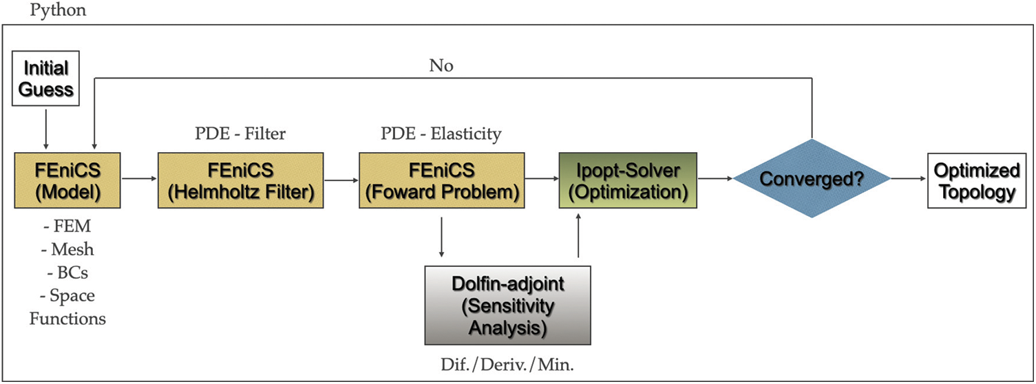
Figure 3: Numerical implementation routine

The code base is presented based on the classic example of a cantilever beam as shown in Fig. 4.

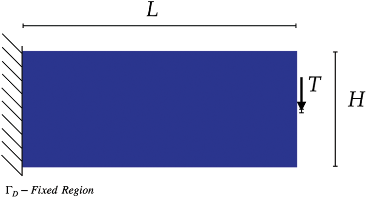
Figure 4: Cantilever beam

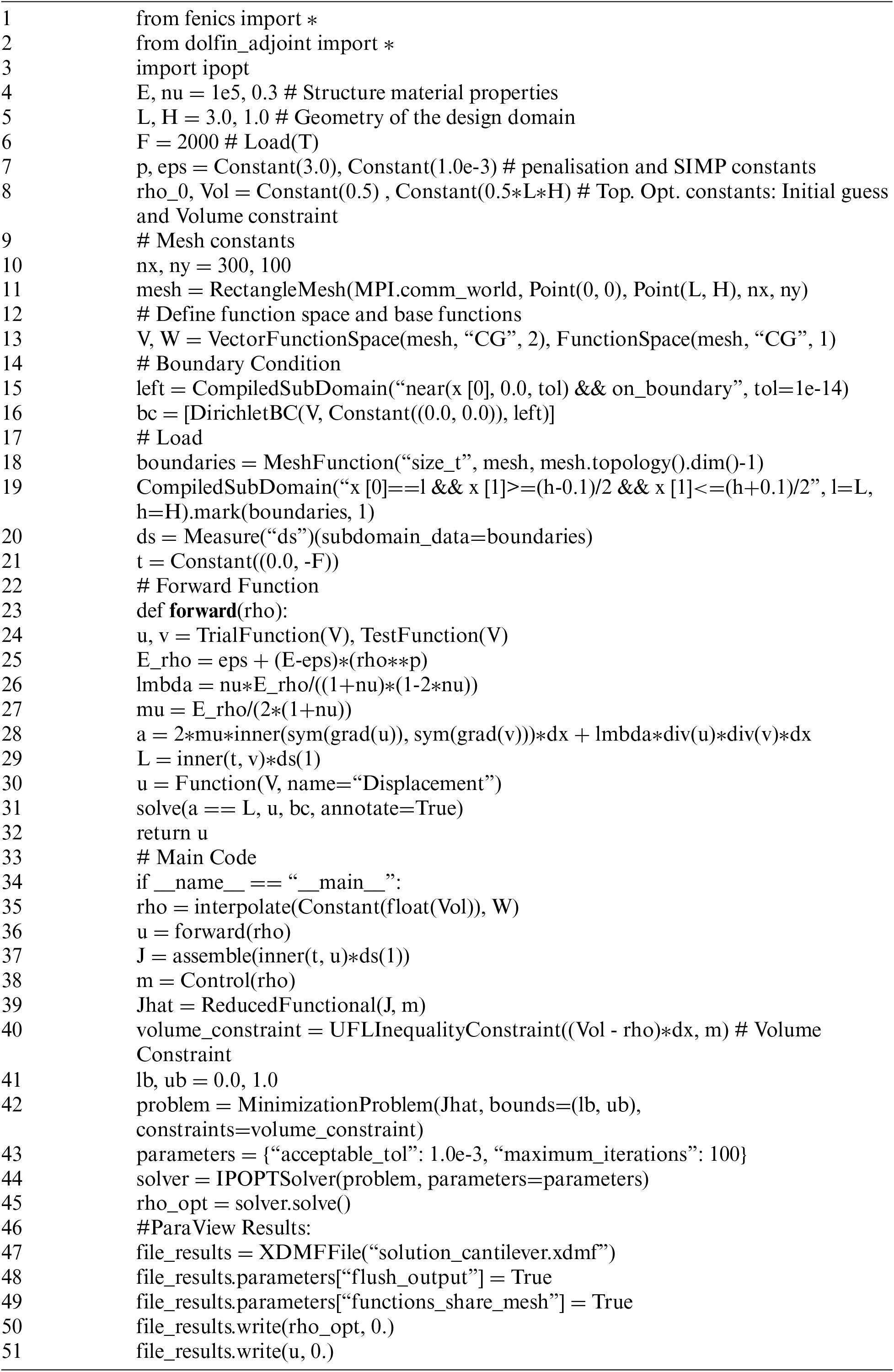
According to Code 1, first the FEniCS modules, Dolfin Adjoint and Ipopt are imported, lines 1 to 3 of the code.

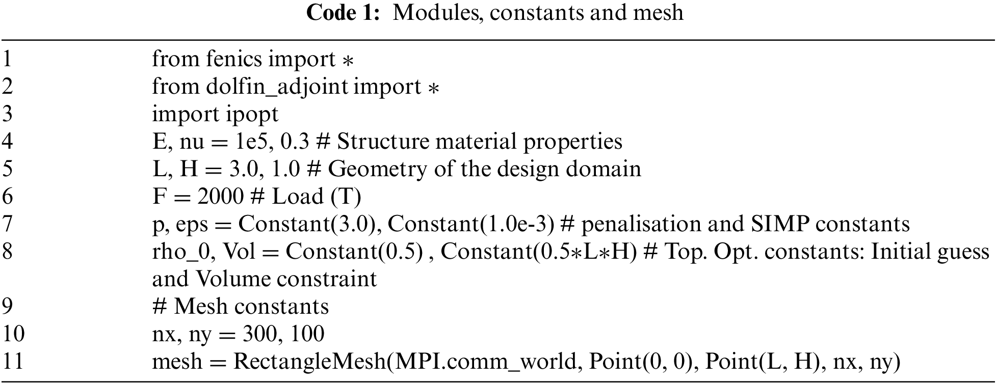
Then the material properties, geometry, loads, and topology optimization constants are defined on lines 4 to 8 of the code. And it follows defining the mesh declaration, lines 9 to 11. A rectangular mesh with width L and height H is declared with nx and ny divisions in the mesh in the horizontal and vertical directions, respectively. The last term of line 11 refers to the type of mesh, being optional; it indicates the direction of the diagonals and can be defined as “left”, “right”, “right/left”, “left/right” or “crossed”. See two mesh examples in Fig. 5 using linear triangles elements, by default.

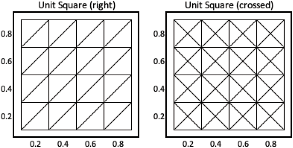
Figure 5: Example of mesh

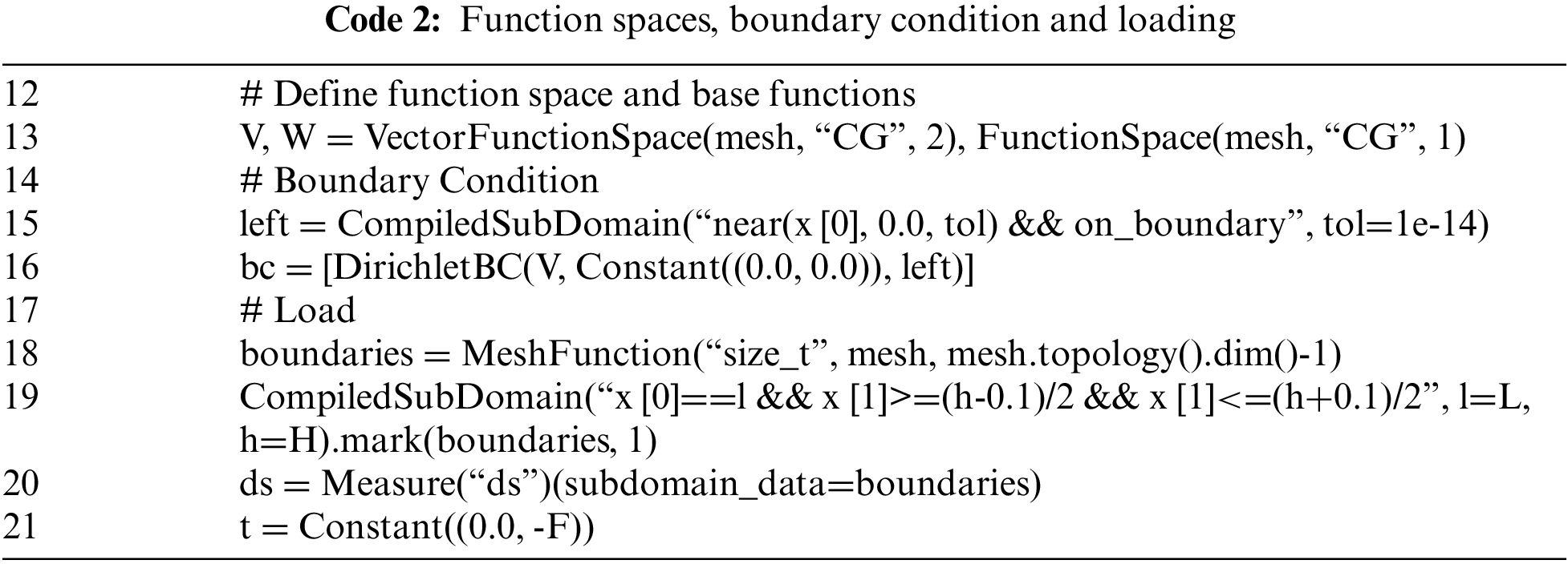
Continuing, according to Code 2, it is necessary to define the function spaces for the problem. For this, it is necessary to declare the mesh, the family of functions and the degree of the functions. It is used for the displacement, of the vector function space V, and the discretization made by functions of Continuous Galerkin, or “CG”, of degree 2. The degree is applied according to the number of divisions of each element. For the densities, the function space W is used and discretized by Galerkin Continuous functions of degree 1, lines 12 and 13 of the code.

See Fig. 6 for examples of linear Lagrange triangle element type for filtering and displacement, respectively.

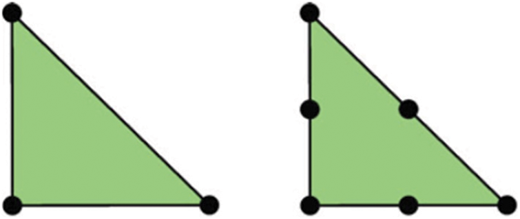
Figure 6: The linear Lagrange triangle: Filtering (“CG” 1) and Displacement (“CG” 2)

The next step is to define the boundary conditions and load case. This procedure is normally done by FEniCS through subdomains (SubDomain) and with that, a function call from C++ code to Python is required for each node in the mesh, which increases the computational cost. Thus, as a way of improving performance, the CompiledSubDomain command is used directly, which assumes a condition in C++ syntax, and converts the expression into an efficient compiled C++ function, significantly improving compilation time. For a cantilever beam fixed at the left end, the support is defined according to lines 14 to 16. The Dirichlet boundary condition, lines 17 to 21, is defined by assigning a zero value to the components of the displacement vector over the vector function space V. A concentrated load is inserted in the middle of the right side edge, which is also done using a CompiledSubDomain. In this case, it is necessary to use the discrete function, MeshFunction, which can be evaluated on the entities of a mesh. And according to the UFL (Unified Form Language) notation, ds denote the differential element for integration over the domain boundary. And used later, dx denotes the differential element for integration over the domain.

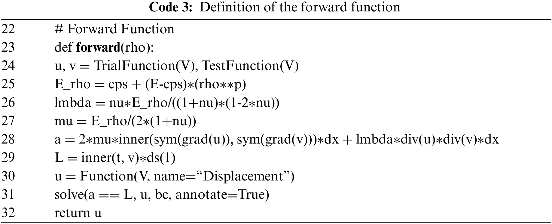
Now the solution to the Forward problem is defined and as a result obtaining the displacement variable, see Code 3, line 32. First, the functions trial and test are defined at line 24. Then, the SIMP interpolation of the modulus of elasticity seen in Eq. (15) is calculated in line 25, and its value is used to calculate the Lamé parameters and . Thus, the definition of the static equilibrium in the elastic variational form according to Eq. (13) is inserted in lines 28 and 29. Finally, all the parameters of the FEM are assembled, such as the matrix assemblies and the solution of the linear system through the solve function in line 31.

Thus, the code for the solution of the optimization problem, Code 4, is made. To solve the Forward problem, first the declaration of the initial density estimate is made through an interpolation, line 35, then in line 36, the Forward problem is called of Code 3 for this first estimate, and with that, FEniCS will solve the Forward problem at each iteration performing in the assembly process according to line 37. Continuing, Dolfin Adjoint continues the functional assembly process using the internal function ReducedFunctional, line 39, which solves the Forward problem using Dolfin Adjoint each time the functional is to be evaluated, and thus derives and solves the adjoint equation each time the functional gradient is to be evaluated, thereby generating the negative output of the displacement, that is, the maximization of the output displacement.

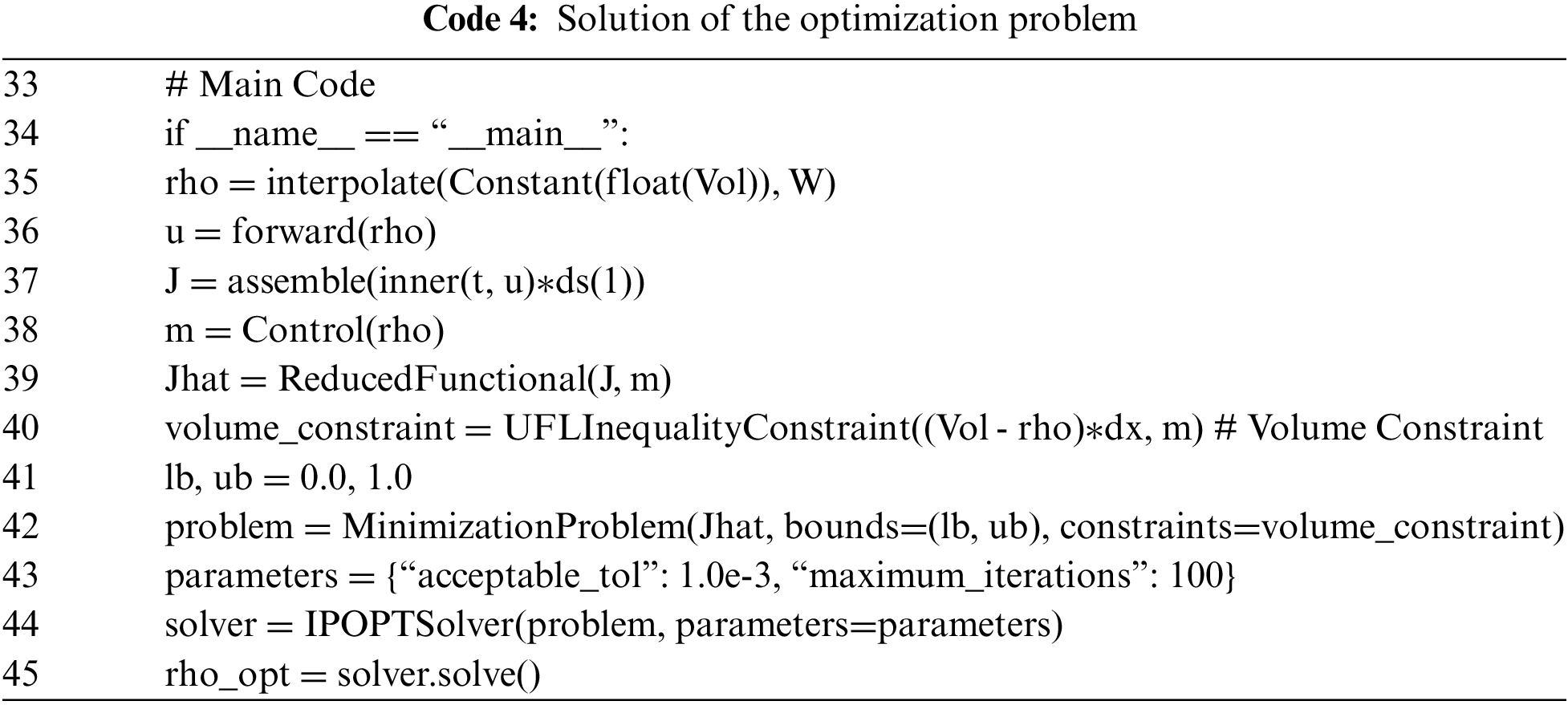
Next, the volume constraint must be defined according to Eq. (8). According to [75], the volume constraint must be calculated through the Jacobian according to Eqs. (18), (19). The constraint is implemented by the Dolfin Adjoint subclass UFLinequalityConstraint, according to line 40. In the present work, the volume constraint is 50% in relation to the original domain.

g(ρ)=V∗−∫Ωρ(x)dΩ=V∗−∫Ωρiϕi(x)dΩ(18)

∂g∂p=−∫Ωϕ1(x)dΩ⋮∫ΩϕM(x)dΩ(19)

Finally, the optimization problem is solved with the Minimization Problem function, line 42. The density constraint limits are inserted at line 41. The acceptance parameters and number of iterations, line 43, and with that they are released to the Ipopt solver, lines 44 and 45, ending the solution.

To visualize the solution, a Code 5 is generated, lines 46 to 51, used in the export to Paraview [76], which is an open-source cross-platform data visualization and analysis application.

The complete code is shown in Appendix A. The code produces the result shown in Fig. 7.

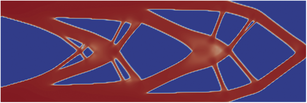
Figure 7: Optimization of a cantilever beam

4.1 Density Filter Implementation

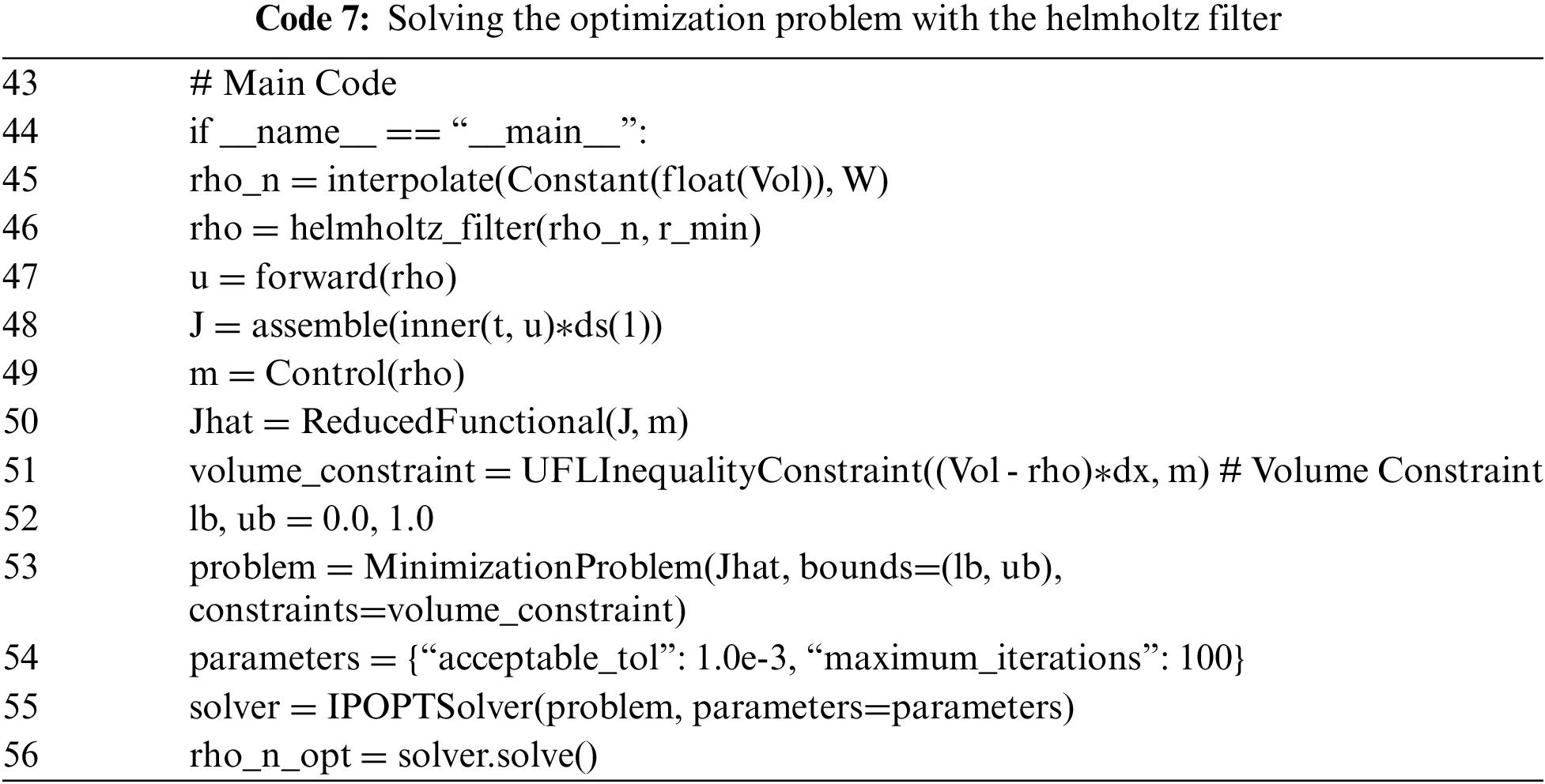
To improve the results as described in item 3 and according to Eq. (16), a mesh-dependent filter or density filter is inserted that can be implicitly represented by the solution of a partial differential equation of the Helmholtz type with Neumann homogeneous boundary conditions. Code 6 shows the application of the filter, and in Code 7 the solution call is reviewed, where it is necessary to perform the filter call within the main code, thus increasing the code by 11 lines only.

Running the code with the filter produces the result shown in Fig. 8.

Figure 8: Optimization of a Cantilever beam with the application of the density filter

The difference in the final result is clear when compared to the optimization of the same domain under different filtering conditions. The final distribution seen in Fig. 8 is structurally superior when compared to the final distribution seen in Fig. 7, where the final compliance for the unfiltered example is 3.21, and for the filtered example is 2.87. This shows the relevance of applying this type of filter. Finally, and perhaps most importantly, having both models with the same number of degrees of freedom at 241,602, the processing time for the unfiltered model was 393 seconds and the time for the filtered model was 334 seconds, or that is, demonstrating the prediction of improvement in processing time with the application of a Helmholtz-type density filter. For processing, a personal computer with a 3.6 GHz processor, Intel Core I9, 10-Core and 128 GB of memory was used.

5  Numerical Examples

5.1 MBB Beam (Messerschmitt-Bolkow-Blohm Beam)

The MBB beam is a classic problem in topology optimization. The design domain, the boundary conditions, and the external load for the MBB beam are shown in Fig. 9. Basically, what changes are the boundary conditions considering the support at the lower right end and the central region considering the symmetry of the domain and also the point of application of the load. This procedure is done through two subdomains, where the first subdomain is defined as class SimDB1(SubDomain) and the second subdomain is defined as class SimDB2 (SubDomain) completing the symmetry procedure. Code 8 shows the application of MMB beam.

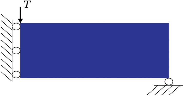
Figure 9: MBB beam

A concentrated load is applied to the upper left end, is considered, according to the same procedure as for the cantilever beam, inserting a subdomain defined as class LoadSurface (SubDomain). Running the code for the MBB beam example produces the result shown in Fig. 10.

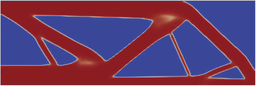
Figure 10: Optimization of an MBB beam

5.2 Multiple Loads

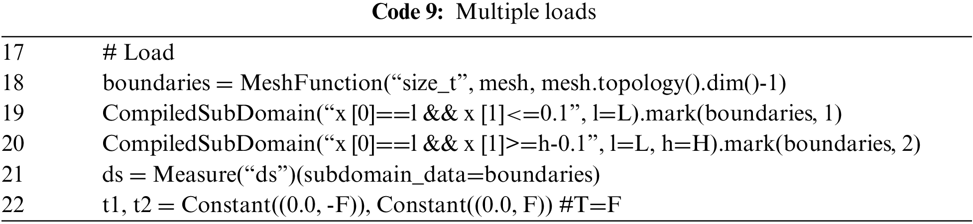
Extending the code base of a cantilever beam or any other model for any case considering multiple applied loads is also relatively simple. As shown in Fig. 11, an example where two loads are applied at the right end, both on the top edge and on the bottom edge.

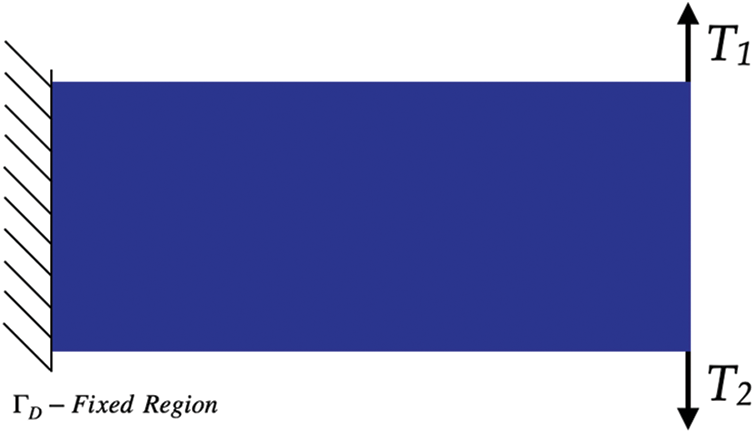
Figure 11: Cantilever beam with multiple loads

For this process, changing the load conditions for multiple loads is according to Code 9.

The difference now is that according to the equilibrium equations, the system is solved for each load. Thus, the functional becomes the sum of two Forward functions as seen in lines 46 and 47 of the revised main code as per Code 10.

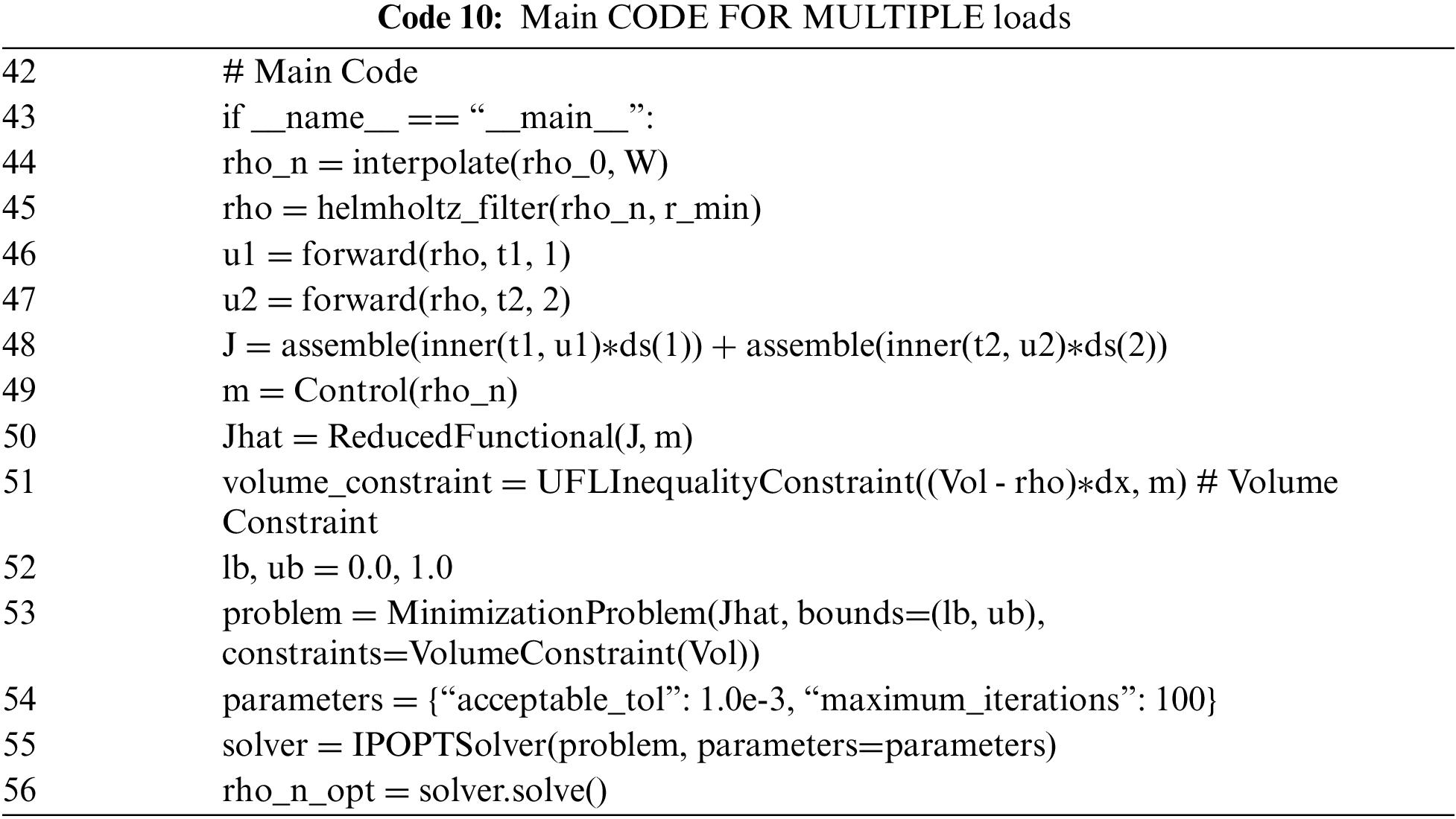
The optimized final result follows in Fig. 12.

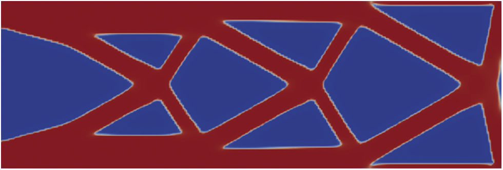
Figure 12: Optimization of a cantilever beam with multiple loads

According to Fig. 12, the result shows the similarity in the article by [3] of the “reinforcement” in the region of loads.

5.3 3D Cantilever

Making the switch from analyzing two-dimensional, or 2D, models to three-dimensional, or 3D models, is relatively easy using FEniCS. A change in the generation of the mesh and another in the application of the load, according to Code 11, are enough to solve the problem. In the 3D case, the geometric modification is for the length with L = 3.0, the height with H = 1 and the width with B = 0.2. The mesh divisions are 300, 100 and 20 in length, height and width, respectively. The other data and characteristics follow the same as the 2D model.

FEniCS developers have not updated the mesh generator for some time, which directly impacts optimization models that use the Dolfin Adjoint software, especially where mesh refinement or complex meshes are used. The justification is due to the existence of excellent external mesh generators that are compatible with FEniCS, which is the case of Gmsh [77], an open-source 3D finite element mesh generator with an integrated CAD engine and post-processor. The use of a structured and specific mesh generates an extra computational gain and is used in the 3D model in the present work. After generating the model in the Gmsh environment, a model conversion is first necessary so that FEniCS can process the model. This is done using the conversion package, meshio [78], and is done according to Code 12, which is independent of the solutions code.

After the conversion is done, it is necessary to call the 3D model by inserting Code 13 into the main code. The code is increased according to the project's needs and how the boundary and loading conditions will be used, and can be changed by some physical entity such as a line, face or volume.

The optimized final result follows in Fig. 13. The 3D model of a cantilever beam was made with a mesh of 333,453 elements and 1,454,448 degrees of freedom. Run time was approximately 7 h.

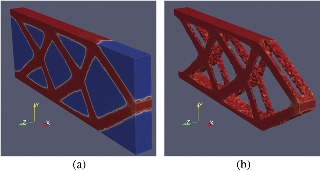
Figure 13: Optimization of a 3D cantilever beam. (a) showing the entire domain. (b) showing minimal topology

6  Parallelization with FEniCS and Dolfin Adjoint

Equations with the growing demand for new structural elements and the availability of advanced technological resources, numerical parallelization is increasingly evident. However, applying algorithmic differentiation to some codes that make use of parallelism is still a great challenge. Numerical algorithmic differentiation tools must be modified to meet the procedures of languages such as MPI (Message Passing Interface) and OpenMP and translate them into their parallel equivalents. So, for software like FEniCS and Dolfin Adjoint that makes use of high-level abstraction, the problem of parallelism disappears. With that, there is no specific code in Dolfin Adjoint to handle parallelism, deriving the adjoint at the right level of abstraction, the problem no longer exists. If the forward model runs in parallel, the adjoint model also runs in parallel, without modification. According to [79], Dolfin Adjoint handles parallel communication patterns automatically, even in the adjoint case. The high-level input in Dolfin Adjoint does not contain parallel communication calls, thus deriving the correct communication patterns at runtime.

The parallel communication patterns required for the adjoint equations are therefore automatically derived in exactly the same way as the parallel communication patterns for the forward equations, for both MPI and OpenMP cases. Direct implementation of the parallel adjoint model is a big advantage of adopting the combination of a high-level finite element system and a high-level approach to deriving its adjoint. So, to run all the examples of this work, the call in the terminal follows the following showing in Code 14.

7  Topology Evaluation by Iteration

An interesting aspect seen in many works on structural topology optimization is the visualization of the topology geometric evolution of the considered models, where it is possible to visualize the density of the model in each iteration, until the final convergence. Another important feature is the evaluation of the objective function, or in this case, Compliance as a function of the iteration compared to the reduction of the structure volume. These two evaluations are performed with a few lines of code by Dolfin Adjoint, according to Code 15. For this, Dolfin Adjoint creates a “tape” of the Forward model and sends it to the optimization process, repeatedly solving the Forward model and the adjoint model. With this it is possible to create a Callback for each iteration, where each Callback will produce a visualization format, VTK, possible to see in Paraview.

An evaluation of the evolution of Compliance and Volume Reduction by iteration is shown in Fig. 14.

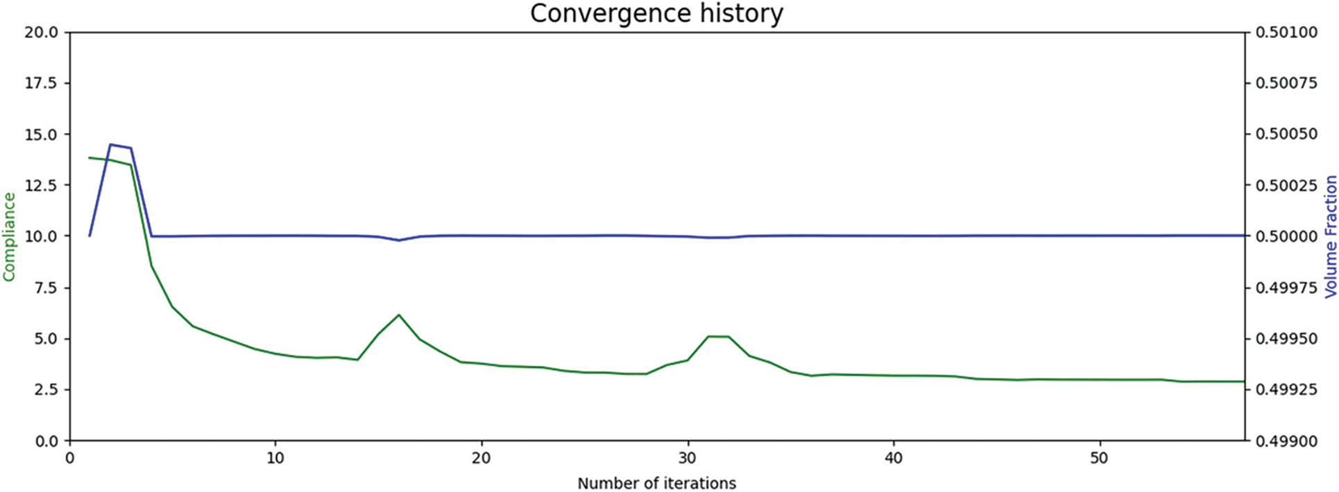
Figure 14: Compliance/Volume Fraction curve versus iteration

Below, in Fig. 15, are examples of iterations 01, 07, 13, 21, 31 and 45 of the cantilever model with density filter seen in Fig. 8.

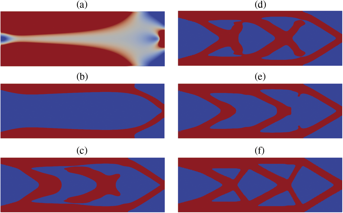
Figure 15: (a) Iteration 01, (b) Iteration 07, (c) Iteration 13, (d) Iteration 21, (e) Iteration 31 and (f) Iteration 45

8  Conclusions

This work demonstrated the application of a new open-source code for structural topology optimization with only 51 lines of code using open-source software for all stages of the topology optimization problem: modeling, sensitivity analysis, and optimization solver, totally open source and no other commercial software is required. It was shown that the application of the finite element method within its variational form with the use of its more abstract form follows an easy and intuitive pattern within the high-level possibilities treated by both FEniCS and Dolfin Adjoint.

Through the process of penalization by isotropic solid material, SIMP, it was possible to use the adjoint method to calculate the sensitivities considering the derivation of the functionals and later the optimization of the results by maximizing the displacements, or minimizing the compliance, using the package Ipopt which is also open-source and interacts with Dolfin Adjoint. The mesh generation is done for the most basic models within FEniCS itself or for more advanced projects with more geometric details, mainly models in three dimensions, done by the Gmsh software. The results of model visualization and image generation are done by the Paraview software, and thus, closing an entire process developed with open tools.

When comparing the results made here with already renowned works such as those seen in [3] that use the commercial MATLAB package or even more recent works, such as the one that also uses FEniCS itself in [25], we see that the results are very close, showing the viability of the codes generated here. The structural topology optimization of classic examples such as a cantilever beam with 60,000 elements made in a few minutes shows the high-performance capability of the open-source package. And even though they are free, FEniCS and Dolfin Adjoint have a very active community and researchers from numerous institutions using and enabling the exchange of information and support for research.

Thus, the present work shows that it is possible to use open tools in structural topology optimization projects, being possible to replicate by the academic community in general without the need for software acquisition costs for their projects.

Acknowledgement: Thanks to IFES-Federal Institute of Espírito Santo for the encouragement and availability to provide the opportunity for Dinter-Interinstitutional Doctorate with Unicamp-State University of Campinas. Thank CAPES-Coordination for the Improvement of Higher Education Personnel for the scholarships made available during part of the research period.

Funding Statement: The authors would like to thank the Faculty of Mechanical Engineering at Unicamp and CAPES for financial support for this article.

Conflicts of Interest: The authors declare that they have no conflicts of interest to report regarding the present study.

Appendix A

References

1. Bendsoe, M. P., Sigmund, O. (2003). Topology optimization: Theory, methods, and applications. Berlin Heidelberg: Springer. 10.1007/978-3-662-05086-6 [Google Scholar] [CrossRef]
2. Dorn, W., Gomory, R., Greenberg, H. J. (1964). Automatic design of optimal structures, computer science. Journal de Mecanique, 3, 25–52. [Google Scholar]
3. Aranda, E., Bellido, J. C. (2016). Introduction to truss structures optimization with python. Electronic Journal of Mathematics and Technology, 10(1), GALEA673737392. [Google Scholar]
4. Goldberg, D. E. (1989). Genetic algorithms in search. In: Optimization, and machine learning. Addison-Wesley. [Google Scholar]
5. Bonyadi, M. R., Michalewicz, Z. (2017). Particle swarm optimization for single objective continuous space problems: A review. Evolutionary Computation, 25(1), 1–54. DOI 10.1162/EVCO_r_00180. [Google Scholar] [CrossRef]
6. Dorigo, M., Maniezzo, V., Colorni, A. (1996). Ant system: Optimization by a colony of cooperating agents. IEEE Transactions on Systems, Man, and Cybernetics, Part B (Cybernetics), 26(1), 29–41. DOI 10.1109/3477.484436. [Google Scholar] [CrossRef]
7. Xie, Y. M., Steven, G. P. (1993). A simple evolutionary procedure for structural optimization. Computers and Structures, 49(3), 885–896. DOI 10.1016/0045-7949(93)90035-C. [Google Scholar] [CrossRef]
8. Picelli, R., Sivapuram, R., Xie, Y. M. (2021). A 101-line MATLAB code for topology optimization using binary variables and integer programming. Structural and Multidisciplinary Optimization, 63(2), 935–954. DOI 10.1007/s00158-020-02719-9. [Google Scholar] [CrossRef]
9. Bendsøe, M. P., Kikuchi, N. (1988). Generating optimal topologies in structural design using a homogenization method. Computer Methods in Applied Mechanics and Engineering, 71(2), 197–224. DOI 10.1016/0045-7825(88)90086-2. [Google Scholar] [CrossRef]
10. Bendsøe, M. P., Ben-Tal, A., Zowe, J. (1994). Optimization methods for truss geometry and topology design. Structural Optimization, 7(3), 141–159. DOI 10.1007/BF01742459. [Google Scholar] [CrossRef]
11. Kirsch, U. (1989). Optimal topologies of structures. Applied Mechanics Reviews, 42(8), 223–239. DOI 10.1115/1.3152429. [Google Scholar] [CrossRef]
12. Rozvany, G. I. N., Bendsø, M. P., Kirsch, U. (1995). Layout optimization of structures. Applied Mechanics Reviews, 48(2), 41–119. DOI 10.1115/1.3005097. [Google Scholar] [CrossRef]
13. Lee, E. H., Park, J. (2011). Structural design using topology and shape optimization. Structural Engineering and Mechanics, 38(4), 517–527. DOI 10.12989/sem.2011.38.4.517. [Google Scholar] [CrossRef]
14. Gil, L., Andreu, A. (2001). Shape and cross-section optimization of a truss structure. Computers and Structures, 79(7), 681–689. DOI 10.1016/S0045-7949(00)00182-6. [Google Scholar] [CrossRef]
15. Reddy, G. M., Cagan, J. (1995). Optimally directed truss topology generation using shape annealing. Journal of Mechanical Design, Transactions of the ASME, 117(1), 206–209. DOI 10.1115/1.2826110. [Google Scholar] [CrossRef]
16. Shea, K., Cagan, J., Fenves, S. J. (1997). A shape annealing approach to optimal truss design with dynamic grouping of members. Journal of Mechanical Design, 119(3), 388–394. DOI 10.1115/1.2826360. [Google Scholar] [CrossRef]
17. Suzuki, K., Kikuchi, N. (1991). A homogenization method for shape and topology optimization. Computer Methods in Applied Mechanics and Engineering, 93(3), 291–318. DOI 10.1016/0045-7825(91)90245-2. [Google Scholar] [CrossRef]
18. Díaaz, A. R., Kikuchi, N. (1992). Solutions to shape and topology eigenvalue optimization problems using a homogenization method. International Journal for Numerical Methods in Engineering, 35(7), 1487–1502. DOI 10.1002/(ISSN)1097-0207. [Google Scholar] [CrossRef]
19. Ma, Z. D., Kikuchi, N., Cheng, H. C. (1995). Topology design for vibrating structures. Computer Methods in Applied Mechanics and Engineering, 121(1–4), 259–280. DOI 10.1016/0045-7825(94)00714-X. [Google Scholar] [CrossRef]
20. Teimouri, M., Asgari, M. (2019). Multi-objective BESO topology optimization for stiffness and frequency of continuum structures. Structural Engineering and Mechanics, 72(2), 181–190. DOI 10.12989/SEM.2019.72.2.181. [Google Scholar] [CrossRef]
21. Luo, J., Gea, H. C., Yang, R. J. (2000). Topology optimization for crush design. 8th Symposium on Multidisciplinary Analysis and Optimization, Long Beach, CA, U.S.A. DOI 10.2514/6.2000-4770. [Google Scholar] [CrossRef]
22. Li, H., Wang, D., Zhang, H., Wang, X., Qin, Z. et al. (2022). Optimal design of vibro-impact resistant fiber reinforced composite plates with polyurea coating. Composite Structures, 292(12), 115680. DOI 10.1016/j.compstruct.2022.115680. [Google Scholar] [CrossRef]
23. Sato, Y., Izui, K., Yamada, T., Nishiwaki, S., Ito, M. et al. (2019). Reliability-based topology optimization under shape uncertainty modeled in Eulerian description. Structural and Multidisciplinary Optimization, 59(1), 75–91. DOI 10.1007/s00158-018-2051-y. [Google Scholar] [CrossRef]
24. Sigmund, O. (2001). A 99 line topology optimization code written in Matlab. Structural and Multidisciplinary Optimization, 21(2), 120–127. DOI 10.1007/s001580050176. [Google Scholar] [CrossRef]
25. Huang, X., Xie, Y. M. (2010a). A further review of ESO type methods for topology optimization. Structural and Multidisciplinary Optimization, 41(5), 671–683. DOI 10.1007/s00158-010-0487-9. [Google Scholar] [CrossRef]
26. Huang, X., Xie, Y. M. (2010b). Evolutionary topology optimization of continuum structures: Methods and applications. UK: John Wiley & Sons. DOI 10.1002/9780470689486 [Google Scholar] [CrossRef]
27. Rong, J. H., Xie, Y. M., Yang, X. Y., Linag, Q. Q. (2000). Topology optimization of structures under dynamic response constraints. Journal of Sound and Vibration, 234(2), 177–189. DOI 10.1006/jsvi.1999.2874. [Google Scholar] [CrossRef]
28. Xie, Y. M., Steven, G. P. (1996). Evolutionary structural optimization for dynamic problems. Computers and Structures, 58(6), 1067–1073. DOI 10.1016/0045-7949(95)00235-9. [Google Scholar] [CrossRef]
29. Xie, Y. M., Steven, G. P. (1997). Basic evolutionary structural optimization. In: Evolutionary structural optimization. London: Springer. DOI 10.1007/978-1-4471-0985-3_2. [Google Scholar] [CrossRef]
30. Yang, X. Y., Xie, Y. M., Steven, G. P., Querin, O. M. (1999). Bidirectional evolutionary method for stiffness optimization. AIAA Journal, 37(11), 1483–1488. DOI 10.2514/2.626. [Google Scholar] [CrossRef]
31. Zhu, R., Zhang, X., Zhang, S., Dai, Q., Qin, Z. et al. (2022). Modeling and topology optimization of cylindrical shells with partial CLD treatment. International Journal of Mechanical Sciences, 220(2), 107145. DOI 10.1016/j.ijmecsci.2022.107145. [Google Scholar] [CrossRef]
32. Allaire, G., Jouve, F., Toader, A. M. (2004). Structural optimization using sensitivity analysis and a level-set method. Journal of Computational Physics, 194(1), 363–393. DOI 10.1016/j.jcp.2003.09.032. [Google Scholar] [CrossRef]
33. Shu, L., Wang, M. Y., Fang, Z., Ma, Z., Wei, P. (2011). Level set based structural topology optimization for minimizing frequency response. Journal of Sound and Vibration, 330(24), 5820–5834. DOI 10.1016/j.jsv.2011.07.026. [Google Scholar] [CrossRef]
34. Wang, M. Y., Wang, X., Guo, D. (2003). A level set method for structural topology optimization. Computer Methods in Applied Mechanics and Engineering, 192(1–2), 227–246. DOI 10.1016/S0045-7825(02)00559-5. [Google Scholar] [CrossRef]
35. Guo, X., Zhang, W. S., Zhang, J., Yuan, J. (2016). Explicit structural topology optimization based on moving morphable components (MMC) with curved skeletons. Computer Methods in Applied Mechanics and Engineering, 310, 711–748. DOI 10.1016/j.cma.2016.07.018. [Google Scholar] [CrossRef]
36. Wang, R., Zhang, X., Zhu, B. (2019). Imposing minimum length scale in moving morphable component (MMC)-based topology optimization using an effective connection status (ECS) control method. Computer Methods in Applied Mechanics and Engineering, 351(2), 667–693. DOI 10.1016/j.cma.2019.04.007. [Google Scholar] [CrossRef]
37. Challis, V. J. (2010). A discrete level-set topology optimization code written in Matlab. Structural and Multidisciplinary Optimization, 41(3), 453–464. DOI 10.1007/s00158-009-0430-0. [Google Scholar] [CrossRef]
38. Andreassen, E., Clausen, A., Schevenels, M., Lazarov, B. S., Sigmund, O. (2011). Efficient topology optimization in MATLAB using 88 lines of code. Structural and Multidisciplinary Optimization, 43(1), 1–16. DOI 10.1007/s00158-010-0594-7. [Google Scholar] [CrossRef]
39. Talischi, C., Paulino, G. H., Pereira, A., Menezes, I. F. M. (2012). PolyTop: A matlab implementation of a general topology optimization framework using unstructured polygonal finite element meshes. Structural and Multidisciplinary Optimization, 45(3), 329–357. DOI 10.1007/s00158-011-0696-x. [Google Scholar] [CrossRef]
40. Liu, K., Tovar, A. (2014). An efficient 3D topology optimization code written in matlab. Structural and Multidisciplinary Optimization, 50(6), 1175–1196. DOI 10.1007/s00158-014-1107-x. [Google Scholar] [CrossRef]
41. Tavakoli, R., Mohseni, S. M. (2014). Alternating active-phase algorithm for multimaterial topology optimization problems: A 115-line MATLAB implementation. Structural and Multidisciplinary Optimization, 49(4), 621–642. DOI 10.1007/s00158-013-0999-1. [Google Scholar] [CrossRef]
42. Zuo, Z. H., Xie, Y. M. (2015). A simple and compact Python code for complex 3D topology optimization. Advances in Engineering Software, 85(1), 1–11. DOI 10.1016/j.advengsoft.2015.02.006. [Google Scholar] [CrossRef]
43. Xia, L., Breitkopf, P. (2015). Design of materials using topology optimization and energy-based homogenization approach in matlab. Structural and Multidisciplinary Optimization, 52(6), 1229–1241. DOI 10.1007/s00158-015-1294-0. [Google Scholar] [CrossRef]
44. Zhang, W., Yuan, J., Zhang, J., Guy, X. (2016). A new topology optimization approach based on Moving Morphable Components (MMC) and the ersatz material model. Structural and Multidisciplinary Optimization, 53(6), 1243–1260. DOI 10.1007/s00158-015-1372-3. [Google Scholar] [CrossRef]
45. Ansola Loyola, R., Querin, O. M., Garaigordobil Jiménez, A., Alonso Gordoa, C. (2018). A sequential element rejection and admission (SERA) topology optimization code written in Matlab. Structural and Multidisciplinary Optimization, 58(3), 1297–1310. DOI 10.1007/s00158-018-1939-x. [Google Scholar] [CrossRef]
46. Wei, P., Li, Z., Li, X., Wang, M. Y. (2018). An 88-line MATLAB code for the parameterized level set method based topology optimization using radial basis functions. Structural and Multidisciplinary Optimization, 58(2), 831–849. DOI 10.1007/s00158-018-1904-8. [Google Scholar] [CrossRef]
47. Xia, L., Xia, Q., Huang, X., Huang, X., Xie, Y. M. (2018). Bi-directional evolutionary structural optimization on advanced structures and materials: A comprehensive review. Archives of Computational Methods in Engineering, 25(2), 437–478. DOI 10.1007/s11831-016-9203-2. [Google Scholar] [CrossRef]
48. Laurain, A. (2018). A level set-based structural optimization code using FEniCS. Structural and Multidisciplinary Optimization, 58(3), 1311–1334. DOI 10.1007/s00158-018-1950-2. [Google Scholar] [CrossRef]
49. Chen, Q., Zhang, X., Zhu, B. (2019). A 213-line topology optimization code for geometrically nonlinear structures. Structural and Multidisciplinary Optimization, 59(5), 1863–1879. DOI 10.1007/s00158-018-2138-5. [Google Scholar] [CrossRef]
50. Lagaros, N. D., Vasileiou, N., Kazakis, G. A. (2019). C# code for solving 3D topology optimization problems using SAP2000. Optimization and Engineering, 20(1), 1–35. DOI 10.1007/s11081-018-9384-7. [Google Scholar] [CrossRef]
51. Liang, Y., Cheng, G. (2020). Further elaborations on topology optimization via sequential integer programming and Canonical relaxation algorithm and 128-line MATLAB code. Structural and Multidisciplinary Optimization, 61(1), 411–431. DOI 10.1007/s00158-019-02396-3. [Google Scholar] [CrossRef]
52. Kim, C., Jung, M., Yamada, T., Nishiwaki, S., Yoo, J. (2020). FreeFEM++ code for reaction-diffusion equation-based topology optimization: For high-resolution boundary representation using adaptive mesh refinement. Structural and Multidisciplinary Optimization, 62(1), 439–455. DOI 10.1007/s00158-020-02498-3. [Google Scholar] [CrossRef]
53. Yaghmaei, M., Ghoddosian, A., Khatibi, M. M. (2020). A filter-based level set topology optimization method using a 62-line MATLAB code. Structural and Multidisciplinary Optimization, 62(2), 1001–1018. DOI 10.1007/s00158-020-02540-4. [Google Scholar] [CrossRef]
54. Ferrari, F., Sigmund, O. (2020). A new generation 99 line matlab code for compliance topology optimization and its extension to 3D. Structural and Multidisciplinary Optimization, 62(4), 2211–2228. DOI 10.1007/s00158-020-02629-w. [Google Scholar] [CrossRef]
55. Gupta, A., Chowdhury, R., Chakrabarti, A., Rabczuk, T. (2020). A 55-line code for large-scale parallel topology optimization in 2D and 3D. DOI 10.48550/arXiv.2012.0820. [Google Scholar] [CrossRef]
56. Zhu, B., Zhang, X., Li, H., Liang, J., Wang, R. et al. (2021). An 89-line code for geometrically nonlinear topology optimization written in FreeFEM. Structural and Multidisciplinary Optimization, 63(2), 1015–1027. DOI 10.1007/s00158-020-02733-x. [Google Scholar] [CrossRef]
57. Wang, C., Zhao, Z., Zhou, M., Sigmund, O., Zhang, X. S. (2021). A comprehensive review of educational articles on structural and multidisciplinary optimization. Structural and Multidisciplinary Optimization, 64(5), 2827–2880. DOI 10.1007/s00158-021-03050-7. [Google Scholar] [CrossRef]
58. Langtangen, H. P., Logg, A. (2016). Solving PDEs in python. Cham: Springer. DOI 10.1007/978-3-319-52462-7 [Google Scholar] [CrossRef]
59. Alnæs, M., Blechta, J., Hake, J., Johansson, A., Kehlet, B. et al. (2015). The FEniCS Project Version 1.5. Archive of Numerical Software:3. DOI 10.11588/ans.2015.100.20553. [Google Scholar] [CrossRef]
60. Logg, A., Wells, G., Mardal, K. A. (2011). Automated solution of differential equations by the finite element method, the FEniCS book. Berlin: Springer. arXiv:2001.10058. DOI 10.1007/978-3-642-23099-8 [Google Scholar] [CrossRef]
61. Dokken, J. S., Mitusch, S. K., Funke, S. W. (2020). Automatic shape derivatives for transient PDEs in FEniCS and Firedrake. DOI 10.48550/arXiv.2001.10058. [Google Scholar] [CrossRef]
62. Funke, S. W., Farrell, P. E. (2013). A framework for automated PDE-constrained optimisation. arXiv:2001.10058. DOI 10.48550/arXiv.1302.3894. [Google Scholar] [CrossRef]
63. Mitusch, S., Funke, S., Dokken, J. (2019). Dolfin-adjoint 2018.1: Automated adjoints for FEniCS and Firedrake. Journal of Open Source Software, 4(38). DOI 10.21105/joss.01292. [Google Scholar] [CrossRef]
64. Bendsøe, M., Sigmund, O. (1999). Material interpolation schemes in topology optimization. Archive of Applied Mechanics, 69(9–10), 635–654. DOI 10.1007/s004190050248. [Google Scholar] [CrossRef]
65. Tcherniak, D. (2002). Topology optimization of resonating structures using SIMP method. International Journal for Numerical Methods in Engineering, 54(11), 1605–1622. DOI 10.1002/(ISSN)1097-0207. [Google Scholar] [CrossRef]
66. Naumann, U. (2011). The art of differentiating computer programs. In: Society for industrial and applied mathematics. Philadelphia, USA. [Google Scholar]
67. Langtangen, H. P., Mardal, K. A. (2019). Introduction to numerical methods for variational problems. Cham: Springer. DOI 10.1007/978-3-030-23788-2 [Google Scholar] [CrossRef]
68. Gockenbach, M. S. (2006). Understanding and implementing the finite element method. Society for Industrial and Applied Mathematics (SIAM). DOI 10.1137/1.9780898717846. [Google Scholar] [CrossRef]
69. Larson, M., Bengzon, F. (2013). The finite element method: Theory, implementation, and applications. Berlin, Heidelberg: Springer. DOI 10.1007/978-3-642-33287-6 [Google Scholar] [CrossRef]
70. Díaz, A., Sigmund, O. (1995). Checkerboard patterns in layout optimization. Structural Optimization, 10(1), 40–45. DOI 10.1007/BF01743693. [Google Scholar] [CrossRef]
71. Jog, C. S., Haber, R. B. (1996). Stability of finite element models for distributed-parameter optimization and topology design. Computer Methods in Applied Mechanics and Engineering, 130(3–4), 203–226. DOI 10.1016/0045-7825(95)00928-0. [Google Scholar] [CrossRef]
72. Sigmund, O., Petersson, J. (1998). Numerical instabilities in topology optimization: A survey on procedures dealing with checkerboards, mesh-dependencies and local minima. Structural Optimization, 16(1), 68–75. DOI 10.1007/BF01214002. [Google Scholar] [CrossRef]
73. Lazarov, B. S., Sigmund, O. (2011). Filters in topology optimization based on helmholtz-type differential equations. International Journal for Numerical Methods in Engineering, 86(6), 765–781. DOI 10.1002/nme.3072. [Google Scholar] [CrossRef]
74. Wächter, A., Biegler, L. (2006). On the implementation of an interior-point filter line-search algorithm for large-scale nonlinear programming. Mathematical Programming, 106(1), 25–57. DOI 10.1007/s10107-004-0559-y. [Google Scholar] [CrossRef]
75. Souza, E. (2020). Design of pneumatic and hydraulic soft actuators by topology optimization method (Dissertation). Brazil: USP. [Google Scholar]
76. Squillacote, A. H. (2007). The paraview guide. 3rd edition. ParaView: Kitware, Inc. [Google Scholar]
77. Remacle, J., Geuzaine, C. (2009). Gmsh: A 3-D finite element mesh generator with built-in pre- and post-processing. International Journal for Numerical Methods in Engineering, 79(11), 1309–1331. DOI 10.1002/nme.2579. [Google Scholar] [CrossRef]
78. Schlömer, N., Nilswagner, Li, T., Coutinho, T., Dalcin, C. et al. (2018). Nschloe/meshio v1.11.7 - I/O for various mesh formats. DOI 10.5281/zenodo.1173116. [Google Scholar] [CrossRef]
79. Farrell, P. E., Ham, D. A., Funke, S. W., Rognes, M. E. (2013). Automated derivation of the adjoint of high-level transient finite element programs. SIAM Journal on Scientific Computing, 35(4), C369–C393. DOI 10.1137/120873558. [Google Scholar] [CrossRef]
Appendix A
Cite This Article
Copyright © 2023 The Author(s). Published by Tech Science Press.
This work is licensed under a Creative Commons Attribution 4.0 International License , which permits unrestricted use, distribution, and reproduction in any medium, provided the original work is properly cited.
Downloads
Citation Tools