
 Submit a Paper
 Propose a Special lssue
 Open Access
ARTICLE

Numerical Simulation of Fretting Fatigue Damage Evolution of Cable Wires Considering Corrosion and Wear Effects
Key Laboratory of Concrete and Prestressed Concrete Structures of Ministry of Education, Southeast University, Nanjing, 211189, China
* Corresponding Author: Ying Wang. Email:
Computer Modeling in Engineering & Sciences 2023, 136(2), 1339-1370. https://doi.org/10.32604/cmes.2023.025830
Received 01 August 2022; Accepted 08 October 2022; Issue published 06 February 2023
 View Full Text
 Download PDF
Abstract
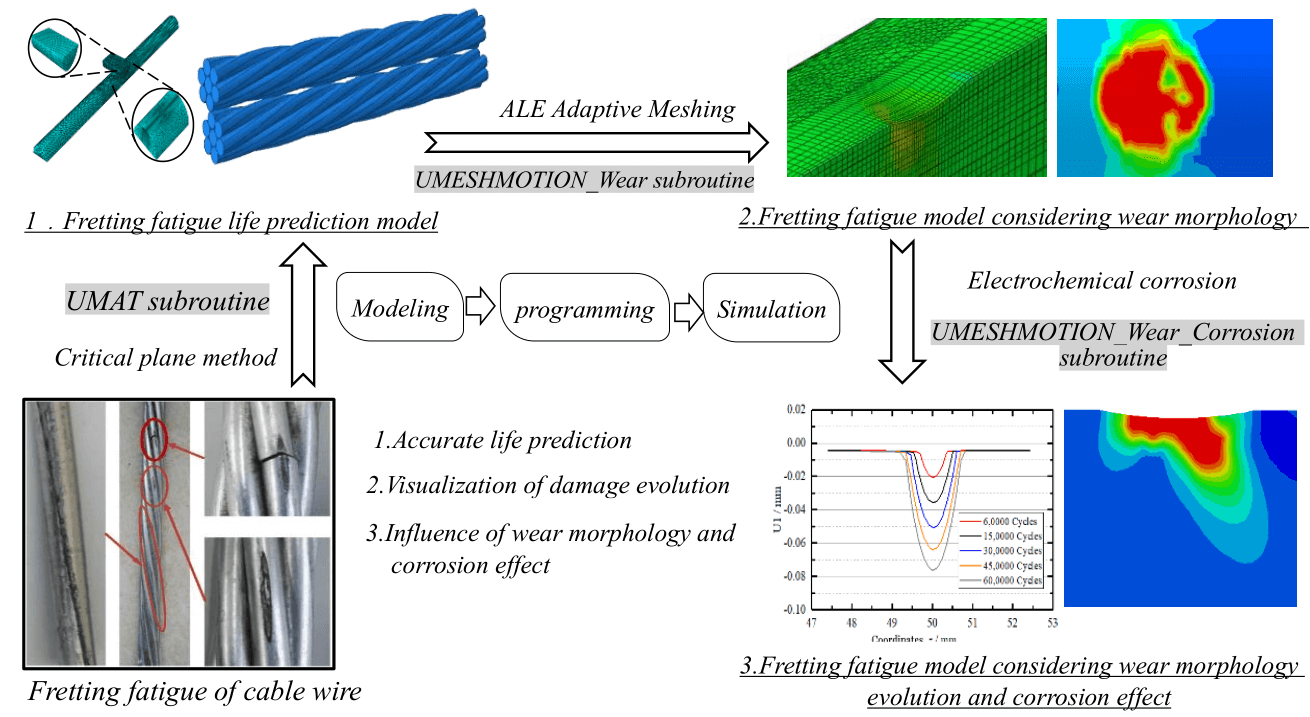
In this paper, a numerical model of fretting fatigue analysis of cable wire and the fretting fatigue damage constitutive model considering the multi-axis effect were established, and the user material subroutine UMAT was written. Then, the constitutive model of wear morphology evolution of cable wire and the constitutive model of pitting evolution considering the mechanical-electrochemical effect were established, respectively. The corresponding subroutines UMESHMOTION_Wear and UMESHMOTION_Wear_Corrosion were written, and the fretting fatigue life was further predicted. The results show that the numerical simulation life obtained by the program in this paper has the same trend as the tested one; the error is only about 0.7% in the medium life area; When the normal contact force increases from 120 to 240 N, the fretting life of cable wire decreases by 25%; When the evolution of wear morphology and corrosion effect are considered simultaneously, the depth of the wear zone exceeds 0.08 mm after 600,000 loads, which is much larger than 0.04 mm when only the evolution of wear morphology is considered. When the evolution of wear morphology and corrosion morphology is considered simultaneously, the damage covers the whole contact surface after 300,000 loads, and the penetrating damage zone forms after 450,000 loads, which is obviously faster than that when only the wear morphology evolution is considered. The method proposed in this paper can provide a feasible numerical simulation scheme for the visualization of the damage process and accurate life prediction of cable-supported bridges.Graphic Abstract
Keywords
Fretting refers to the extremely small relative motion of two contact surfaces, which usually consists in “the approximate fastening” mechanical components. Fretting fatigue refers to the mechanical behavior in which one of the two contact pairs frets under an external fatigue load. Wear is one of the results induced by fretting fatigue behavior between cables, which results in microstructure changes and local stress concentration of cables, and makes the actual life of cables much lower than the expected life.
Studies show that the alternating action of multiaxial stress is the main reason for the fatigue failure of fastening components [1]. However, existing studies often adopt the theoretical method of transforming the multiaxial stress state into the uniaxial stress state, which cannot reflect the real situation of damage and failure caused by multiaxial fatigue. The multiaxial fatigue theory based on the critical plane breaks through the deficiency of transforming the multiaxial stress state into the uniaxial stress state. The method was developed based on the observation of fatigue crack nucleation and cracking of metal materials with polycrystalline structures. The stress and strain parameters on the plane of maximum damage were used as multiaxial fatigue damage parameters, which reflected the physical significance of the existence of multiaxial failure plane. This method has been proven to have important engineering application value. However, due to the diversity of the forces on the research object, no model has universal applicability at present [2,3].
Under the action of dead weight and wind and rain excitation, the cable steel wire will produce repeated vibration and relative dislocation in the cable plane [4], which is consistent with fretting fatigue theory in mechanism. Therefore, it is reasonable to use fretting fatigue theory to analyze the fatigue problem of tight contact between wires in cables. At the same time, rain erosion, oxygen infiltration and other effects will lead to electrochemical corrosion behavior of cable wire. It has been proved in engineering practice that the corrosion fatigue failure of cable wire caused by fretting fatigue load and corrosive medium is one of its typical failure modes, and its essence is the coupling of mechanical and electrochemical processes. This process combines many factors, such as mechanical factors, environmental factors and materials. The combined action of mechanics and electrochemistry exceeds the simple superposition of alternating load and corrosive medium alone, resulting in the change of microstructure and local stress concentration of the cable wire, which makes its actual life much lower than the expected life.
Relevant studies show that corrosion pits are the main area of microcrack initiation, and loading can promote the formation of corrosion pits. When the depth of corrosion pits reaches 5 mm, the probability of crack initiation near corrosion pits is up to 90% [5]. Lan et al. [6] carried out hydrochloric acid accelerated corrosion tests on cable wires, fitted a multi-parameter fatigue life model of corroded steel wires from the test data, then the fatigue damage evolution model using multi-step load was used to predict the fatigue life. Li et al. [7] conducted fatigue tests on corroded steel wires and found that fatigue fracture forms were related to the degree of corrosion. Li et al. [8] simulated the corrosion behavior of steel strands in acid rain by soaking them in NaCl solution, and obtained the corrosion potential and corrosion rate of steel strands to obtain the parameters related to the deterioration of steel strands’ performance.
Wang et al. [9] studied the effect of the plastic zone at the crack tip on the crack propagation law using the extended finite element method. Then they improved the cellular automata corrosion model, and established a parameterized corrosion probability model of reinforcement in concrete based on the inhomogeneity of corrosion space, which realized the prediction and simulation of corrosion morphology [10]. Yu et al. [11] established the corrosion model of cable wire by using user-defined FORTRAN subroutine and realized random stress corrosion. The corrosion morphology and fracture strength of the wire rope with time change were obtained. Wang et al. [12] established a numerical model of mechano-electrochemical interaction, and studied the influence of single and two adjacent local corrosion defects on the burst strength of pipelines. Then they assessed the buckling behavior of axial compressed H-shape column with time-variant corrosion defects, based on the user-defined UMESHMOTION subroutine, the rules of corrosion morphology and collapse force of axial compression H-shape column changing with time are obtained [13]. Xu et al. [14] established a finite element model of pipeline corrosion defects growing with time, quantitatively analyzed the synergistic effect of stress and local corrosion reaction. These above literatures provide numerical models of component deterioration under stress-corrosion, but do not consider the influence of fretting fatigue and the wear morphology evolution caused by fretting fatigue.
In conclusion, the fracture failure of cable wire is a complex process caused by fretting fatigue and electrochemical corrosion coupling. Most of the existing studies use the experimental method to simplify the fatigue behavior of parallel wire bundles to the fatigue behavior of single wire, and the life prediction formula is fitted by the accelerated corrosion and fatigue test data. The obtained formula has poor applicability, the coupled damage theory that can be quantitatively analyzed has not been summarized, and the corresponding numerical simulation scheme of damage evolution is lacking. The multiaxial fatigue theory based on the critical plane theory provides the possibility to study the fretting fatigue life of cable wires, but some related numerical simulation work fails to consider the influence of complex three-dimensional problems and wear morphology evolution. Therefore, starting from the fretting fatigue mechanism of steel wire, this paper first established fretting fatigue damage constitutive model and corrosion pit evolution constitutive model considering multiaxial effect, and wrote user material subroutine UMAT for damage evolution analysis and subroutine UMESHMOTION_Wear for wear morphology analysis. Visualized damage evolution process of cable steel wire under fretting fatigue considering wear morphology evolution and predicted cable fatigue life. Further, based on the corrosion mechanism of steel wire, a constitutive model of corrosion pit evolution considering the mechanic-electrochemical coupling was established, and a user subroutine UMESHMOTION_Wear_Corrosion considering the evolution of wear morphology and corrosion morphology was written, which visualized damage evolution process of cable wire under fretting fatigue considering wear morphology evolution and corrosion morphology evolution, and predicted the life of cable wire.
2 Fretting Fatigue Theory and Electrochemical Corrosion Theory
2.1 Fretting Fatigue Theory of Cable
Under the action of dead weight and wind and rain excitation, the cable wire will produce vibration and displacement in the cable plane [4], which will cause the bending deformation of the cable and the stratification slip near the anchorage zone. Fretting fatigue and wear behavior occur under the repeated action of service load.
A large number of studies have shown that the failure of the steel strand is mainly caused by fretting fatigue between outer steel wires [15], whose main influencing factors include axial fatigue stress, radial pressure and slip amplitude. At present, some scholars have simplified the steel strand to a fretting model between the outermost steel wire and the strand. By establishing a straight steel wire finite element analysis model with different contact angles and giving different contact pressures and cyclic loads, the fretting fatigue characteristics between the two steel wires are explored [16]. This paper focuses on the model of contact between cable strands and outer steel wires to simulate the damage evolution of cable wire under fretting fatigue.
2.2 Multiaxial Fatigue Model Based on Critical Plane
By studying the generation and development of fatigue cracks under cyclic loading, Findely et al. proposed the concept of “critical plane” [17], whose main idea can be expressed as follows: The outer normal direction of the plane where the space point is located is defined as the principal axis, through the rotation of the principal axis, the stress and strain state of the critical point of the component is identified at each concerned spatial position. The stress and strain are combined according to different rules, and the plane with the largest damage parameter is found, which is called the critical plane, that is, the most dangerous plane. Based on different combination rules of stress and strain, different multiaxial fatigue life models can be constructed to predict the fatigue life of components.
Under the general stress state, the element body contains six independent stress components. Therefore, in the coordinate system, the stress state of any point in the force body is uniquely determined. Fig. 1 is a three-dimensional plane stress transformation diagram, in which Fig. 1a is the stress state at any point. If the selected plane is distinguished by different spatial cartesian coordinate systems, the values of the six independent components used to characterize the force state of the point are also different. In this way, the stress state of any plane at a certain point can be calculated by the sum of conversion angles
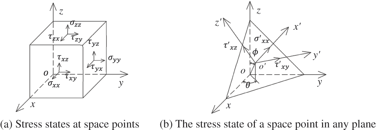
Figure 1: Three-dimensional plane stress transformation
If the expression of direction cosine is defined as Eq. (1), it is shown
The normal stress and strain after three-dimensional critical plane transformation can be expressed by Eqs. (2) and (3), respectively
The most disadvantage plane, also known as the critical plane, can be found through the transformed plane stress state.
Steps to determine the critical plane can be described as: first of all, divide a single load and unload analysis step into enough incremental steps, the number of incremental steps can describe the mechanical response changes under the action of a cyclic load in detail, and record the stress and strain information at the end of each incremental step, so as to obtain the historical changes of stress and strain under different loading cycles. Then, the node space is divided into the candidate critical planes according to a certain incremental angle (the incremental angle is selected as 5° in this paper), and the stress and strain information of each element is converted into a transformation formula, so as to obtain the stress and strain state of a point on any plane. Finally, through the states of these points, the damage parameters of each point in each plane are calculated, and the plane where the maximum value of the damage parameter is located is the critical plane.
A variety of fatigue life prediction models have been proposed based on different combinations of damage parameters on the critical plane [18]. However, due to the diversity of loading conditions, loading methods and structural forms, no model can be universally applied to all kinds of practical engineering. Smith et al. [19] believed that maximum stress controlled the impact of average stress on fatigue life under cyclic loading. Under a given fatigue life, the maximum stress
Therefore, in order to consider the impact of average stress on material fatigue life, Smith proposed SWT model on the basis of strain-life equation [3,19], namely, Eqs. (4) and (5), In this model, the product of the maximum strain amplitude and the maximum normal stress in the plane where the maximum strain amplitude is located is taken as the control parameter, denoted as SWT, as shown in Eq. (4). Suitable for tensile cracking as the main failure mode of materials.
where a complete cycle is defined as the process of the load increases from the minimum value to the maximum value and then decreases to the minimum value.
The multiaxial fatigue parameters of materials are the parameters measured in the complete alternating tension-compression fatigue test, including fatigue strength coefficient
The determination of multiaxial fatigue parameters needs to be based on a large number of fatigue tests. In the absence of relevant test data, Manson fitted the performance data of 29 materials and proposed the universal slope method [17]. Many scholars have proposed some methods to estimate parameter values based on uniaxial tensile test data of materials, such as Mitchell method, four-point correlation method, improved general slope method and median statistics method [20–24]. The fatigue performance parameters obtained by the general slope and median statistical method are shown in Table 1. In this paper, the required parameters are calculated by the median statistical method through trial calculation.
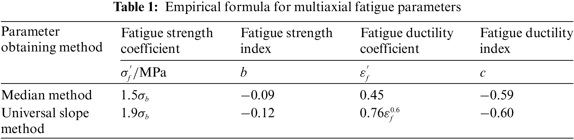
In the table,
2.3 Structure Solving Method Based on Cyclic Block
Since the fatigue life of the cable is very long in the real service environment, in order to improve the calculation efficiency, the solution strategy of “cyclic block” [25] is used in the simulation, a cyclic block is used to represent a certain number of loads, and it is considered that the characteristic values of material damage and elastic modulus remain unchanged in each cyclic block. As shown in Fig. 2, a cyclic block contains two analysis steps in the numerical simulation process, namely, a single loading analysis step and a single unloading analysis step. A cyclic block also corresponds to n times of loading in the actual project. In addition, when using the critical plane method in numerical simulation, single loading and unloading analysis steps should be divided into enough incremental steps to ensure the integrity of stress and strain data changes within a cyclic block [17]. The incremental step here is the calculation sub-step under the analysis step, and the load to be applied by an analysis step will be accumulated through these calculation sub-steps.
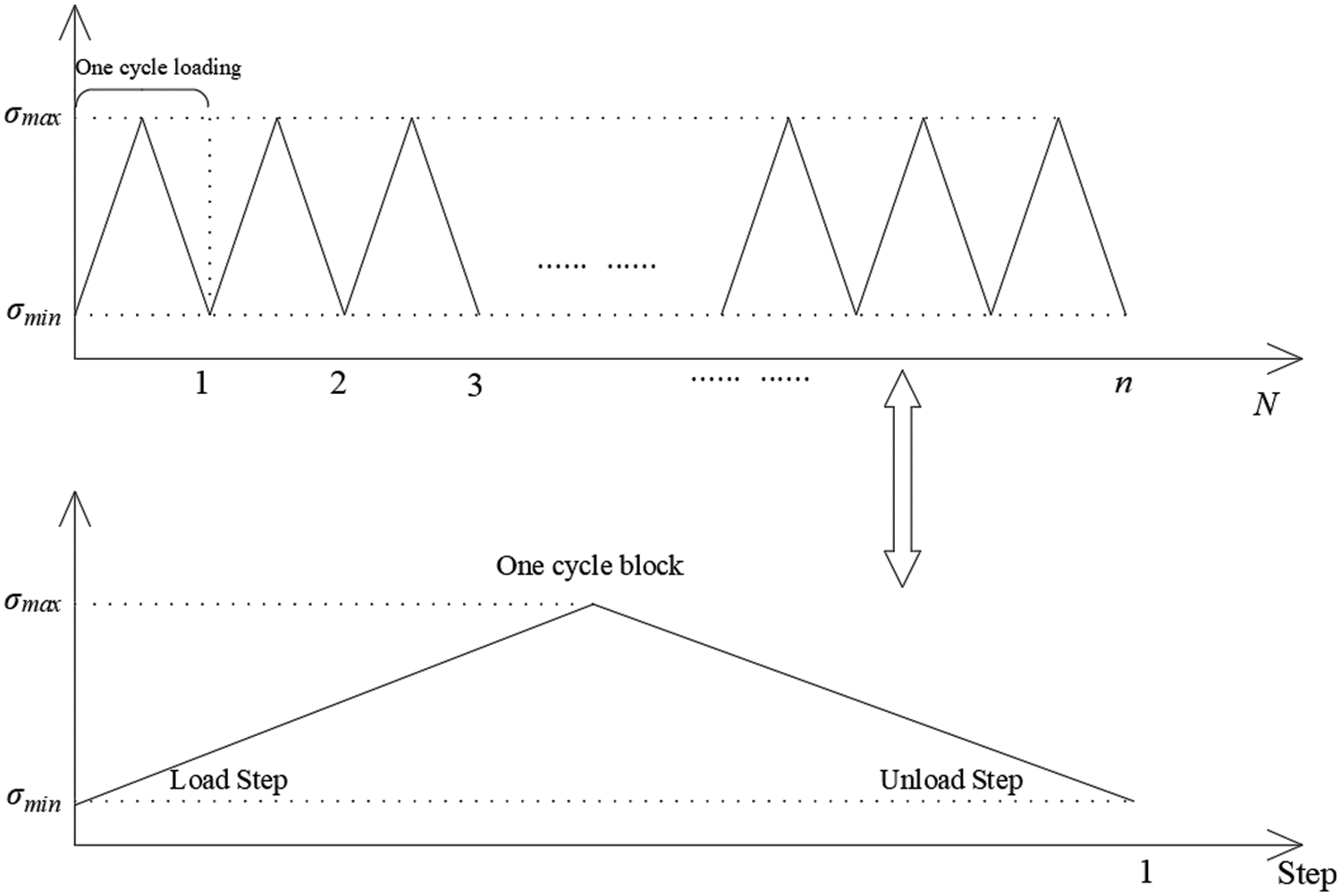
Figure 2: The relationship between cyclic blocks, analysis steps and number of loads
When the calculation proceeds to the next cyclic block, the eigenvalue of the material will be updated according to the state at the end of the previous cyclic block. Assume that the total number of loads in service are N; The actual number of loads contained in each cyclic block is denoting as
According to the theory of continuous damage mechanics, the damage accumulation of materials can be characterized by the reduction of elastic modulus of materials. In the evolution process of cable damage, when the first cyclic block starts, the initial damage is set as 0 and the initial elastic modulus is E. When the first cyclic block ends, the accumulated damage of the material is denoted as
At this point, the elastic modulus of the material can be expressed as Eq. (9):
According to the research on damage evolution theory in relevant literature [26], the damage threshold of the element is usually set as 0.9 or 1, that is, when the total damage value is greater than 0, it is considered that the element begins to be damaged; when the damage value reaches 0.9 or 1, it is considered that the element is completely invalid and will not participate in the subsequent finite element calculation. The damage threshold in this paper is 0.9.
2.4 Realization of Damage Model in Material Subroutine
SWT multiaxial fatigue model is used for analysis. In order to eliminate the influence of the critical plane changing with the cycle, when calculating the critical plane and damage value of each cyclic block, the position of the critical plane changing with the stress state is not considered, that is, the isotropic damage effect is assumed.
Fig. 3 shows the calculation method of damage increment in a cyclic block. Firstly, the loading and unloading analysis steps in a cyclic block need to be decomposed into enough incremental steps to ensure the integrity of stress and strain data changes in a cyclic block [17]. Through trial calculation, the analysis step length of a single loading/unloading process is specified as 20 steps. The stress and strain data of spatial points under each incremental step were recorded, and then the critical plane position and SWT values were calculated from these data. The life equation was solved and the damage increment within a single cyclic block was calculated. Finally, the required values were stored in the UMAT state variable.
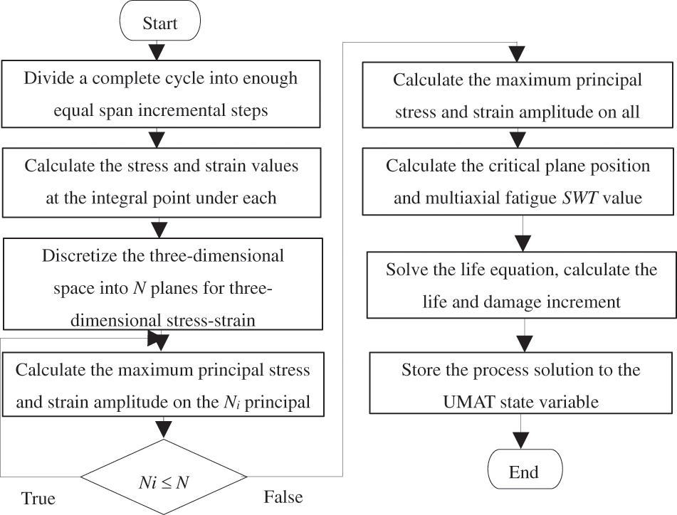
Figure 3: The calculation flow chart of damage increment of a complete cycle
Combined with the calculation method of damage increment within a single cyclic block, the technical route of damage evolution analysis is shown in Fig. 4. At the beginning of each analysis step, its properties are judged. For the first loading step, the material subroutine is called to solve the stress, strain and element damage value and other data, and stored in the corresponding state variables for the following calculation process. If it is the subsequent loading step, the solution process is the same as above, but the elastic modulus is no longer E, but the elastic modulus after damage accumulation which is considered as E × (1−D). If it is the unloading step, the state variables of adjacent loading steps are inherited, that is, it is assumed that the damage will not change in the unloading process. The above operations are repeated until the total damage of some elements reaches the damage limit, and then the failure of some elements is judged to have occurred in the material.
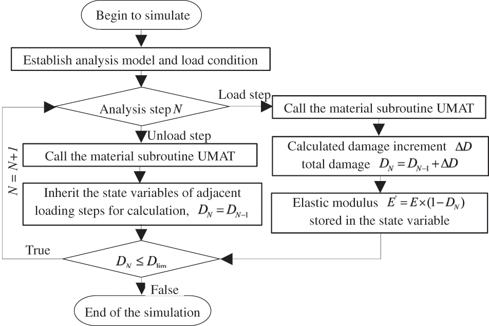
Figure 4: Implementation of damage evolution analysis
Considering that local plastic deformation will occur in the shallow surface near the contact surface, and the fretting damage on the surface has a great correlation with local plastic deformation, it is necessary to analyze the state of contact stress and local plastic deformation at the contact surface. Relevant results show that the selection of plastic constitutive relation has little influence on the amount of plastic deformation [17]. Therefore, in this paper, only isotropic elastic-plastic constitutive model without strengthening is preferred for material simulation.
The material custom user subroutine UMAT written according to the multiaxial fatigue damage model is shown in Fig. 5. The state variables set by the subroutine include elastic modulus, total damage, SWT, element life, elastic strain component, plastic strain component and equivalent plastic strain, as well as the calculated maximum strain value, minimum strain value and maximum normal stress in a single cyclic block.
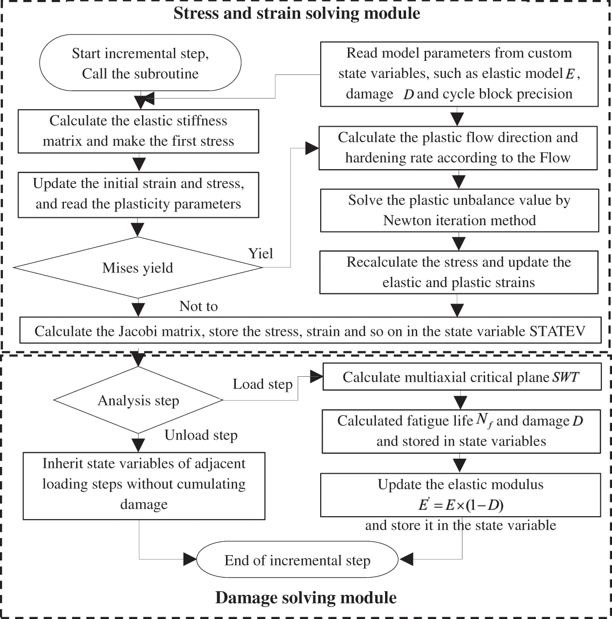
Figure 5: Realization method of material subroutine
The subprogram is divided into stress and in solving module and damage solving module. The former adopts the ideal elastic-plastic constitutive model, and the damage solving module is divided into the loading step and the unloading step. Thus, the custom state variable is updated at the end of each incremental step and returned to the main program to participate in the subsequent analysis step calculation. The damage increment is solved only at the last incremental step of each loading step, and it is assumed that the damage increment in the cyclic block needs to be calculated only at the end of the loading analysis step.
In fretting fatigue of the structure, interface slip, stress, strain and contact parameters are significantly greater than the rest of the region, the damage will be accumulated rapidly in the region, and most of the area of damage accumulation slower, which has less influence on the structure. Even in a considerable range, it will not lead to fatigue damage of the material, which means that the fatigue limit is not reached in this area. Therefore, a
2.5 Identification of Fretting Fatigue Failure of Materials
Corrosion fatigue life can be divided into corrosion fatigue crack nucleation life and corrosion fatigue crack growth life [27]. Corrosion fatigue crack nucleation includes three processes: the initiation of wear or pitting pits, the development of damage, and the conversion of wear or pitting to short cracks. While corrosion fatigue crack growth consists of four processes: the growth of short crack, the transformation of short crack to long crack, the growth of long crack and fracture [28]. Microcracks are easy to propagate and fracture under the action of fatigue loads, which is often studied by fracture mechanics [29]. In this study, when the material damage of cable wire contact surface and its subsurface reaches the critical value, it can be considered that the element in this area fails, and the initial crack is formed. The crack in this area can be simplified as type I crack under tensile load. The stress intensity factor in fracture mechanics theory can be used to characterize the stress field strength at crack tip of type I crack. When the stress intensity factor
where
2.6 Damage Theory of Fretting Fatigue and Corrosive Media
Corrosion fatigue damage refers to the damage caused by the mutual promotion of corrosion and fatigue behavior of materials under the joint action of cyclic load and corrosive medium. Compared with single fatigue or single corrosion, it will significantly accelerate the deterioration of mechanical properties on the surface and inside of materials. According to the theory of continuous damage mechanics, damage states in materials can be represented by macroscopic state variable D. D is also known as the damage parameter, which is a continuous internal thermodynamic variable used to describe the material degradation behavior during the increase of service time.
Under fretting fatigue alone and based on different combinations of damage parameters on the critical plane, various fatigue life prediction models have been proposed, such as SWT model introduced in Section 1.2. Fretting fatigue life can be expressed as Eq. (12):
The damage generated under single load is defined as Eq. (13):
where i is the i-th loading, and it is assumed that damage occurs only in the loading stage in this paper. Using linear damage accumulation Miner’s law, the total damage D was defined as Eq. (14):
In this paper, the damage limit D is set as 0.9, and it is believed that microcracks corresponding to the size of the element will occur when the current damage of the element reaches 0.9 [33].
In summary, this paper decomposed the causes of gradual failure of cable wire into three aspects, namely, the internal damage of unit caused by fretting fatigue, the change of contact surface morphology caused by wear, and the change of surface morphology caused by corrosion effect. The material damage caused by fretting fatigue and the change of surface morphology caused by corrosion wear promote each other with the increase of loading cycles, which leads to the rapidly deterioration and failure of cable.
3 Fretting Fatigue Damage Evolution Analysis of Cable Wire Considering Wear Morphology Evolution
3.1 Finite Element Model Establishment and Working Condition Setting
Fretting fatigue usually occurs between the outermost wires of adjacent cable strands during service. Therefore, in order to simplify the calculation, the two wires actually in contact were extracted from the steel strands model as the research object, and the finite element calculation model was established, as shown in Fig. 6a. A semi-symmetric structure is used for modeling, and the model includes a steel wire providing normal pressure and a steel wire bearing fatigue load. The diameter of the selected wire is 7 mm, and the length of the drawn wire is 100 mm.
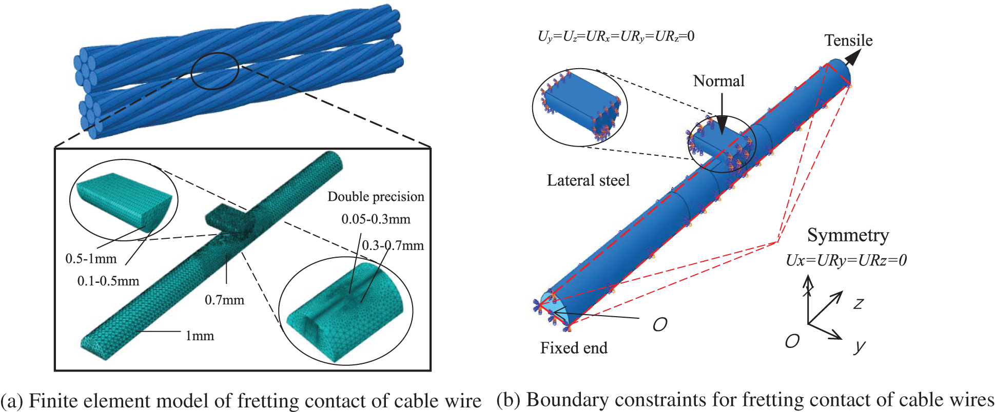
Figure 6: Finite element model and boundary condition of cable wire
The effective unity of computational efficiency and accuracy should be considered when meshing. In the non-critical area, four-node tetrahedral linear element (C3D4) was used, and the element size was set to about 1 mm. A six-node reduction integration element (C3D8R) is used in the key area, and the element size is transitioned from 0.05 to 1 mm. In order to achieve a good transition, the model is cut into regions. Although the C3D8R element is not the best element to calculate the contact problem, when the critical plane method is used to solve the life, the C3D8R element has only one internal integral point, so that the results of stress and strain can be directly used without special processing, which greatly reduces the post-processing workload. The contact area, marked by double precision of 0.05–0.3 mm as shown in Fig. 4a, the model adopts the double precision distribution method, so that the mesh is arranged from dense to sparse on the contact surface.
In order to simulate the actual stress state of cable wire, the loading mode and boundary conditions as shown in Fig. 6b are adopted. The origin O of the coordinate axis coincides with the centroid O' of the fixed-end section. The node constraint on the symmetry plane is Ux = URy = URz = 0. One end of the steel wire subjected to tensile load is set as the fixed end, the translation of the constraint node is in three directions, Ux = Uy = Uz = 0, and the other end is the loading end. The lateral wire limits all degrees of freedom except displacement in the x-axis direction, Uy = Uz = URx = URy = URz = 0. When applying constraints to the coupling points, the rotational constraints of the coupling points should be limited.
In solving the contact problem, it is necessary to define the contact pair and the normal and tangential action of the contact surface. The normal behavior of the model adopts hard contact, and the tangential behavior adopts penalty function method. Since there is only one set of contact pairs, the face-to-surface contact algorithm is selected to improve the computational efficiency. The lateral wire mesh is thicker, which is set as the main plane, and the tensile wire surface is set as the slave plane. For the finite element model of 90° steel wire contact, the friction coefficient is set as a constant value of 1.5 [34]. In practical engineering, there are many angles of steel wire intersection, only the simplified form of 90° arrangement is considered in this paper.
3.2 Verification of Material Subroutines
When there is normal contact force between the wires, the contact area will be in a multiaxial stress state, and the cable segment near the cable anchorage area is considered to be in a multiaxial stress state. In this section, a material subroutine based on fretting fatigue model was developed for the multiaxial fatigue condition. In order to explore the applicability of the subroutine to the damage evolution of cable steel wire, the life of steel wire under multiaxial fatigue condition is simulated and compared with the experimental results in the literature.
In literature [35], fretting fatigue tests with different fretting fatigue parameters were carried out on bridge cable wire, and it was found that the fretting fatigue failure was evolved from the microcrack on the trailing edge surface generated by the mixed slip zone. Fretting amplitude, friction coefficient and normal force are inversely proportional to fretting fatigue life. The elastic modulus of steel wire in the test is 202.5 GPa, yield strength, ultimate strength and elongation of crack were 1620, 1835 MPa and 5.78%, respectively, and the specimen length was 500 mm. The two ends are anchored by special fixtures, and the sinusoidal loading mode is used for displacement-based loading. Displacement loading is based on GB/T17101: steel wire with qualified fatigue performance should be able to resist 2 million fatigue cycles under the stress limit of
The multiaxial fatigue parameters were calculated by the median method, and the mechanical properties and parameters of materials were shown in Table 2. In addition, it is introduced above that the fracture toughness value of 7 mm high strength steel wire is about
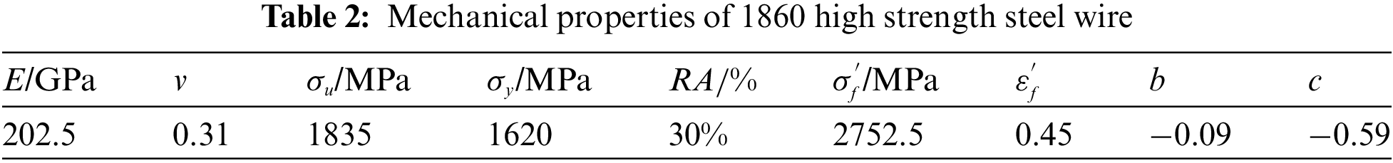
where E is the elastic modulus; v is Poisson’s ratio;
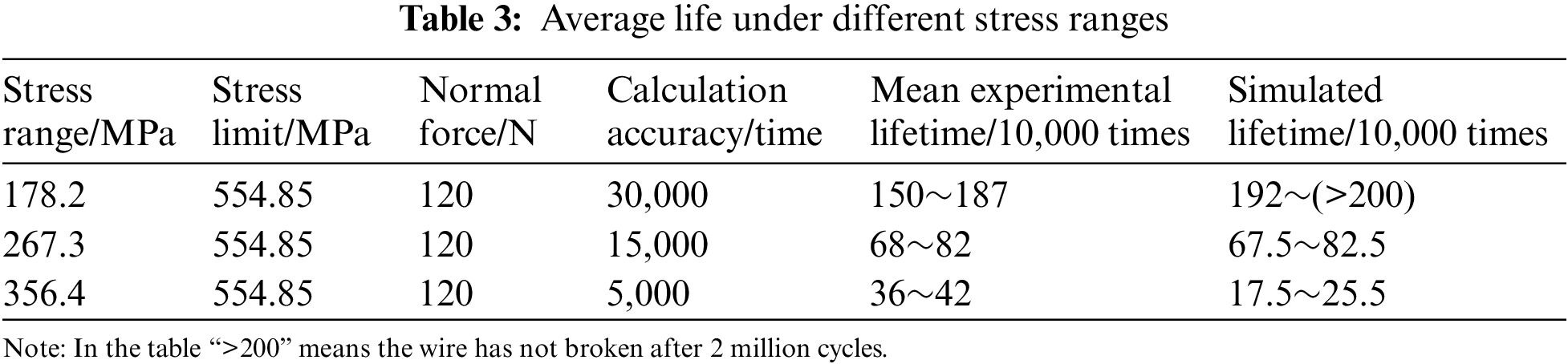
The test results and simulation results are shown in Table 3. Under fretting fatigue loads of different stress ranges, the numerical simulation life of the cable wire has the same trend as the test one. The error is only about 0.7% in the medium life area, the predicted value is larger in the high life area, and the predicted value is smaller in the low life area. Considering the influence of factors, such as the small amount of test data, the failure to completely reflect the properties of test materials and the multiaxial fatigue parameters, material appearance defects and process microdefects, the predicted life value is within the acceptable range, which can be used as the basis for subsequent research. It is considered that the applied fretting fatigue damage model of cable wires is reasonable and reliable, and can achieve the goal of predicting fretting fatigue life of cable wire.
3.3 Fretting Fatigue Evolution Simulation of Cable Wire Considering Wear Morphology Evolution
Fretting fatigue is often accompanied by severe wear behavior. The surface morphology evolution of materials changes with the increase of loading cycles, and the local stress and strain states change accordingly, resulting in local stress concentration and micro-plasticity, and aggravating the fatigue failure in key areas of materials. Experimental characterization of this phenomenon is often economically expensive and time-consuming. This paper attempts to investigate the effect of wear morphology evolution on the damage evolution of fretting fatigue of cable wire by numerical simulation.
Wear rate, also known as wear coefficient, is a physical quantity to measure the loss rate of materials in the wear process. The value is different in different materials or different fatigue loading stages of the same material. In order to simplify the calculation, this paper ignores the process of wear rate changes at the initial stage of loading and adopts constant wear rate throughout the whole numerical simulation process. In Wang’s [36] fretting fatigue test of high-strength steel wire, the wear rate of steel wire at 90° contact was measured, and the fixed value
3.3.1 Simulation Method of Cable Wire Surface Wear
ALE Adaptive Meshing Technology (Arbitrary Lagrangian-Eulerian Adaptive Meshing) can gradually improve the mesh quality without changing the original mesh topology. It is mainly used for simulation of large deformation, wear and erosion. In wear applications, a complete ALE process can be divided into several mesh repartitioning processes, and each mesh repartitioning process contains two steps. The first step is to generate a good mesh by using the algorithm and control strategy. The second step is to transfer the variable information in the old mesh to the new mesh by using Remapping Technology. Information about these variables can be the stress, strain, displacement or damage field concerned by the program.
UMESHMOTION is a subroutine module of Abaqus/Standard, used in conjunction with ALE Adaptive Meshing Technology to control the movement of nodes, often used for wear or ablation simulations. This subroutine is called at the end of any increment execution, and the amount of node movement is equal to the local amount of wear, so that the outer damage element will peel off under wear effect, thus simulating the surface mechanical damage caused by fretting fatigue. ALE technology then creates new meshes through a scanning process and remaps them from the old to the new, this process is known as “Advection”. Finally, according to the cyclic ending conditions that have been set, the above operations are repeated to achieve the adaptive update of material nodes.
ULOCAL (3), which represents the displacement or speed of the node along the z direction (depending on the definition in the model, it is defined as displacement in this paper), needs to be defined in UMESHMOTION. This value adopts the value of the stable wear stage in the fretting fatigue test of steel wire. For the convenience of combining finite element analysis, the formula of wear depth is introduced at the contact point (15) [37]:
where
Combined with wear subroutine and ALE Adaptive Meshing Technology, this paper simulates the wear and peeling off phenomenon of materials. Using the theory of “cyclic block”, it is assumed that parameters, such as contact pressure and slip distribution remain constant within each cycle. Fig. 7 is the flow chart of the implementation method of contact surface morphology updating. The stress and strain solving module and damage solving module have been introduced in detail in Section 1.4, the end of the two modules represents the end of the computation of the incremental step. The update of contact surface morphology needs to call the written UMESHMOTION_Wear subroutine at the end of each incremental step, and specify the displacement or speed of each node along a certain direction to this subroutine. In the process of numerical simulation of wear, the contact stress and slip of each node on the contact surface can be extracted, and the wear depth of each node along the contact normal direction can be calculated by using the wear model, which means the displacement of the node along a certain direction.
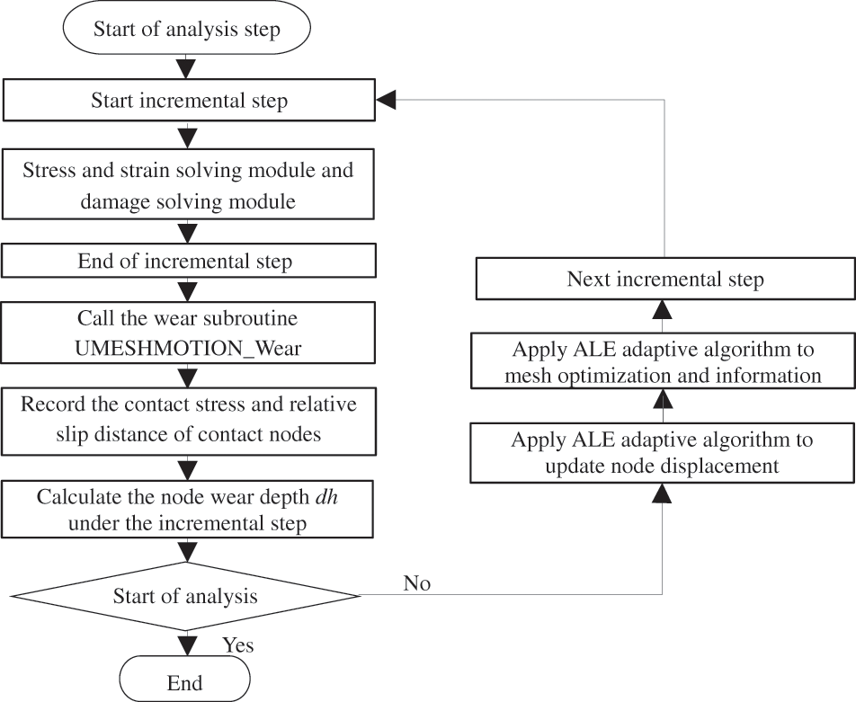
Figure 7: Flow chart of contact surface topography updating
3.3.2 Finite Element Model of Cable Wire Considering Wear Morphology Evolution
By comparing the wear tests of cable wire and finite element results in literature [16], it was found that the mesh size had no great influence on the contact pressure in the stable wear stage, but the optimal mesh size still needs to be studied to reduce computation time. Although the recommended mesh size is 3% to 4% of the final longitudinal wear width (6–8 microns), using a 24-micron mesh can reduce the computation time to 1/8 of the 6–8 microns. Therefore, considering the computation time and the reason that ALE technology cannot apply parallel computation, the minimum mesh size of 30 microns is used in the wear area.
In the finite element software ABAQUS, UMAT and UMESHMOTION_Wear subroutines can be used together to realize the mechanical behavior of material wear accompanied by damage accumulation. However, in the actual operation process, it is found that the wear algorithm will weaken the stress concentration phenomenon in the subsurface layer of the contact area, so as to weaken the fretting effect. Moreover, because the wear module can only use a single core for calculation, the calculation efficiency is low. Therefore, while using UMAT and UMESHMOTION_Wear coupling analysis, the wear behavior and damage behavior can also be simplified into two independent parts, and fretting fatigue damage calculation can be carried out on the cable wire with a certain stage of prewear.
The finite element model considering the evolution of wear morphology adopts the same model as that in Section 2.1, as shown in the Fig. 8.
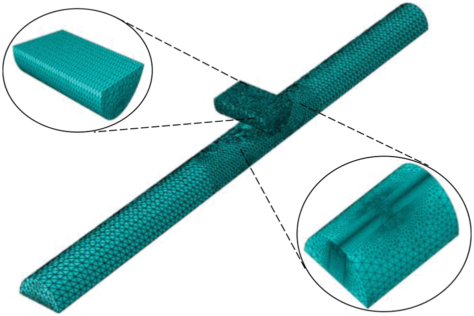
Figure 8: Finite element model considering wear morphology evolution
In this model, the stress lower limit of 554.85 MPa and the stress range of 267.3 MPa were adopted, and the normal loads were selected as 120, 180 and 240 N. The constraints and other settings are the same as in the model in Section 2.1. When using UMAT and UMESHMOTION_Wear coupling analysis, the calculation accuracy of normal load 120, 180 and 240 N is 30,000, 30,000 and 20,000 times, respectively.
3.3.3 Wear Morphology Evolution of Fretting Fatigue of Cable Wire
In order to study the change of fretting fatigue contact surface wear morphology of cable wire, the stress range 267.3 MPa, the lower limit of stress 554.85 MPa and the normal contact force 180 N were used as analysis conditions in this section, without considering the influence of fretting fatigue damage.
Fig. 9 shows the change of contact surface morphology with loading cycles. The strain diagram shown is the first incremental step of each loading analysis step, that is, at the beginning of loading. After 30,000 loads, the wear area presents an ellipse area, and gradually expands with the increase of the action cycle, which is the same as the wear area observed in the experiment. It proves that the wear subroutine developed can reasonably predict the wear behavior of the cable wire surface.
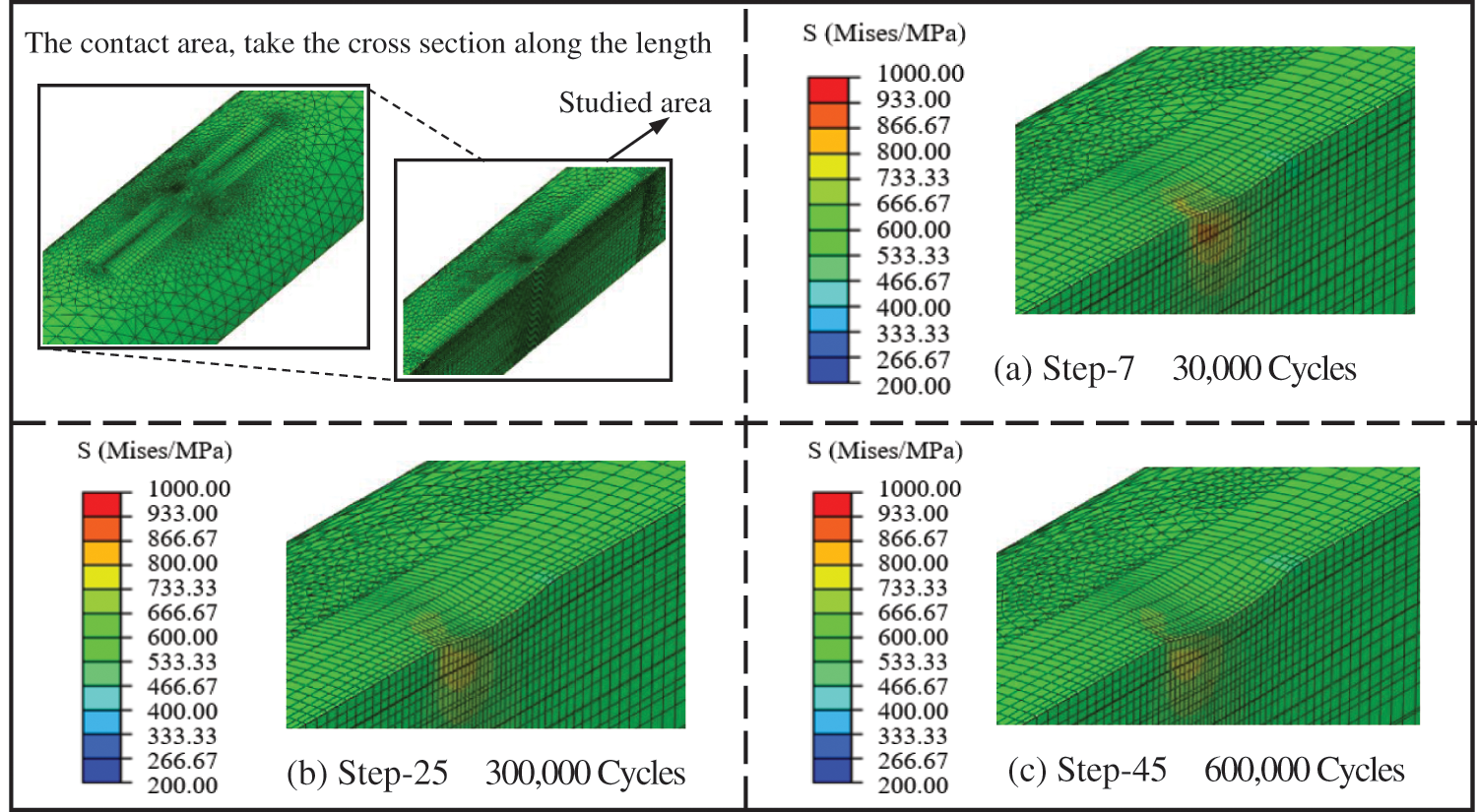
Figure 9: Wear appearance of contact surface
It should be noted that the maximum stress of Mises at 30,000 and 600,000 loads decreased with the increase of loading cycles, indicating that the stress concentration was weakened, which may be due to the influence of wear morphology evolution.
3.3.4 Fretting Fatigue Life Analysis of Cable Wire Considering Wear Morphology Evolution
Table 4 shows the fatigue life prediction of cable wire under fretting fatigue considering the evolution of wear morphology. It can be seen that, with the increase of the normal contact force, the fretting fatigue life generally presents a decreasing trend. The normal contact force increases from 120 N to 180 N and 240 N, and the fretting life is 690,000, 600,000 and 520,000 times, respectively. Compared with the normal contact force of 120 N, the fretting life decreases by 13% and 25%, respectively. This is because the increase of normal contact force has the effect of hindering the separation between wires, and leads to a significant increase of tangential stress, which then increases the stress and strain value of the material at the adhesive slip junction. Therefore, the increase of normal contact force can significantly reduce fretting fatigue life, and reasonable measures should be taken to reduce the friction between wires.
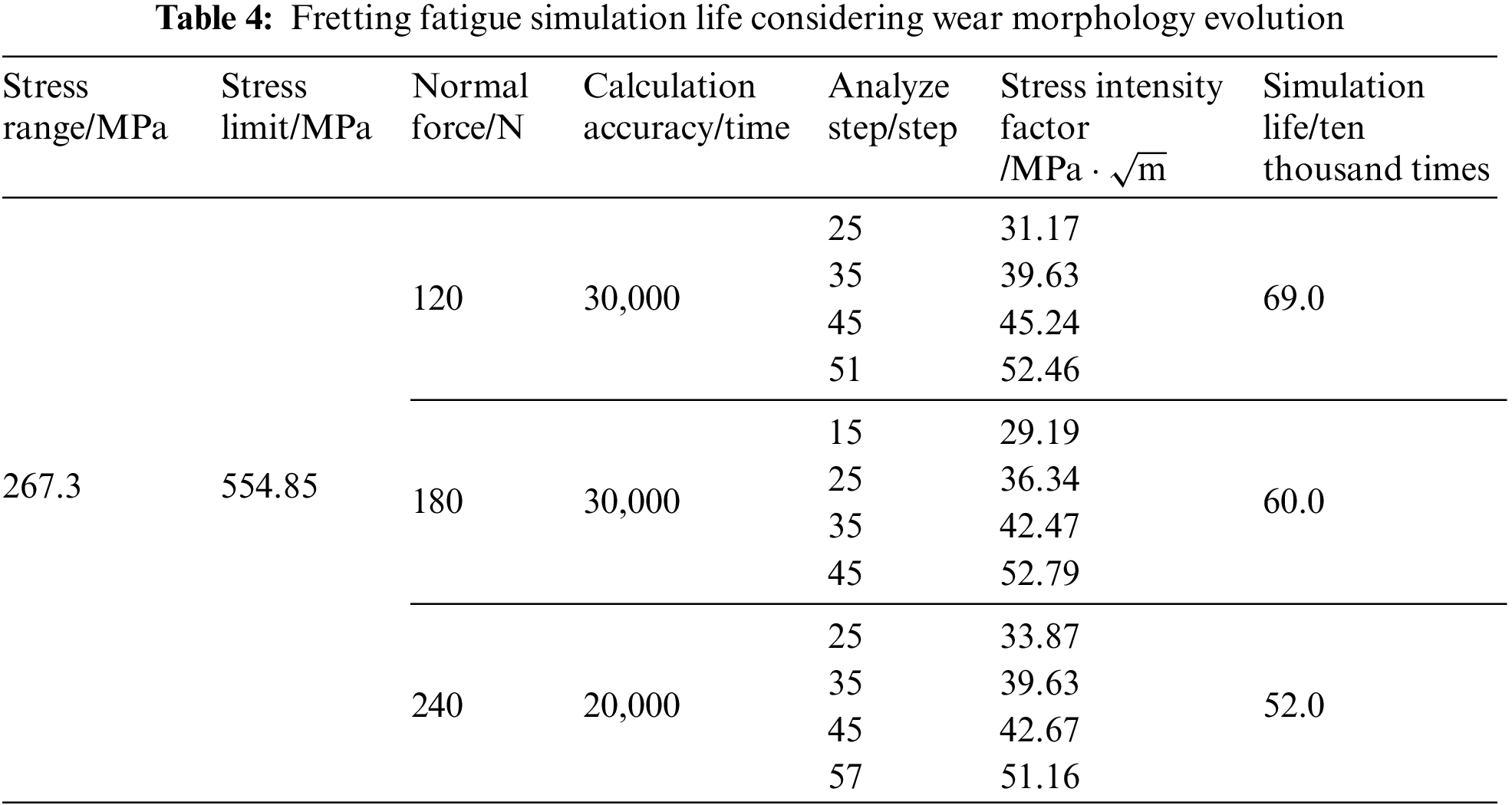
Fig. 10 shows the evolution of contact surface damage with the increase of loading cycles. At the initial stage of loading, with the increase of loading cycles, the damage on the contact surface of cable wire spreads along both the loop and contact slip directions, in this stage, the expansion rate along the loop direction is lower than that along the contact slip direction, and the damage limit area gradually occupies most of the contact area from the back edge of the contact area. At the late loading stage, the damage area spreads over the surface of the contact wear area, and the rate in the middle of the contact wear area expands to the wire loop direction, and the fretting fatigue life limit of the wire has been reached. This is related to the maximum section weakening effect and minimum effective section area at the midpoint of the wear zone when wear is considered.
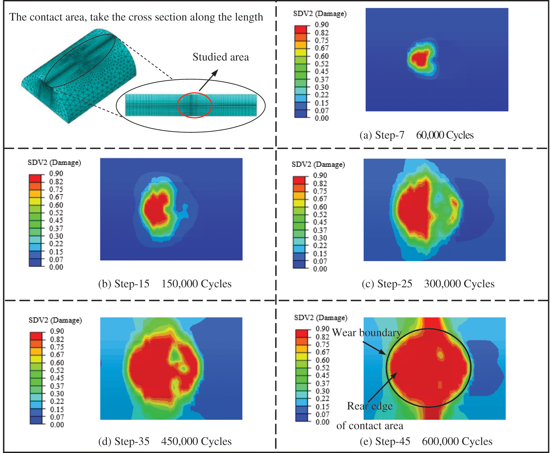
Figure 10: Evolution of contact surface damage with increasing loading cycles
Fig. 11 shows the damage evolution of fretting steel wire along the length direction z = 49.85 mm cross section. It can be found that the subsurface damage appears first at the initial stage of loading and reaches the damage limit preferentially. With the increase of loading cycles, it rapidly expands in a semi-elliptic shape along the radius direction. At the late loading stage, the materials at the contact part are gradually peeled off by wear behavior, leading to the rapid evolution of contact surface damage, rapid connection with the subsurface damage, forming macroscopic defects from surface to subsurface, and leading to brittle fracture of steel wire.
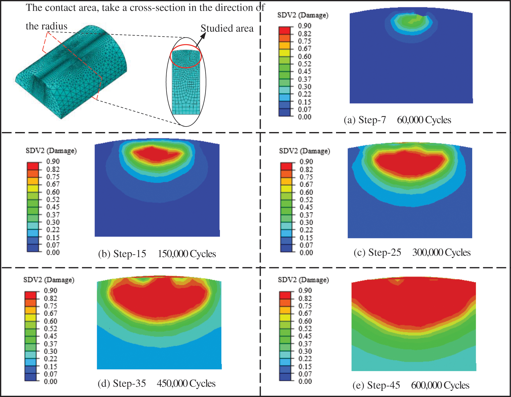
Figure 11: Damage evolution of cable cross section (z = 49.85 mm)
Fig. 12 shows the damage evolution of fretting wire along the length direction at y = 0 mm section. At the initial stage of loading, the damage limit was firstly reached at the back edge of the contact area and the subsurface of the contact area, and gradually connected with each other along the −45° direction with the increase of loading cycles. At the middle stage of loading, the damage continued to extend along the −45° direction to the inside of the steel wire, and also extended elliptically outwards on the cross section. In the middle and late stage of loading, the subsurface damage is rapidly connected with the contact surface damage, resulting in a weak area in the middle of the contact area, which also explains the two possible fracture locations in engineering practice.
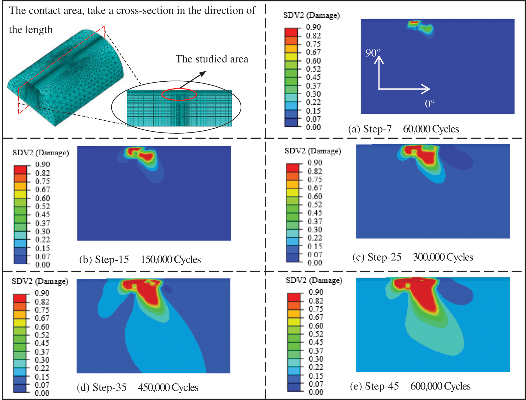
Figure 12: Damage evolution along the cable length section (y = 0 mm)
4 Damage Evolution Analysis of Cable Wire under Fretting Fatigue and Corrosion
When the galvanized layer on the surface of the cable wire is damaged, the passivation film on the surface of the wire will be further damaged, and corrosion will penetrate into the internal wire, forming a localized pitting pit. The mass loss rate of the material caused by local corrosion is small, but the stress concentration phenomenon will appear around the pit, and the stress concentration state will accelerate the growth process of the pit and greatly reduce the life of the cable.
Compared with conventional stress corrosion and corrosion fatigue, the service life of cable wires under fretting fatigue induced by wear is usually lower and the critical fatigue load is smaller. After the study of the replaced old cable, it is found that the surface morphology of the contact area is usually superimposed by wear morphology and corrosion morphology.
4.1 Erosion Pit Growth Model and Gutman Model
In the process of fretting fatigue, the wear behavior on the steel wire surface is easy to damage the surface passivation film. Then, chloride ions attach to the defects of the steel wire passivation film, react with cations to form soluble chloride, and form an active dissolution point at the damaged site of the passivation film. Therefore, the wear behavior creates conditions for accelerated corrosion. Literature [38] established a model of corrosion pit depth distribution of high strength steel changing with time, which was used to describe the rule of pitting pit depth
where
Fatigue is generally expressed by loading cycles, and each load corresponds to the time experienced in actual working conditions. Corrosion occurs in the whole life cycle of structure service process, which is discretized into: only calculate the corrosion depth and update the surface morphology at the end of each loading cycle. Assuming that after 10 days of loading 30,000 times in engineering practice, the corresponding stress-free pit depth increases by 0.01 mm. If the ratio of number of loads to time is defined as T, then the number of loads per day is 3,000. At this time, if the value of T increases to 6,000 times, it takes 5 days, and the corresponding pit depth is
where N is the total number of loads; T is the number of loads per unit time;
Gutman [39] found through research that stress, elastic deformation and plastic deformation can promote the anodic activity of metal, and thus proposed a model to describe the promotion effect of stress and strain state on electrochemical effect, hereinafter referred to as Gutman model. The expressions of materials in elastic stage and plastic stage are shown in Eqs. (20) and (21), respectively.
where I is the anode electric current under the stress field;
The above model shows that the electric current density varies with the magnitude of plastic strain, average stress, stress amplitude and other variables. Now, the ratio of anode current under load and no load is defined as “state acceleration factor
where
The material parameters used in this paper are shown in Table 5 [39].
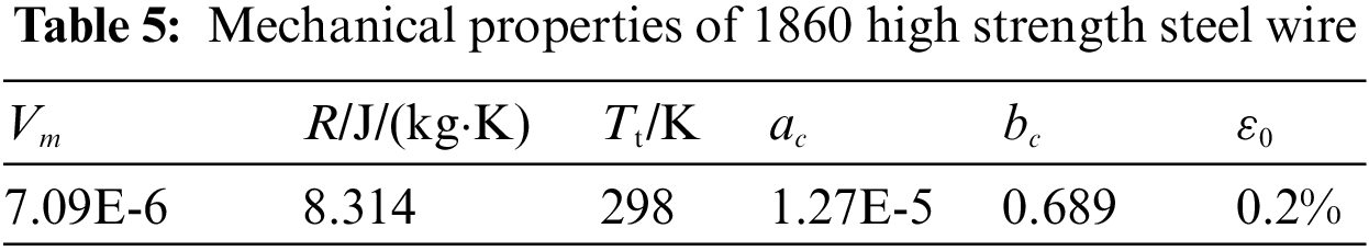
where
4.2 UMESHMOTION Subroutine Considering Both Wear and Corrosion Morphology Evolution
Fig. 13 is a subroutine implementation flow chart considering both wear and corrosion morphology evolution (this chapter relies on UMESHMOTION module of ABAQUS, and the subroutine developed is named UMESHMOTION_Wear_Corrosion). At the beginning, the main program first calls UMAT material subroutine to calculate the stress and strain. At the end of the solution, the main program calls the UMESHMOTION_Wear_Corrosion subroutine, which reads the contact stress, slip and elastic-plastic strain information from the calculation results to calculate the displacement of each node. The physical significance of the displacement is the wear depth and corrosion depth defined in the model. The wear depth and corrosion depth are simultaneously calculated in the subroutine and linearly superimposed at each node. Next, the main program receives the displacement of each node and updates the node position. Finally, the main program needs to use ALE adaptive mesh technology to optimize the mesh and morphology information, including stress, strain and cell damage data. When using ALE adaptive mesh, with the increase of cell deformation, the solver will gradually update the position of nodes and cells to avoid excessive cell deformation. At the same time, the solution variable will be transformed from the old cell mesh to the new cell mesh, and the position of the mesh and the position of the material point are no longer consistent.
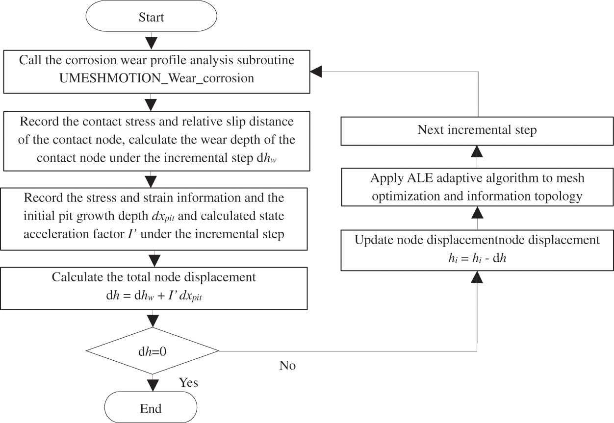
Figure 13: UMESHMOTION subroutine flow chart considering wear and corrosion effects
4.3 Numerical Simulation of Damage Evolution of Cable Wire Considering Wear and Corrosion Morphology Evolution
Wear and corrosion morphology evolution results in the formation of the contact surface defect, the defect cause local stress concentration, which in turn makes relevant material unit fast cumulative damage, then the increase of the damage lead to the change of stress and strain state, so as to accelerate the evolution of surface defects, the cycle of mutual promotion, accelerate the contact area of material loss, and weaken the section carrying capacity.
In order to study the morphologies and damage evolution of cable wire contact surfaces under different working conditions, constant wear rate
4.3.1 Contact Surfaces that Consider the Evolution of Wear and Corrosion Morphology
Fig. 14 shows the change of contact surface morphology with loading cycles considering the evolution of wear and corrosion morphology. The normal contact force is set as 120 N, and the number of loads per unit time is 50 times. With the increase of loading cycles, the depth and width of the wear area increase linearly. After 600,000 loads, the depth of the wear area is close to 0.08 mm.
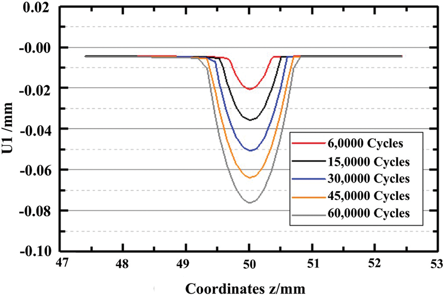
Figure 14: Diagram of contact surface changes considering wear and corrosion morphology evolution
Fig. 15 shows the comparison of contact surface morphology with different number of loads per unit time. The normal contact force is set as 120 N, the number of loads per unit time is 50, and the number of loads is 600,000. When
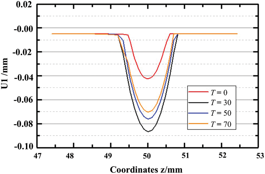
Figure 15: Comparison of contact surface morphology with wear and corrosion morphology evolution different number of loads per unit time (600,000 loads)
Fig. 16 shows the comparison of contact surface morphology considering different factors when loading 450,000 times. When only wear morphology evolution is considered, the material loss of contact surface is small. When both wear and corrosion morphologies are considered, the material loss along the depth direction increases significantly, but the depth loss changes little when the acceleration effect of force on corrosion is considered or not.
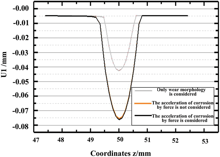
Figure 16: Comparison of contact surface morphology considering different working conditions (450,000 loads)
The possible main reasons are as follows: 1) For fretting fatigue, only a small fatigue load is required to cause fretting fatigue damage in the contact area, while the elastic acceleration factor caused by a load with a stress range of 267.3 MPa is only about 1.0000008 in the Gutman model. 2) The materials with micro-plastic contact surface peel off due to wear and corrosion behavior, so that the accelerated effect of plastic deformation on corrosion is greatly weakened. Therefore, it can be considered that the fretting fatigue effect is relatively small, and its acceleration effect on corrosion effect is limited. 3) The loading cycle is less, which fails to fully reflect the acceleration effect of force on corrosion.
4.3.2 Comparison of Fretting Fatigue Life Considering Wear and Corrosion Morphology Evolution
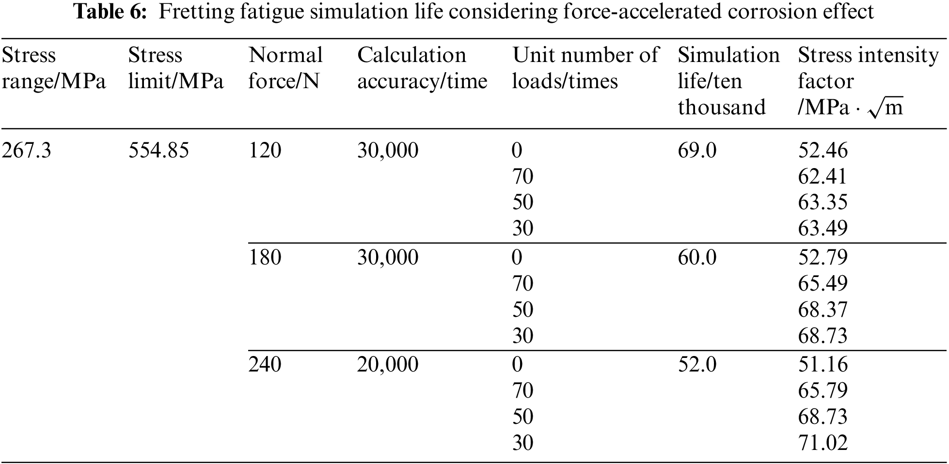
In the numerical simulation work considering wear and corrosion morphology changes, in order to give consideration to the calculation efficiency of single-core calculation, the value of calculation accuracy is large, and the change of life is not obvious. Therefore, the influence of force-accelerated corrosion on life was studied by comparing strength with strength at a certain life span. The results are shown in Table 6. When the normal contact force is 180 N, the stress range is 267.3 MPa, the stress limit is 554.85 MPa, the number of loads per unit time are 0, 70, 50 and 30, and the fretting fatigue life is 600,000 times, the stress intensity factors are 52.79, 65.79, 68.37 and 68.73
4.3.3 Damage Evolution Analysis Considering Wear and Corrosion Morphology Evolution
This section takes the contact cable wire in the stress range of 267.3 MPa, the lower limit of stress 554.85 MPa, the normal contact load of 120 N and the number of loads per unit time of 50 as an example. The corresponding test conditions are initial displacement of 1.37 mm, normal force of 120 N and displacement range of 0.66 mm. The damage evolution process of cable wire under fretting fatigue was studied.
Fig. 17 shows the evolution of cable wire contact surface damage with loading cycles. Compared with only considering the wear morphology evolution, the common denominator is: At the initial stage of loading, the element with damage limit appeared first at the back edge of the contact surface. Both of them would lead to the loss of the surface material of the contact area due to wear, weaken the effective bearing area of the section, intensify the stress concentration effect and produce elliptical damage zone at the back edge of the contact area. With the increase of loading cycles, the damage on the contact surfaces of both surfaces expands along the loop direction and the contact slip direction. At this stage, the expansion rate along the loop direction is lower than that along the contact slip direction, and the damage limit area gradually occupies most of the contact area from the back edge of the contact area. At the late loading stage, the damage area spreads over the surface of the contact wear area, and the rate in the middle of the contact wear area expands to the wire loop direction, and the fretting fatigue life limit of the wire has been reached.
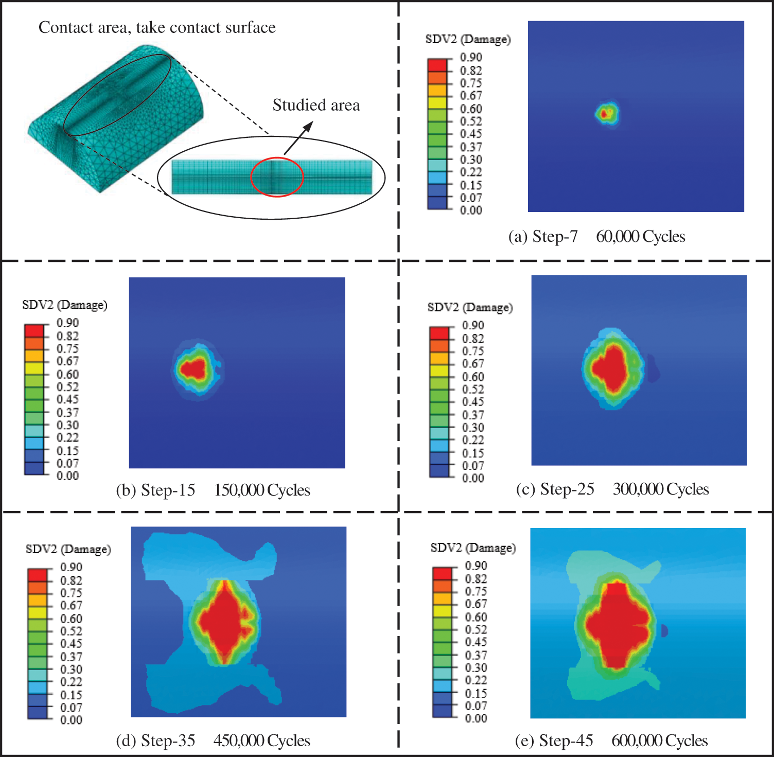
Figure 17: Damage evolution of contact surfaces
The differences are: When the evolution of wear and corrosion morphology was considered, the damage on the contact surface evolved to the bottom of the pit first. When loading for 300,000 times, the damage had covered the entire contact surface, which required loading for 450,000 times when only the evolution of wear morphology was considered. Similarly, when wear and corrosion morphology changes are considered, a penetrating damage zone has been formed in the observation area when the wear and corrosion morphology changes are considered for 450,000 times, while the number of loads are 600,000 when the wear morphology evolution is considered only. Obviously, considering wear and corrosion morphology changes, the fatigue life of cable wires can be significantly reduced. When only the evolution of wear morphology is considered, it has been shown that the damage region in the subsurface layer of the contact area will be connected with the damage in the subsurface layer, forming a macroscopic crack located in the middle of the wear area, and finally leading to the brittle fracture process of steel wire. When the evolution of corrosion and wear morphology is considered simultaneously, the peeling off process of materials on the contact surface will be accelerated, so that the subsurface damage can be directly transformed into surface damage, which shortens the process of interpenetration, and also significantly accelerates the fretting fatigue failure of cable wires.
Fig. 18 shows the damage evolution of fretting wire along the length direction at the cross section z = 49.85 mm. It is the same as that when only wear morphology evolution is considered, the subsurface damage reaches the damage limit preferentially at the initial stage of loading, and rapidly develops in a semi-elliptic shape along the radius direction with the increase of loading cycles. The difference is that when wear and corrosion morphologies are considered, the subsurface damage evolves into surface damage after only 300,000 loads, while when wear morphologies are considered only, the contact surface damage and subsurface damage tend to be interconnected after 450,000 loads.
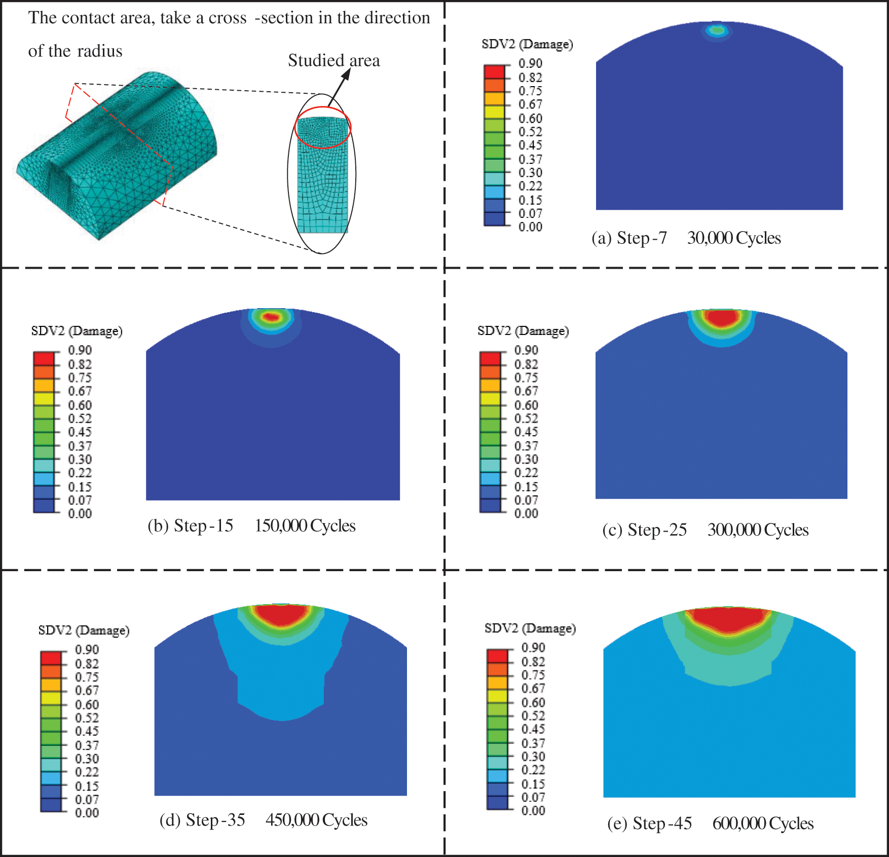
Figure 18: Damage evolution of cross section along cable length (z = 49.85 mm)
Fig. 19 shows the damage evolution of fretting steel wire along the length direction, y = 0 mm section. The change of contact surface morphology can be clearly observed in this direction. It is the same as that when only the wear morphology evolution is considered: At the initial stage of loading, the damage limit was first reached at the back edge of the contact area, and then extended to the inside of the steel wire along the direction of −45° with the increase of loading cycles. The differences are: The damage evolution rate is significantly accelerated when the wear and corrosion morphologies are considered. The process of surface damage and subsurface damage is replaced by wear and corrosion process, and the damage rapidly evolves from the back edge of the contact area to the bottom of the wear corrosion pit, and spreads along −45°, forming a penetrating crack, leading to brittle fracture of cable wire.
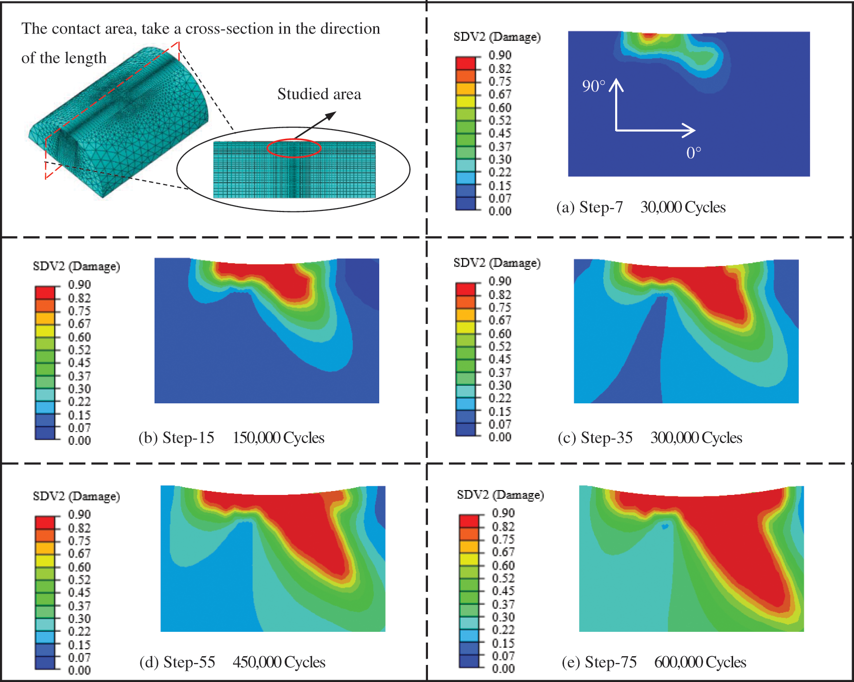
Figure 19: Damage evolution along cable length considering corrosion and wear effects (y = 0 mm profile)
In this paper, fretting fatigue damage evolution constitutive models are established, which consider the evolution of wear morphology and the evolution of wear and corrosion morphology. The corresponding subroutines UMESHMOTION_Wear and UMESHMOTION_Wear_Corrosion were written to visualize the damage evolution process of cable wire respectively, and the fretting fatigue life prediction was realized. The following conclusions were obtained:
(1) Based on the material custom user subroutine developed in this paper, the numerical simulation and visualization of fretting fatigue damage evolution of three-dimensional structures can be realized. The SWT model applied in this paper has good applicability to the fretting fatigue simulation of the cable wire.
(2) When the normal contact is 180 and 240 N, the fretting fatigue life of the wire rope is 13% and 25% lower than that of 120 N, respectively. Therefore, reasonable measures need to be taken to reduce the friction between the wires.
(3) When both wear morphology and corrosion effects are considered, the depth of the wear area exceeds 0.08 mm after 600,000 loadings, which is much greater than 0.04 mm when corrosion effects are not considered. The corrosion effect will significantly increase the total rate of material loss on the contact surface.
(4) Compared with the case where only the wear morphology evolution is considered. The depth of material loss increases significantly when considering the wear and corrosion morphology changes. However, the acceleration effect of force on corrosion has little effect on material loss.
(5) When only the wear morphology evolution is considered, the cable wire undergoes 450,000 loadings when the damage covers the entire contact surface, and 600,000 loadings when a through damage zone is formed, while only 300,000 and 450,000 loadings are required when considering both the wear and corrosion morphology evolution, respectively. The effect of wear and corrosion morphological evolution accelerates the damage fracture process of the cable wire.
(6) Compared with only considering the evolution of wear morphology, the damage evolution of the contact surface is preferred to the bottom of the wear pit and evolves at a faster rate along the −45° direction when considering the change of wear and corrosion morphology. The evolution of corrosion pits and wear morphologies leads to stress concentration in the contact zone, which in turn accelerates the evolution of corrosion and wear morphologies.
Funding Statement: The works described in this paper are substantially supported by the grant from National Key Research and Development Program of China (Grant No. 2021YFF0602005) and National Natural Science Foundation of China (No. 51678135), which are gratefully acknowledged.
Conflicts of Interest: The authors declare that they have no conflicts of interest to report regarding the present study.
References
1. Zhao, B. F., Xie, L. Y., Xu, G. L., Li, H. Y., Zhang, S. J. et al. (2017). Multiaxial fatigue life prediction method. Failure Analysis and Prevention, 12(5), 323–330. [Google Scholar]
2. Zhou, W. (2007). Fretting fatigue crack initiation characteristics and life prediction (Master Thesis). Zhejiang University of Technology, China. [Google Scholar]
3. Sum, W. S., Williams, E. J., Leen, S. B. (2005). Finite element, critical-plane, fatigue life prediction of simple and complex contact configurations. International Journal of Fatigue, 27(4), 403–416. DOI 10.1016/j.ijfatigue.2004.08.001. [Google Scholar] [CrossRef]
4. Hu, J. Y. (2018). Study on fretting slip behavior of parallel steel wires of stay cables (Master Thesis). Changsha University of Science and Technology, China. [Google Scholar]
5. Rokhlin, S. I., Kim, J. Y., Nagy, H., Zoofan, B. (1999). Effect of pitting corrosion on fatigue crack initiation and fatigue life. Engineering Fracture Mechanics, 62(4–5), 425–444. DOI 10.1016/S0013-7944(98)00101-5. [Google Scholar] [CrossRef]
6. Lan, C. M., Xu, Y., Liu, C. P., Li, H., Spencer, B. F. et al. (2018). Fatigue life prediction for parallel-wire stay cables considering corrosion effects. International Journal of Fatigue, 114(9), 81–91. DOI 10.1016/j.ijfatigue.2018.05.020. [Google Scholar] [CrossRef]
7. Li, R., Miao, C. Q., Feng, Z. X., Wei, T. H. (2021). Experimental study on the fatigue behavior of corroded steel wire. Journal of Constructional Steel Research, 176, 106375. DOI 10.1016/j.jcsr.2020.106375. [Google Scholar] [CrossRef]
8. Li, X. M., Zhou, J. M., Liu, Q., Kong, L. F., Zhou, J. T. (2007). Effect of tension on corrosion behavior of galvanized steel strand in cable-stayed bridge cables. Electrochemical, (3), 297–301. [Google Scholar]
9. Wang, Y., Yan, Z., Wang, Z. (2021). Fatigue crack propagation analysis of orthotropic steel bridge with crack tip elastoplastic consideration. Computer Modeling in Engineering & Sciences, 127(2), 549–574. DOI 10.32604/cmes.2021.014727. [Google Scholar] [CrossRef]
10. Wang, Y., Shi, H. R., Ren, S. B. (2021). Cellular automata simulations of random pitting process on steel reinforcement surface. Computer Modeling in Engineering & Sciences, 128(3), 967–983. DOI 10.32604/cmes.2021.015792. [Google Scholar] [CrossRef]
11. Yu, Y., Sun, Z. Z., Wang, H. K., Gao, J., Chen, Z. W. (2022). Time variant characteristic of steel cable considering stress-corrosion deterioration. Construction and Building Materials, 328, 127038. DOI 10.1016/j.conbuildmat.2022.127038. [Google Scholar] [CrossRef]
12. Wang, H. K., Yu, Y., Xu, W. P., Li, Z. M., Yu, S. Z. (2021). Time-variant burst strength of pipe with corrosion defects considering mechano-electrochemical interaction. Thin-Walled Structures, 169, 108479. DOI 10.1016/j.tws.2021.108479. [Google Scholar] [CrossRef]
13. Wang, H. K., Gao, J., Liu, T., Yu, Y., Xu, W. P. et al. (2022). Axial buckling behavior of H-piles considering mechanical-electrochemical interaction induced damage. Marine Structures, 83, 103157. DOI 10.1016/j.marstruc.2022.103157. [Google Scholar] [CrossRef]
14. Xu, L. Y., Cheng, F. (2017). A finite element based model for prediction of corrosion defect growth on pipelines. International Journal of Pressure Vessels and Piping, 153, 70–79. DOI 10.1016/j.ijpvp.2017.05.002. [Google Scholar] [CrossRef]
15. Ma, L. (2000). Study on fatigue performance of 1860 low-relaxation prestressed steel strand made in China. Railway Standard Design, 20(5), 3. [Google Scholar]
16. Cruzado, A., Leen, S. B., Urchegui, M. A., Gomez, X. (2013). Finite element simulation of fretting wear and fatigue in thin steel wires. International Journal of Fatigue, 55, 7–21. DOI 10.1016/j.ijfatigue.2013.04.025. [Google Scholar] [CrossRef]
17. Guo, T. T. (2015). Simulation research on multi-axis fatigue life of key parts of diesel engine block (Master Thesis). North University of China, China. [Google Scholar]
18. Yang, Q., Cheng, J. H., Guan, H. J., Tan, W. J. (2020). Research progress of fretting fatigue damage theory. Internal Combustion Engine and Parts, (3), 220–221. [Google Scholar]
19. Smith, K. N., Topper, T., Watson, P. (1970). A stress–strain function for the fatigue of metals (stress-strain function for metal fatigue including mean stress effect). Journal of Materials, 5, 767–778. [Google Scholar]
20. Zhang, Z. S. (2014). Fatigue life prediction and dynamic reliability analysis of aero-engine turbine disc (Master Thesis). University of Electronic Science and Technology of China, China. [Google Scholar]
21. Meggiolaro, M. A., Castro, J. T. P. (2004). Statistical evaluation of strain-life fatigue crack initiation predictions. International Journal of Fatigue, 26(5), 463–476. DOI 10.1016/j.ijfatigue.2003.10.003. [Google Scholar] [CrossRef]
22. He, J. R. (2004). Metal fatigue at high temperature. Beijing, China: Science Press. [Google Scholar]
23. Distefano, S., Puliafito, A. (2006). System modeling with dynamic reliability block diagrams. European Safety and Reliability Conference, pp. 569–575. Estoril, Portugal. [Google Scholar]
24. Hollander, M., Pena, E. A. (1995). Dynamic reliability models with conditional proportional hazards. Lifetime Data Analysis, 1, 377–401. DOI 10.1007/BF00985451. [Google Scholar] [CrossRef]
25. Wang, Y. (2019). Simulation of damage evolution and study of multi-fatigue source fracture of steel wire in bridge cables under the action of pre-corrosion and fatigue. Computer Modeling in Engineering & Sciences, 120(2), 375–419. DOI 10.32604/cmes.2019.06905. [Google Scholar] [CrossRef]
26. Sun, X. X. (2016). Numerical simulation of fatigue crack growth of concrete under cyclic loading (Master Thesis). Southeast University, China. [Google Scholar]
27. Huang, X. G. (2013). Corrosion fatigue pitting development and crack propagation mechanism (Master Thesis). Shanghai Jiao Tong University, China. [Google Scholar]
28. Zheng, Y. Q. (2019). Study on the damage and deterioration process of cable steel wire under the coupling effect of corrosion and fatigue (Master Thesis). Southeast University, China. [Google Scholar]
29. Wei, X. L., Makhloof, D. A., Ren, X. D. (2023). Analytical models of concrete fatigue: A state-of-the-art review. Computer Modeling in Engineering & Sciences, 134(1), 9–34. DOI 10.32604/cmes.2022.020160. [Google Scholar] [CrossRef]
30. Fu, X. J. (1995). Structural fatigue and fracture. Xi’an, China: Northwestern Polytechnical University Press. [Google Scholar]
31. Mahmoud, K. M. (2007). Fracture strength for a high strength steel bridge cable wire with a surface crack. Theoretical and Applied Fracture Mechanics, 48(2), 152–160. DOI 10.1016/j.tafmec.2007.05.006. [Google Scholar] [CrossRef]
32. Duquesnay, D. L., Underhill, P. R., Britt, H. J. (2003). Fatigue crack growth from corrosion damage in 7075-t6511 aluminium alloy under aircraft loading. International Journal of Fatigue, 25(5), 371–377. DOI 10.1016/S0142-1123(02)00168-8. [Google Scholar] [CrossRef]
33. Madge, J. J., Leen, S. B., Shipway, P. H. (2008). A combined wear and crack nucleation–propagation methodology for fretting fatigue prediction. International Journal of Fatigue, 30(9), 1509–1528. DOI 10.1016/j.ijfatigue.2008.01.002. [Google Scholar] [CrossRef]
34. Jia, R. Z., Wang, C. J. (2020). Analysis of fretting fatigue characteristics of steel strand cables based on SWT method. Mechanics Quarterly, 41(4), 657–665. [Google Scholar]
35. Guo, T., Liu, Z. X., Correia, J., de Jesus, A. M. P. (2020). Experimental study on fretting-fatigue of bridge cable wires. International Journal of Fatigue, 131(2), 105321. DOI 10.1016/j.ijfatigue.2019.105321. [Google Scholar] [CrossRef]
36. Wang, D. G. (2012). Fretting damage behavior and fretting fatigue life prediction of steel wire (Master Thesis). China University of Mining and Technology, China. [Google Scholar]
37. Madge, J. J., Leen, S. B., Mccoll, I. R., Shipway, P. H. (2007). Contact-evolution based prediction of fretting fatigue life: Effect of slip amplitude. Wear, 262(9–10), 1159–1170. DOI 10.1016/j.wear.2006.11.004. [Google Scholar] [CrossRef]
38. Turnbull, A., Mccartney, L. N., Zhou, S. (2006). A model to predict the evolution of pitting corrosion and the pit-to-crack transition incorporating statistically distributed input parameters. Environment-induced cracking of materials. Corrosion Science, 45(8), 2084–2105. DOI 10.1016/j.corsci.2005.08.010. [Google Scholar] [CrossRef]
39. Gutman, E. M. (1998). Mechanochemistry of materials. London, Cambridge: Int Science Publishing. [Google Scholar]
Cite This Article
 Copyright © 2023 The Author(s). Published by Tech Science Press.
This work is licensed under a Creative Commons Attribution 4.0 International License , which permits unrestricted use, distribution, and reproduction in any medium, provided the original work is properly cited.
 Downloads
 Citation Tools