
 Submit a Paper
 Propose a Special lssue
 Open Access
ARTICLE

A Numerical Investigation Based on Exponential Collocation Method for Nonlinear SITR Model of COVID-19
1 Department of Applied Mathematics, Imam Khomeini International University, Qazvin, 34149, Iran
2 Department of Mathematics, Faculty of Science, Akdeniz University, Antalya, 07058, Turkey
* Corresponding Authors: Saeid Abbasbandy. Email: ,
Computer Modeling in Engineering & Sciences 2023, 136(2), 1687-1706. https://doi.org/10.32604/cmes.2023.025647
Received 23 July 2022; Accepted 28 September 2022; Issue published 06 February 2023
 View Full Text
 Download PDF
Abstract
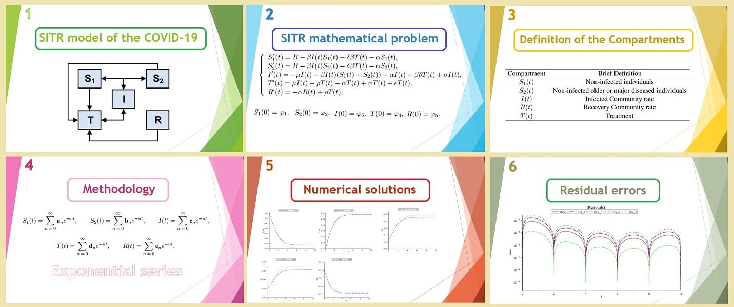
In this work, the exponential approximation is used for the numerical simulation of a nonlinear SITR model as a system of differential equations that shows the dynamics of the new coronavirus (COVID-19). The SITR mathematical model is divided into four classes using fractal parameters for COVID-19 dynamics, namely, susceptible (S), infected (I), treatment (T), and recovered (R). The main idea of the presented method is based on the matrix representations of the exponential functions and their derivatives using collocation points. To indicate the usefulness of this method, we employ it in some cases. For error analysis of the method, the residual of the solutions is reviewed. The reported examples show that the method is reasonably efficient and accurate.Graphic Abstract
Keywords
The world has recently contracted the dangerous and deadly disease coronavirus 2019 (COVID-19), which is an almost uncontrollable respiratory infection. The new coronavirus was reported in Wuhan, China in December 2019. The World Health Organization (WHO) announced the global pandemic of the infection in March 2020. Its disease pattern is called COVID-19 [1]. This disease that is highly contagious and through droplets can be transmitted from person to person. Many people are infected with COVID-19 and the number of victims of this virus is increasing every day. The COVID-19 spread ratio is very problematic and a concern for the whole world. The main cause of the spread of this virus is the contact of an infected person with healthy people, because studies have shown that this infection is usually caused by the transmission of blood cells through coughing or sneezing. These blood cells can stay in the air for a long time and cause infections for others. However, it is very challenging for scientists to study the preventive measures that can be taken to control the spread of the virus and to develop a vaccine to fight the virus. How to control the disease is one of the most important challenges if it is transmitted to animals or birds. Researchers are developing a variety of tactics to study the growing behavior of the coronavirus, and are studying ways to end COVID-19. Much research has been done to determine the conditions under which this deadly virus can be controlled. Scientists have found that COVID-19 is one of the most important outbreaks that attacks the respiratory system. One of the main reasons for the prevalence of COVID-19 is due to the transmission of germs through the respiratory cells in humans, and this virus is considered as a vector of transmission. The World Health Organization (WHO) has warned that the outbreak of the coronavirus could spread more rapidly if control measures were not implemented in a timely manner. WHO has advised people to stay away from infectious people or animals, including fever or any respiratory problems, and to recommend the use of surgical masks and the continued use of hand sanitizers in public places to protect oneself from infection. Social distance or less crowded places can reduce the risk of spreading the corona virus because it is more likely to spread in crowded places. The use of epidemiological computational simulation models plays a main role in estimating the transmission parameters and guessing the effective behavior of the infection. These models have been shown to be useful in depicting the growth rate or rate of decay of viruses over time. And they are very useful in providing control measures that can be adapted to reduce the spread of the disease. Many results and applications of COVID-19 simulation models are accepted and published [2–9]. Providing a mathematical model is another matter, while predicting the consequences of the disease is also very disappointing. One method of analyzing the behavior of diseases is divisional modeling, which can be used for mathematical models related to affective diseases. An appropriate vaccine must be discovered to prevent further damage of the virus. Otherwise, the world must be prepared to face many new challenges such as human casualties, food shortages, poverty, unemployment and so on.
One way to study the effective growth of this deadly outbreak is to use computer simulation block models. In different researches, different numerical and analytical approaches have been considered to perform the outputs of SITR models [10–13].
Differential equations have a remarkable role in several scientific and engineering phenomena that have always been considered at physical and technical applications and they are appeared in various areas as mathematics, physics and engineering sciences [14–17].
In recent years, Yüzbaşi et al. have applied the collocation method based on exponential approximation to solve some problems like pantograph equation, the linear neutral delay differential, Fredholm integro-differential difference equations and so on [18–21].
The aim of the present work is to find a numerical solution for a nonlinear SITR model using the new dynamic parameters of COVID-19, along with numerical analysis to better understand the expansion using numerical approaches through exponential basis.
The organization of this article is structured as follows: In Section 2, mathematical modelling of the SITR system is presented. In Section 3, we express briefly required mathematical elementary and matrix relations for exponential functions of the method. In Section 4, we present the numerical implementation of the matrix operation of the method. Section 5 involves the error analysis. For this purpose, assuming the residual of solution of Eq. (1). Section 6 contains numerical examples, where approximate solutions corresponding to various N values are obtained using the proposed method. Numerical experiments are examined to illustrate the efficiency and accuracy of the method, and results are reported. Finally, the last section consists of a brief conclusion.
Mathematical modelling of the dynamical system is an interesting field of study that has attracted most researchers’ attention. Dynamical systems have a wide range of applications, including population growth models, biomedical research, biological systems, and engineering.
In this approach, for the SITR model is designed for the new COVID-19 dynamics, the population is allocated to various compartments with particular labels, susceptible (S), infected (I), treatment (T), and recovered (R). The S is divided into
The SITR model of the novel COVID-19 dynamics is given by the following nonlinear 1st order differential equations and the description of each compartment is given in Table 1.
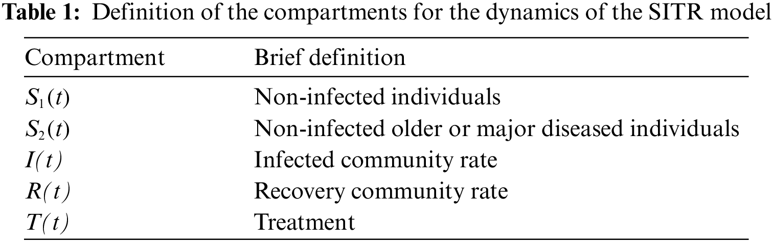
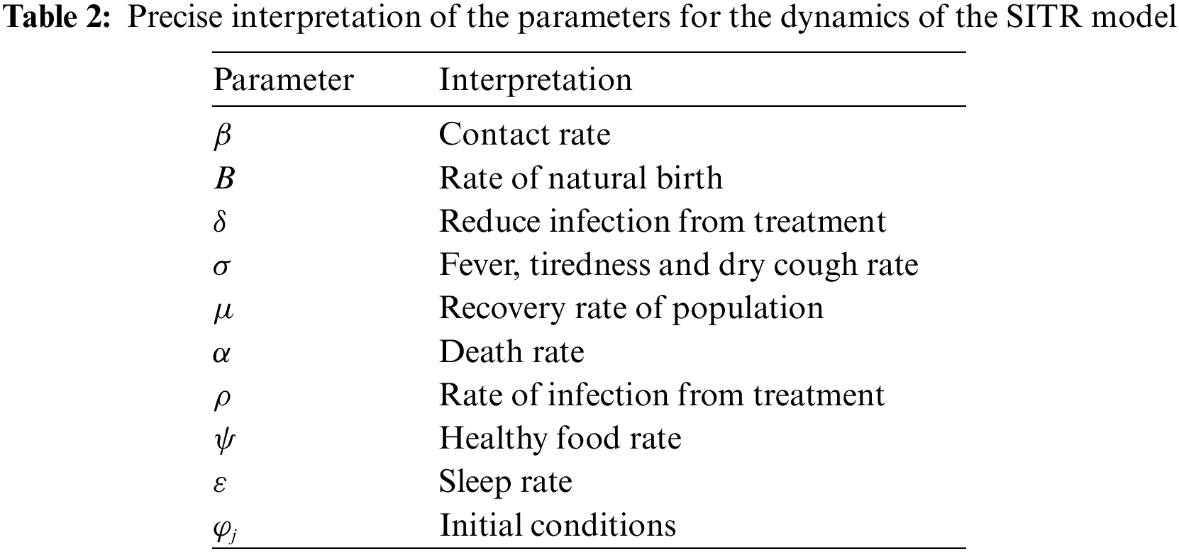
Each equation is describing the transmission behavior of individuals in the respective compartments. By this transmission number of individuals can vary in each of the five compartments [22–30]. The description of the transition rates in each cell is given in Table 2. The parameter of interest with appropriate settings for particular descriptions of the dynamics are provided in Tables 1 and 2.
We try to find the approximate solution of system of differential Eq. (1) with initial conditions as series of exponential functions. Exponential functions or exponential polynomials are based on the linearly independent exponential basis set
To begin with, we assume that the unique solutions of system (1) can be expressed as a exponential series of the form
then by truncation these power series after the
which, coefficients
Remark. We solve the system (Sys) in time interval [0, 1] and for larger intervals [0, R], convert it to interval [0, 1] by using an iterative method. This iterative process is such that to solve the system in
After solving these systems, we merge the functions as multivariate function.
3 Preliminaries and Matrix Relations
In this section, we outline operational matrices of the exponential method we will use in order to solve system (1).
In the first step, we create the differentiation matrices which are the basic tools of the current approach. Differentiation matrices make this method more suitable for managing high-order differential equations. By constructing an operational matrix, it is easy to derive high-order derivatives of the unknown in terms of values at collocation points.
Firstly, we inscribe the approximated solution
where
and
Taking advantage of the linearity of expansion (4), we can compute the derivative of u by differentiating the basic functions. The derivatives of u are obtained as follows:
and for higher order derivatives of u we present a matrix form. Next, we explain how to create a differentiation matrix through the method, and we extract and create a matrix
The derivative of the approximate solution can also be expressed as a product of matrices. Namely,
where the operational (differentiation) matrix
and that, after repeating the procedure k
holds for any nonnegative integer k, that
Note that
By using of the matrix relations (6) and (8), we can write matrix representation as
After replacing the collocation points
that, in the matrix form, we have
where
4 Implementation of Matrix Operation
In this section, we explain how to use the exponential collocation method for problem (1). For this purpose, we use the following procedure. The basis of this method is based on the calculation of unknown coefficients using the collocation points.
To acquire an exponential series solution of Eq. (1) under the conditions, the operational matrix method is applied as follows:
where
and
The relationship between
that by applying operational matrices, we obtain the following matrix forms:
Now let’s create the
where
and
The system (1) can be expressed as
that it can be rewritten as following matrix form:
where
and
To determine the unknown coefficients, we use the collocation points
and by replacing the collocation points into Eq. (15), we obtain a system of matrix equations as follows:
and this system corresponds to the following matrix form:
where
and
and
Now, let us find the relations between the matrix
After the substitution of the above relations, we obtain to the following matrix equation:
by previous definition
Briefly, (20) can also be presented as follows:
where
Here, (20) conforms to a nonlinear system of the
By placing the colocation points at the algebraic equations and considering initial conditions, the system be solved and the coefficients be determined.
Since most systems do not have exact solutions and most similar programs usually do not have the ability to generate numerical solutions, we must verify the accuracy of the numerical results using a method. We can confirm the accuracy and effectiveness of the numerical results by considering the residual error functions. The residual method is a general class of methods developed to obtain the approximate solution of differential equations. In the residual method, an approximate solution based on the overall behavior of the dependent variable is considered. The assumed solution is often chosen to satisfy the boundary conditions. This assumed solution is then replaced by the differential equation. Since the assumed solution is only approximate, it generally does not satisfy the differential equation and therefore leads to an error or what we call the residual. The residual then disappears in the mean sense throughout the solution domain to produce a system of algebraic equations.
If
The rate of increase in the number of infections depends on the product of the number of infected and susceptible persons. The system (1) explains the dramatic increase in infection rates worldwide. The travel of infected individuals around the world has led to an increase in the number of infected people, which in turn has led to a further increase in the susceptible individuals. This creates a positive feedback loop that leads to a rapid increase in the number of actively infected persons. Therefore, during the period of increase, the number of susceptible people increases and consequently the number of infected people also increases.
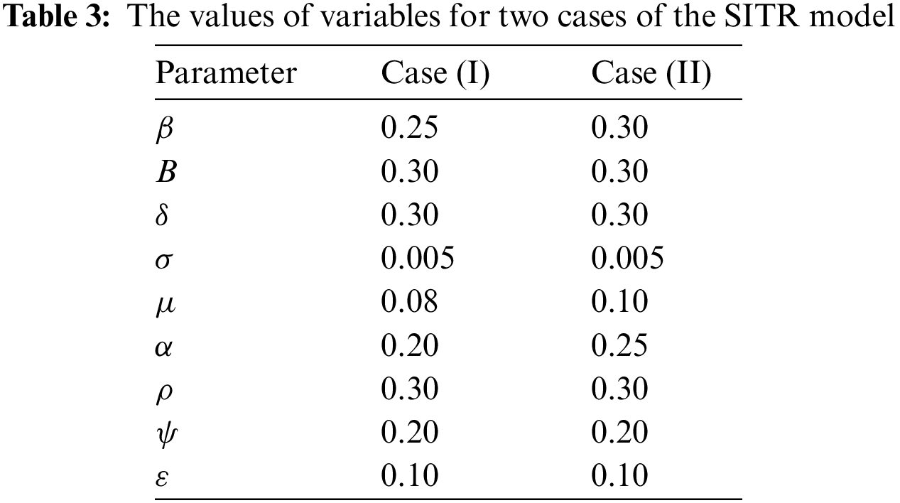
In this section, we present some applications of the method that are presented in different values for the parameters
Case (I):
Case (II):
These results show the effectiveness of the present method in achieving good accuracy with fewer collocation points and less computational time. All the calculations have been performed using MAPLE. By applying the suggested method for
The residual of solutions has been used to show that this method is efficient and reasonably accurate.
The coefficients of the approximate numerical outcomes of the method for
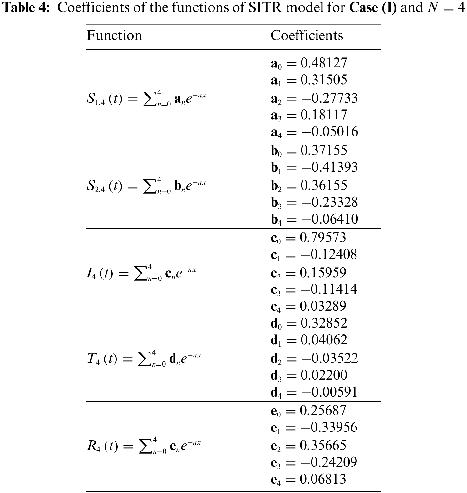
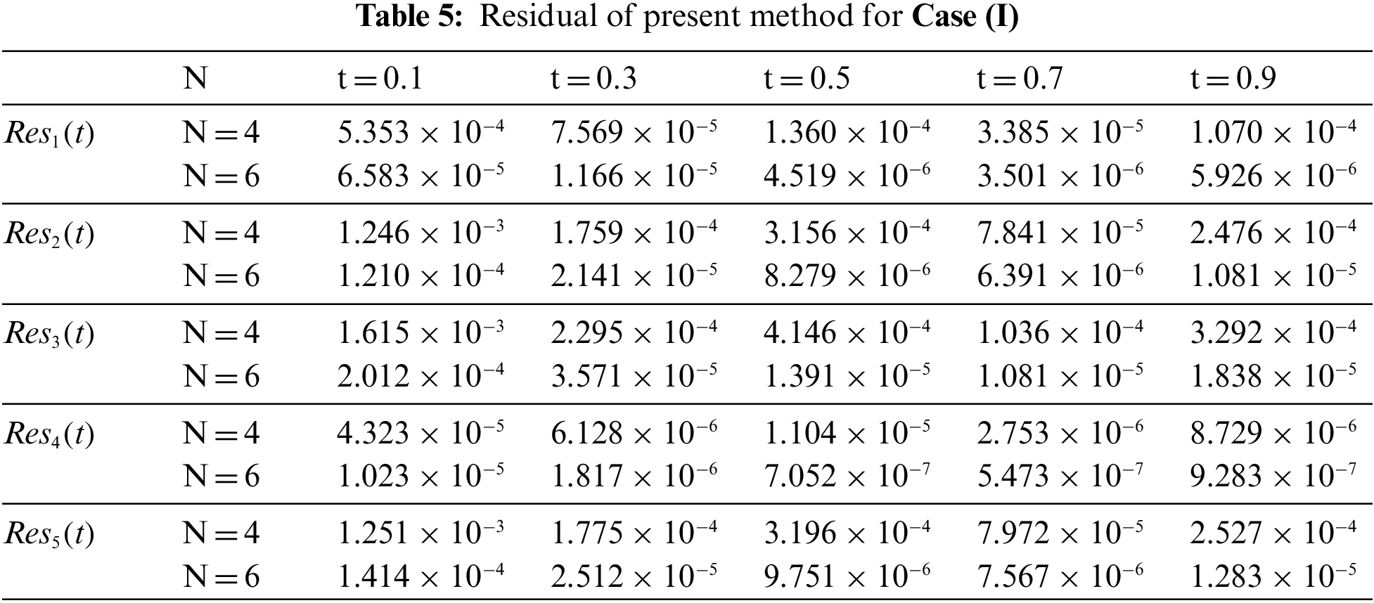
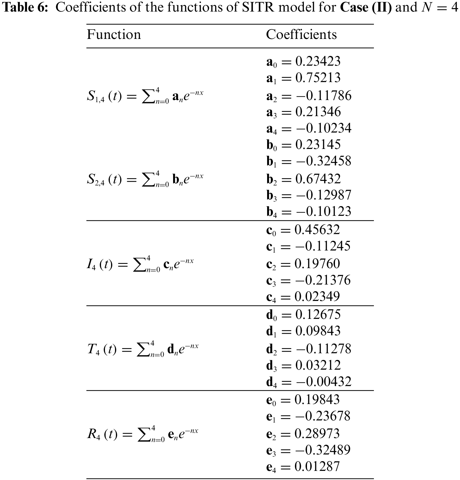
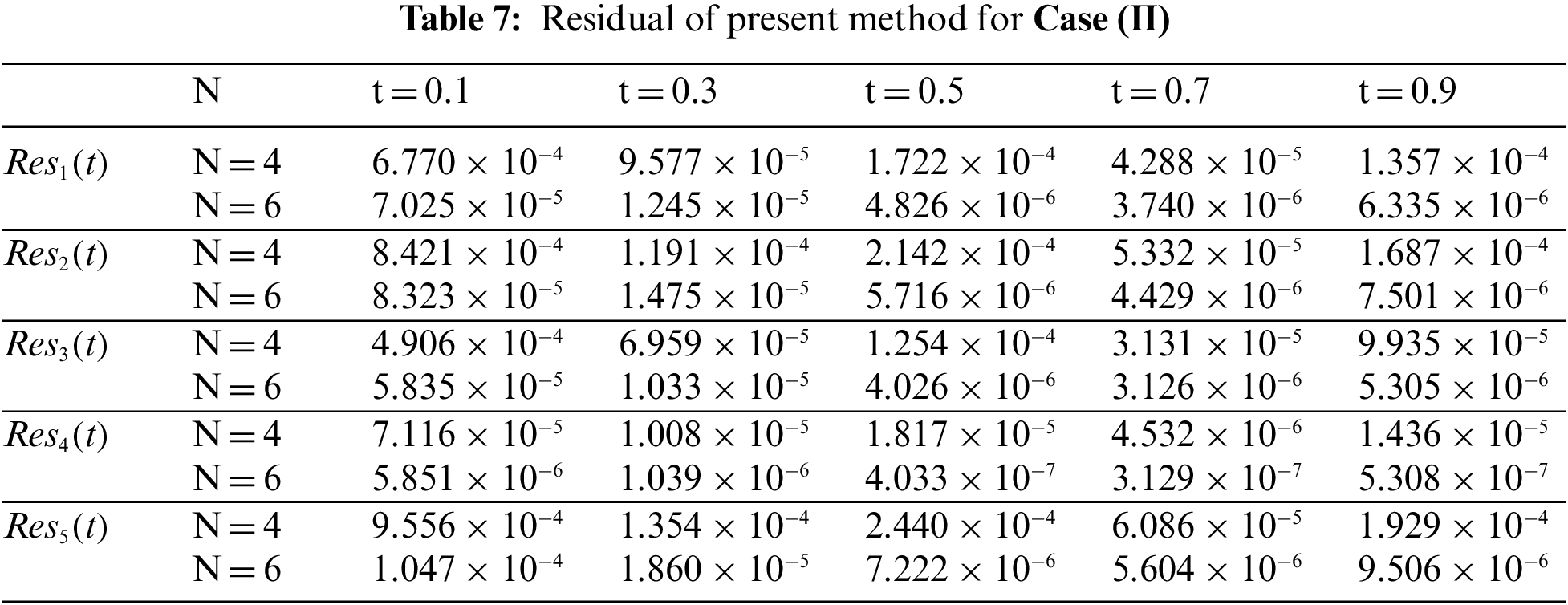
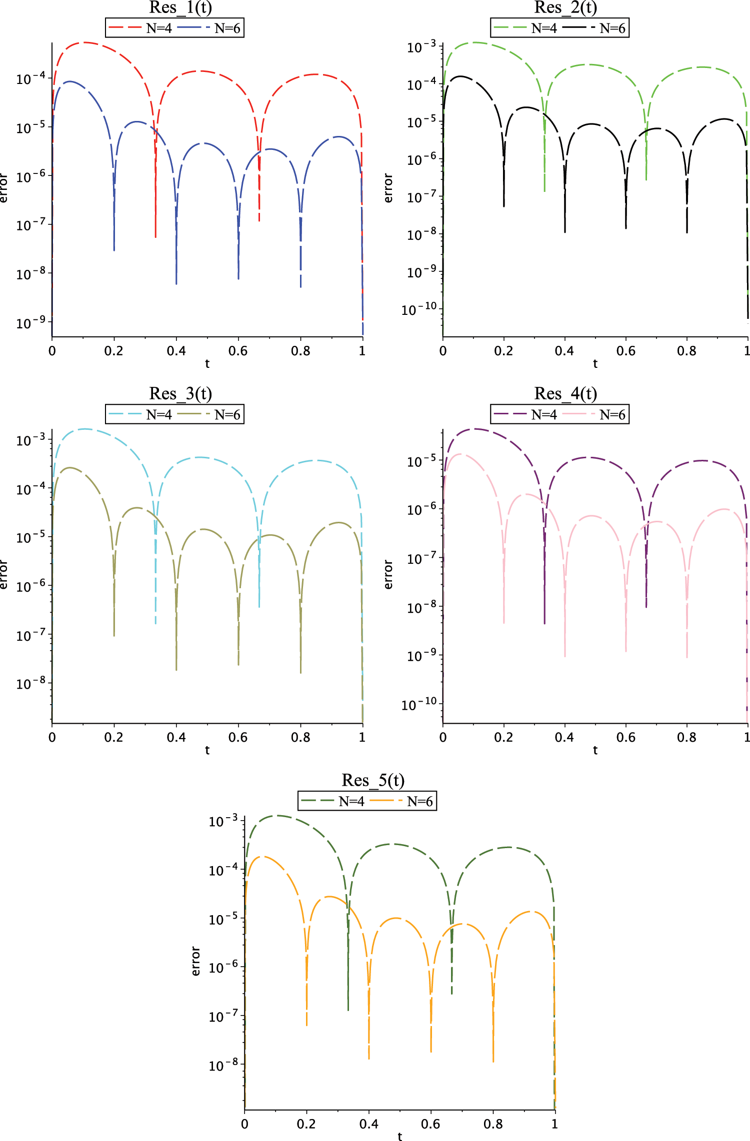
Figure 1: Graph of residual errors for Case (I) for
In Fig. 2, graph of functions
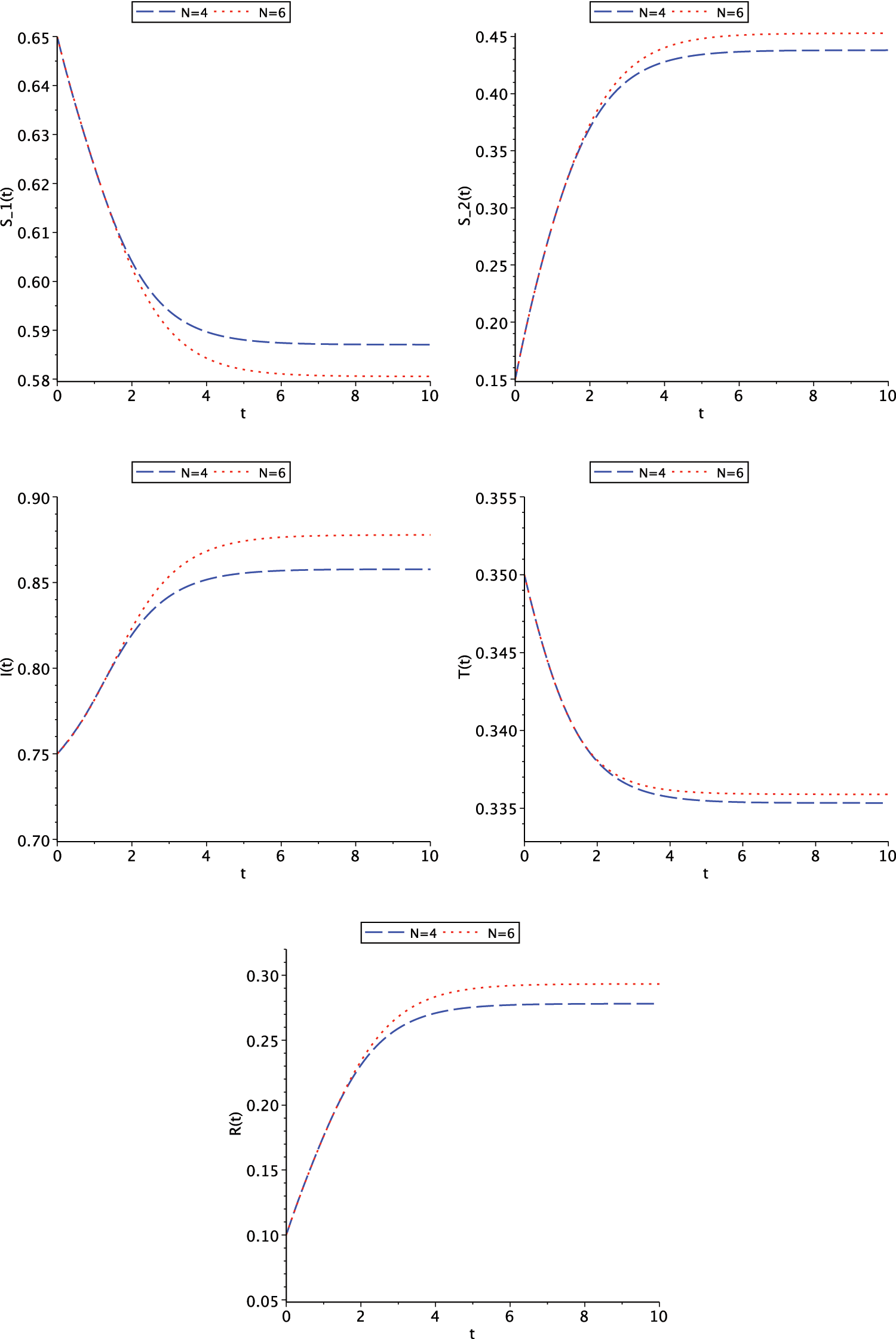
Figure 2: Graph of functions
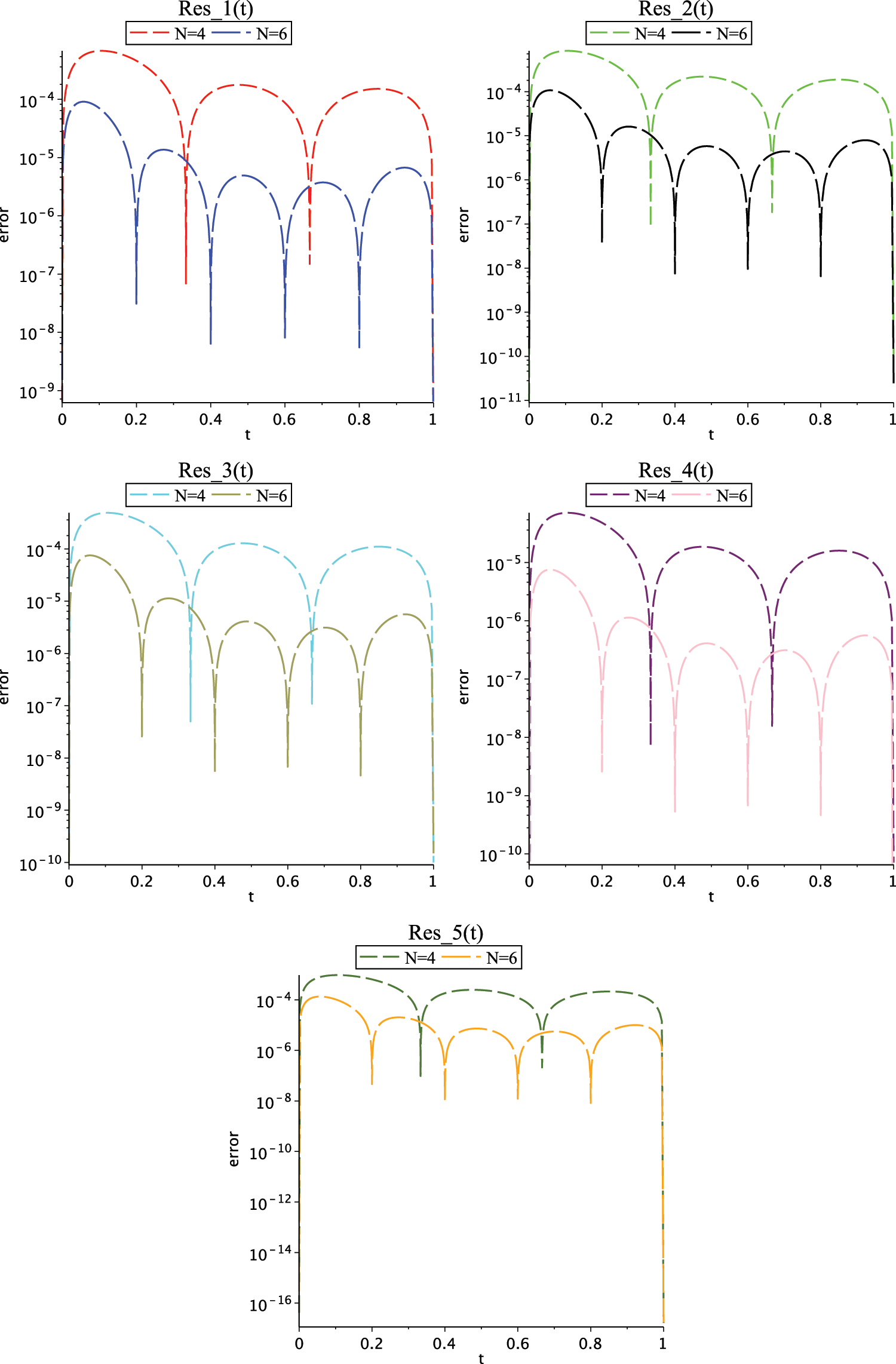
Figure 3: Graph of residual errors for Case (II) for
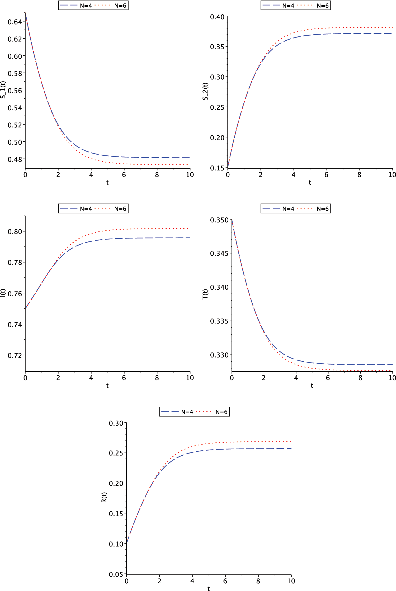
Figure 4: Graph of functions
These graphs show that contact rates are primarily a source of large increase in the number of susceptible individuals, but begin to decrease over time. This is because higher contact rates cause more people to become infected and move to an infected class; therefore, the number of individuals in the susceptible class decreases. About
The figures also show that with a high death rate, the number of recovered individuals suddenly decreases. Because when the death rate is high, so many people in the affected and recovered classes lose their lives, resulting in a decrease in people in all the classes. Since the death rate is so high, the infected and recovered people are almost gone.
Figs. 5 and 6 show the graph of residual error functions for Case (I) and Case (II) on interval
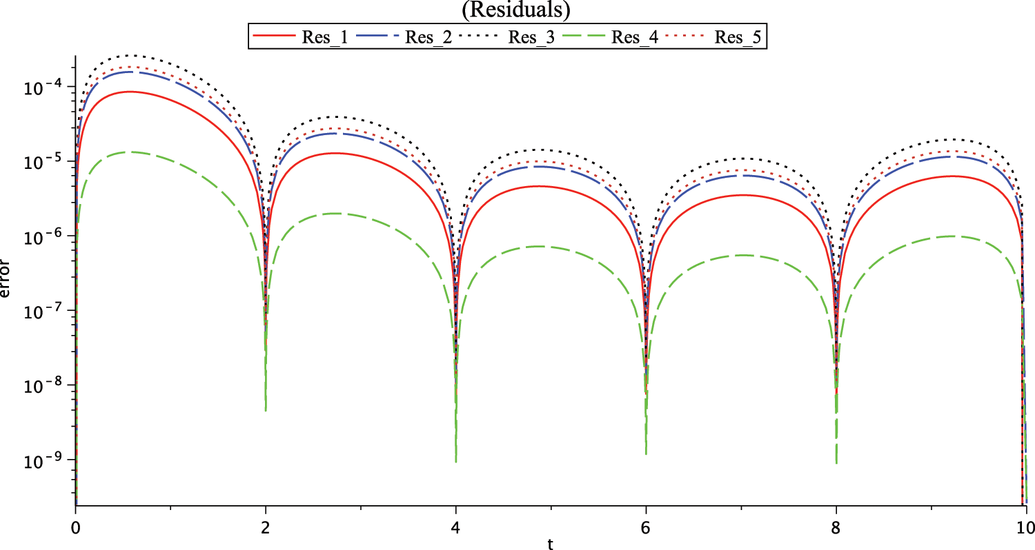
Figure 5: Graph of residuals for Case (I),
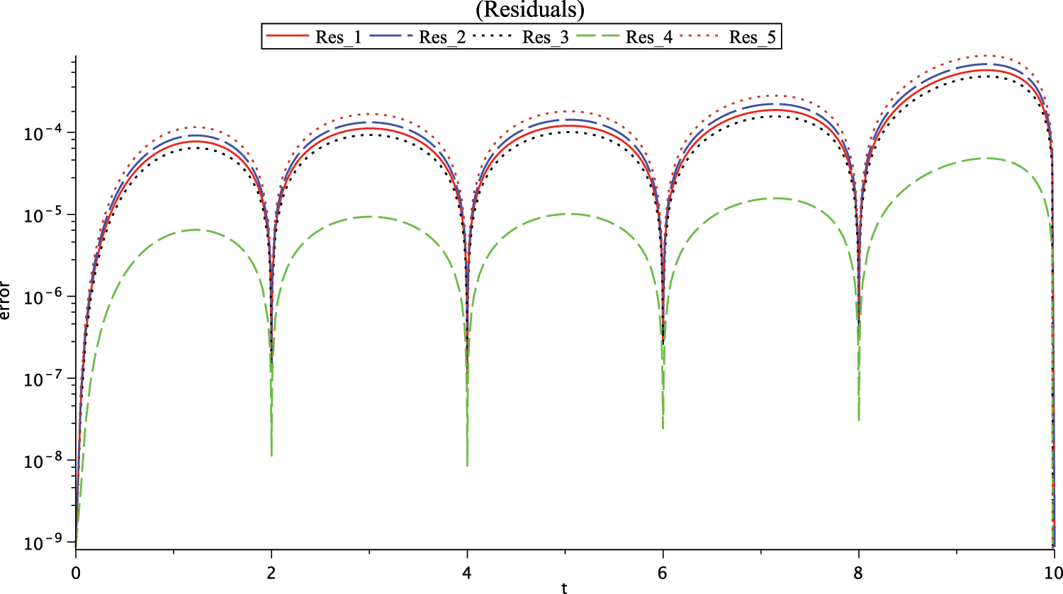
Figure 6: Graph of residual errors for Case (II)
In this paper, the exponential approximation is used to solve the numerical investigation of a nonlinear SITR model that represents the dynamics of the new disease of COVID-19. The method is based on exponential functions and the collocation method as an operational matrix. As seen, there is no concern about approximating higher-order derivatives of the unknowns. Also, to show the accuracy and efficiency of the method, two cases with different values have been examined. Through the examples provided, we realize that the obtained numerical results have very good residual errors. Moreover, it is realized that errors decrease when N values increase. As shown in the results obtained from computations, we conclude that implementation of this method will be very easy with less computational costs for similar problems. The results indicate the effectiveness of the present method in achieving good accuracy with fewer collocation points and less computational time.
Acknowledgement: The authors wish to express their appreciation to the reviewers for their helpful suggestions which greatly improved the presentation of this paper.
Funding Statement: The authors received no specific funding for this study.
Conflicts of Interest: The authors declare that they have no conflicts of interest to report regarding the present study.
References
1. Ndaïrou, F., Area, I., Nieto, J. J., Torres, D. F. M. (2020). Mathematical modeling of COVID-19 transmission dynamics with a case study of Wuhan. Chaos, Solitons and Fractals, 135, 109846. DOI 10.1016/j.chaos.2020.109846. [Google Scholar] [CrossRef]
2. Olumuyiwa, J. P., Qureshi, S., Yusuf, A., Al-Shomrani, M., Idowu, A. A. (2021). A new mathematical model of COVID-19 using real data from Pakistan. Results in Physics, 24, 104098. DOI 10.1016/j.rinp.2021.104098. [Google Scholar] [CrossRef]
3. Farman, M., Akgul, A., Ahmad, A., Baleanu, D., Saleem, M. U. (2021). Dynamical transmission of coronavirus model with analysis and simulation. Computer Modeling in Engineering & Sciences, 127(2), 753–769. DOI 10.32604/cmes.2021.014882. [Google Scholar] [CrossRef]
4. Iqbal, S., Baleanu, D., Ali, J., Younas, H. M., Riaz, M. B. (2021). Fractional analysis of dynamical novel COVID-19 by semi-analytical technique. Computer Modeling in Engineering & Sciences, 129(2), 705–727. DOI 10.32604/cmes.2021.015375. [Google Scholar] [CrossRef]
5. Sabir, Z., Alnahdi, A. S., Jeelani, M. B., Abdelkawy, M. A., Asif, M. et al. (2022). Numerical computational heuristic through morlet wavelet neural network for solving the dynamics of nonlinear SITR COVID-19. Computer Modeling in Engineering & Sciences, 131(2), 763–785. DOI 10.32604/cmes.2022.018496. [Google Scholar] [CrossRef]
6. Hoehl, S., Rabenau, H., Annemarie, B., Kortenbusch, M., Cinatl, J. et al. (2020). Evidence of SARS-CoV-2 infection in returning travelers from Wuhan, China. New England Journal of Medicine, 382, 1278–1280. DOI 10.1056/NEJMc2001899. [Google Scholar] [CrossRef]
7. Chen, T. M., Rui, J., Wang, Q. P. (2020). A mathematical model for simulating the phase-based transmissibility of a novel coronavirus. Infectious Diseases of Poverty, 9, 24. DOI 10.1186/s40249-020-00640-3. [Google Scholar] [CrossRef]
8. Wai-Kit, M., Huang, J., Zhang, C. J. P. (2020). Breaking down of the healthcare system: Mathematical modelling for controlling the novel coronavirus (2019-nCoV) outbreak in Wuhan, China. bioRxiv, 1–21. [Google Scholar]
9. Anwar, Z., Alzahrani, E., Erturk, V. S., Zaman, G. (2020). Mathematical model for coronavirus disease 2019 (COVID-19) containing isolation class. BioMed Research International, 2020, 3452402. [Google Scholar]
10. Umar, M., Sabir, Z., Raja, M. A. Z., Shoaib, M., Gupta, M. et al. (2020). A stochastic intelligent computing with neuro-evolution heuristics for nonlinear SITR system of novel COVID-19 dynamics. Symmetry, 12, 1628. DOI 10.3390/sym12101628. [Google Scholar] [CrossRef]
11. Khan, M. A., Atangana, A. (2020). Modeling the dynamics of novel coronavirus (2019-nCoV) with fractional derivative. Alexandria Engineering Journal, 59, 2379–2389. DOI 10.1016/j.aej.2020.02.033. [Google Scholar] [CrossRef]
12. Sanchez, Y. G., Sabir, Z., Guirao, J. L. (2020). Design of a nonlinear sitr fractal model based on the dynamics of a novel coronavirus (COVID-19). Fractals, 28, 2040026. DOI 10.1142/S0218348X20400265. [Google Scholar] [CrossRef]
13. Yüzbaşi, S. (2016). An exponential collocation method for the solutions of the HIV infection model of CD4+ T cells. International Journal of Biomathematics, 9, 165003. [Google Scholar]
14. Shivanian, E., Aslefallah, M. (2017). Stability and convergence of spectral radial point interpolation method locally applied on two-dimensional pseudo-parabolic equation. Numerical Methods for Partial Differential Equations, 33, 724–741. DOI 10.1002/num.22119. [Google Scholar] [CrossRef]
15. Aslefallah, M., Shivanian, E. (2015). Nonlinear fractional integro-differential reaction-diffusion equation via radial basis functions. The European Physical Journal Plus, 130, 1–9. [Google Scholar]
16. Aslefallah, M., Abbasbandy, S., Shivanian, E. (2020). Meshless singular boundary method for two dimensional pseudo-parabolic equation: Analysis of stability and convergence. Journal of Applied Mathematics and Computing, 63, 585–606. DOI 10.1007/s12190-020-01330-x. [Google Scholar] [CrossRef]
17. Aslefallah, M., Abbasbandy, S., Shivanian, E. (2019). Numerical solution of a modified anomalous diffusion equation with nonlinear source term through meshless singular boundary method. Engineering Analysis with Boundary Elements, 107, 198–207. DOI 10.1016/j.enganabound.2019.07.016. [Google Scholar] [CrossRef]
18. Yüzbaşi, S., Sezer, M. (2013). An exponential approximation for solutions of generalized pantograph-delay differential equations. Applied Mathematical Modelling, 37, 9160–9173. DOI 10.1016/j.apm.2013.04.028. [Google Scholar] [CrossRef]
19. Yüzbaşi, S. (2020). An operational method for solutions of riccati type differential equations with functional arguments. Journal of Taibah University for Science, 14, 661–669. DOI 10.1080/16583655.2020.1761661. [Google Scholar] [CrossRef]
20. Yüzbaşi, S. (2018). An exponential method to solve linear Fredholm-Volterra integro-differential equations and residual improvement. Turkish Journal of Mathematics, 42(5), 2546–2562. DOI 10.3906/mat-1707-66. [Google Scholar] [CrossRef]
21. Yüzbaşi, S., Sezer, M. (2013). An exponential matrix method for numerical solutions of Hantavirus infection model. Applications and Applied Mathematics, 8, 99–115. [Google Scholar]
22. Sene, N. (2022). Fundamental results about the fractional integro-differential equation described with caputo derivative. Journal of Function Spaces, 2022, 9174488. DOI 10.1155/2022/9174488. [Google Scholar] [CrossRef]
23. Sene, N. (2022). 2-numerical methods applied to a class of SEIR epidemic models described by the caputo derivative. Methods of Mathematical Modeling, 2022, 23–40. DOI 10.1016/B978-0-323-99888-8.00003-6. [Google Scholar] [CrossRef]
24. Ahmad, A., Farman, M., Ghafar, A., Inc, M., Ahmad, M. O. et al. (2022). Analysis and simulation of fractional order smoking epidemic model. Computational and Mathematical Methods in Medicine, 2022, 1–16. DOI 10.1155/2022/9683187. [Google Scholar] [CrossRef]
25. Devi, S. A., Felix, A., Narayanamoorthy, S., Ahmadian, A., Balaenu, D. et al. (2022). An intuitionistic fuzzy decision support system for COVID-19 lockdown relaxation protocols in India. Computers and Electrical Engineering, 101, 108–166. [Google Scholar]
26. Geetha, S., Narayanamoorthy, S., Manirathinam, T., Ahmadian, A., Bajuri, M. Y. et al. (2022). Knowledge-based normative safety measure approach: Systematic assessment of capabilities to conquer COVID-19. The European Physical Journal Special Topics, 2022, 1–13. DOI 10.1140/epjs/s11734-022-00617-3. [Google Scholar] [CrossRef]
27. Ali, M. R., Sadat, R. (2021). Lie symmetry analysis, new group invariant for the (3 + 1)-dimensional and variable coefficients for liquids with gas bubbles models. Chinese Journal of Physics, 71, 539–547. DOI 10.1016/j.cjph.2021.03.018. [Google Scholar] [CrossRef]
28. Ali, M. R., Sadat, R. (2021). Construction of lump and optical solitons solutions for (3 + 1) model for the propagation of nonlinear dispersive waves in inhomogeneous media. Optical and Quantum Electronics, 53(6), 279. DOI 10.1007/s11082-021-02916-w. [Google Scholar] [CrossRef]
29. Ozkose, F., Yavuz, M. (2022). Investigation of interactions between COVID-19 and diabetes with hereditary traits using real data: A case study in Turkey. Computers in Biology and Medicine, 141(3), 105044. [Google Scholar]
30. Naik, P. A., Zu, J., Ghori, M. B., Naik, M. (2021). Modeling the effects of the contaminated environments on COVID-19 transmission in India. Results in Physics, 29, 104774. DOI 10.1016/j.rinp.2021.104774. [Google Scholar] [CrossRef]
Cite This Article
 Copyright © 2023 The Author(s). Published by Tech Science Press.
This work is licensed under a Creative Commons Attribution 4.0 International License , which permits unrestricted use, distribution, and reproduction in any medium, provided the original work is properly cited.
 Downloads
 Citation Tools