
 Submit a Paper
 Propose a Special lssue
 Open Access
ARTICLE

Effect of Measurement Error on the Multivariate CUSUM Control Chart for Compositional Data
1 School of Automation, Nanjing University of Science and Technology, Nanjing, 210094, China
2 School of Economics and Statistics, Guangzhou University, Guangzhou, 510006, China
3 Department of Mathematics and Statistics, East China Normal University, Shanghai, 200062, China
4 Department of Statistics, Government Ambala Muslim Graduate College, Sargodha, 40100, Pakistan
5 Department of Statistics, University of Sargodha, Sargodha, 40100, Pakistan
* Corresponding Author: Jinsheng Sun. Email:
Computer Modeling in Engineering & Sciences 2023, 136(2), 1207-1257. https://doi.org/10.32604/cmes.2023.025492
Received 16 July 2022; Accepted 27 September 2022; Issue published 06 February 2023
 View Full Text
 Download PDF
Abstract
Control charts (CCs) are one of the main tools in Statistical Process Control that have been widely adopted in manufacturing sectors as an effective strategy for malfunction detection throughout the previous decades. Measurement errors (M.E’s) are involved in the quality characteristic of interest, which can effect the CC’s performance. The authors explored the impact of a linear model with additive covariate M.E on the multivariate cumulative sum (CUSUM) CC for a specific kind of data known as compositional data (CoDa). The average run length is used to assess the performance of the proposed chart. The results indicate that M.E’s significantly affects the multivariate CUSUM-CoDa CCs. The authors have used the Markov chain method to study the impact of different involved parameters using six different cases for the variance-covariance matrix (VCM) (i.e., uncorrelated with equal variances, uncorrelated with unequal variances, positively correlated with equal variances, positively correlated with unequal variances, negatively correlated with equal variances and negatively correlated with unequal variances). The authors concluded that the error VCM has a negative impact on the performance of the multivariate CUSUM-CoDa CC, as the increases with an increase in the value of the error VCM. The subgroup size m and powering operator b positively impact the proposed CC, as the decreases with an increase in m or b. The number of variables p also has a negative impact on the performance of the proposed CC, as the values of increase with an increase in p. For the implementation of the proposal, two illustrated examples have been reported for multivariate CUSUM-CoDa CCs in the presence of M.E’s. One deals with the manufacturing process of uncoated aspirin tablets, and the other is based on monitoring the machines involved in the muesli manufacturing process.Keywords
A widely used method is statistical process control (SPC) to monitor a process. SPC is a decision-making tool used in almost all industrial manufacturing processes to achieve process stability and sustainable quality product. W. A. Shewhart introduced the CCs in the 1920s. The goal of a CC is to find assignable causes of shifts and to minimize the production of a large number of defective items. In practice, determining which CC is appropriate for specific data can be difficult. It is possible to figure out by looking at the distribution of the underlying data process. CCs with compound or simple rules can be computed using the run-length distribution using a Markov chain approach [1]. Based on concomitant order statistics and long-run dependence, a new bivariate semiparametric CC is proposed by Koutras et al. [2]. Integrating techniques for preventive maintenance and quality control policies with the time-between-event chart for reliability-oriented design has been investigated by He et al. [3]. Recently under different classical estimators, control charts for shape parameters of power function distributions were studied by Zaka et al. [4]. Hybrid EWMA CCs are designed to monitor process dispersion efficiently for the automotive industry [5]. For trimethylchlorosilane purification, simulations and multivariate CCs are utilized to increase the effectiveness [6].
Multivariate EWMA CCs are proposed using multiple variables based on an AIC calculation for multivariate SPC [7]. The frequency of unblinded and blinded adverse events accumulating from single and multiple trials using CCs was monitored in [8]. The
Compositional data (CoDa) vectors are positive components presented as percentages, ratios, proportions or parts of a whole. Aitchison’s principles and statistical tools from [13] have been used to solve many practical problems. For more information about CoDa, readers are referred to [14] and [15]. Because the CoDa variable aggregates are limited to constant values, they can not be used the same way as standard multivariate data [16]. CoDa has applications in various fields, including chemical research surveys, geology, engineering sciences and econometric data analysis. Some of the most recent articles dealing with statistical methods and CoDa processing are discussed here. An automobile market application in which the authors model brand share of the market as a function of media investments while taking account of the brand’s cost using CoDa regression has been examined [17]. The sample space’s algebraic-geometric structure was introduced to adhere to the principles of sample space and the structure of CoDa [18]. Recently, Zaidi et al. [19] investigated the impact of M.E’s on Hotelling
The CUSUM charts are well-known for detecting smaller and more frequent changes than Shewhart charts and are among the most common and widely used charts in practice [22]. Risk monitoring for CUSUM CCs with model error suggested by Knoth et al. [23]. Further, Shu et al. [24] analyzed the CUSUM accounting process for monotone population changes. It is essential to optimize several multiple objective functions simultaneously when performing multi-objective optimization and the multivariate CC method is unaffected by small and moderate variable shifts [25]. Such multivariate charts are commonly used to detect changes in process parameters around their corresponding axes, which must be illustrated in a specific direction. The MCUSUM charts for detecting shifts in MV and VCM have been discussed in [26]. A double progressive mean CC for monitoring Poisson process observations has been discussed in [27]. Furthermore, Alevizakos et al. [28] proposed a triple moving average CC to improve the chart’s detection ability and found them to be more effective than the moving average and double moving average CCs in detecting small to moderate shifts.
CCs are often created with the hypothesis that the factor of the quality feature is assessed accurately. However, M.E’s can occur due to various circumstances. Many researchers examined the impact of M.E’s on CCs. Imprecise measurement instruments or human errors are two main causes contributing to M.E’s. The presence of M.E’s must be taken into account while implementing CCs because it has a huge impact on their performance [29]. A cumulative sum (CUSUM) CCs has been proposed for the drilling process to monitor the variations of discharge pulses for sensing the actual condition of the whole drilling process taking M.E’s into account [30]. For a finite horizon production process, Nguyen et al. [31] suggested one-sided Shewhart-type and EWMA
Typically, practitioners monitor processes without considering the possibility of M.E’s. Despite sophisticated measurement techniques and methodologies, M.E’s is commonly caused by operational and environmental factors. As Montgomery et al. [34] outlined, Gage capacity tests commonly quantify M.E’s variability. The impacts of M.E’s on the functionality of a multivariate CC for the combined monitoring of normal processes MV and VCM have been studied by Maleki et al. [35]. A thorough examination of the impact of M.E’s in SPC has been conducted by Maravelakis et al. [36]. The performance analysis of univariate adaptive CCs in the existence of M.E’s has been examined by Hu et al. [37]. Based on an additive covariate model, Maleki et al. [38] investigated the adverse effects of M.E’s on the detection performance of triple sampling
Although many studies on the assessment of CCs in the presence of M.E’s have been conducted, few have focused on multivariate data, and very few researchers have contributed to CoDa. But as far as the authors are aware, none of them has been dedicated to MCUSUM CC for
A row vector
where
As CoDa deals with the constraint of constant sum, Euclidean geometry is not supposed to be useful for CoDa. Let us take an example to make it more clear, Suppose there are two CoDa vectors,
• the perturbation operator
• the powering operator
The constant sum constraint makes CoDa difficult to deal with in its original form, hence pre-defined log-ratio transformations (LRT) can be used to transform CoDa from
where
Another LRT for a CoDa vector
where for
Also, there is inverse ILRT, which can transform the
In this paper, the CoDa vectors are denoted without a “*” sign, while the transformed vectors are denoted with a “*” in the superscript.
3 Additive Measurement Errors Model for CoDa
Assume that there are p-part compositions
where
where
One can refer to Appendix A for the estimation of
4 Multivariate CUSUM CC for Compositional Data
Assume we have
where
with
The MCUSUM-CoDa CC displays a signal when
To assess the MCUSUM-CoDa CC’s run-length efficiency, the authors implement a Markov chain approximation suggested by Crosier [42]. The Markov Chain model needed to measure the MCUSUM-CoDa chart’s
Lowry et al. [44] proposed
When M.E’s is included in the process, the non-centrality parameter is denoted by
Linna et al. [32] examined the effectiveness of the shift detection of multivariate charts and found them to be more effective in detecting a shift in one direction and ineffective in detecting a shift in the other direction. For this reason, Linna et al. [32] proposed using the minimum and maximum values of
where
The
The authors assumed the unit sample size
5 Performance Evaluation of the MCUSUM-CoDa CC in the Presence of M.E’s
This section aims to evaluate the performance of the MCUSUM-CoDa CC in the presence of M.E’s. The M.E’s VCM equals
• Select the most appropriate value for the
• Select a particular value of k. In this case, following [46], we choose
• Obtain the value of H such that
• Select the optimal value of H* from all the H values such that the
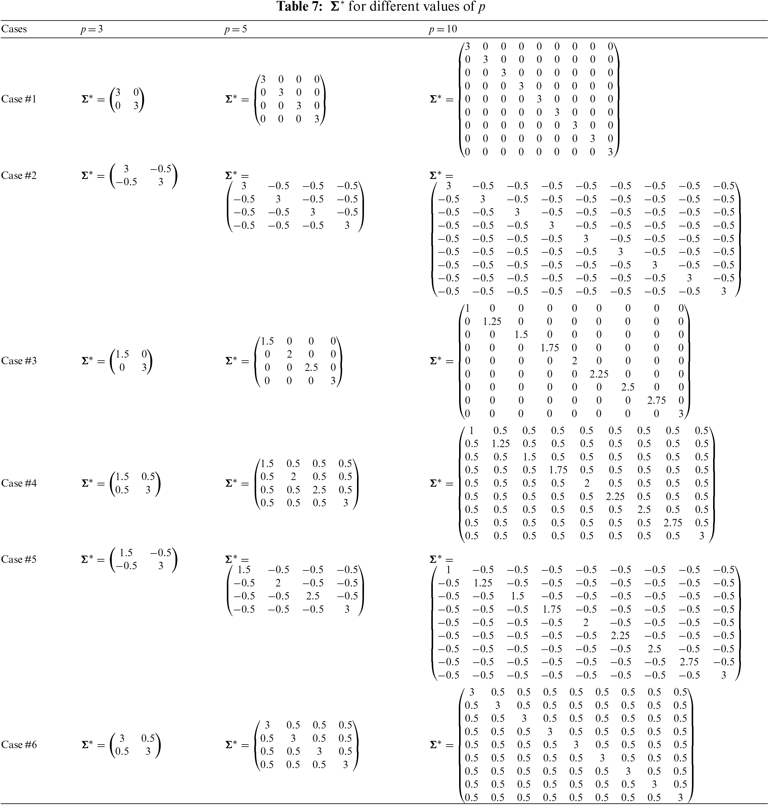
The following six cases for the CoDa VCM
Case #I uncorrelated with equal variances
Case #II negatively correlated with equal variances
Case #III uncorrelated with unequal variances
Case #IV positively correlated with unequal variances
Case #V negatively correlated with unequal variances
Case #VI positively correlated with equal variances
The goal is to investigate the effect of involved parameters
This subsection investigates the effect of the involved parameters
• The M.E VCM
• The subgroup size m has a positive impact on the
• The powering constant b has a positive impact on the
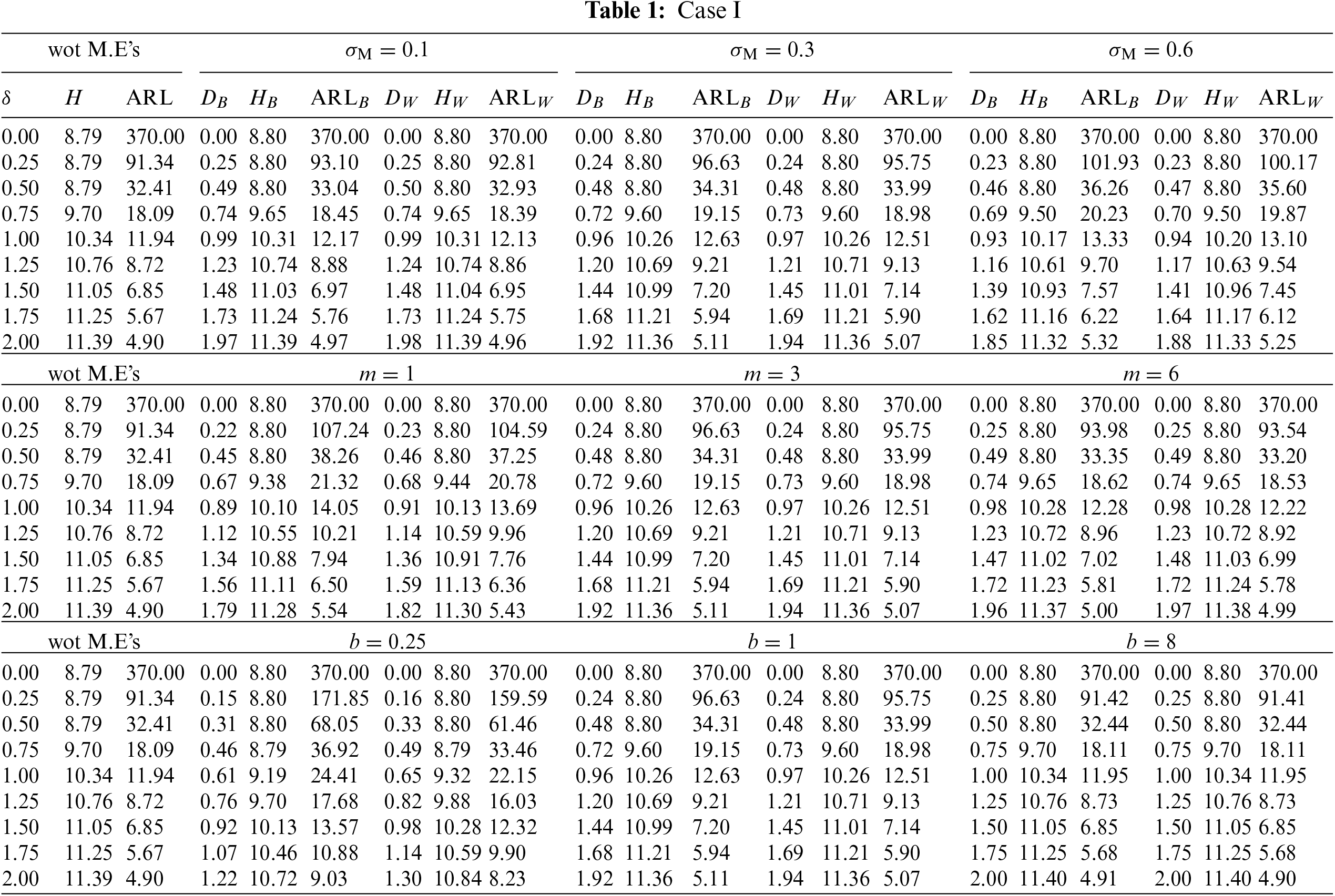

Figure 1:
This subsection investigates the effect of the involved parameters
• The M.E VCM
• The subgroup size m has a positive impact on the
• The powering constant b has a positive impact on the
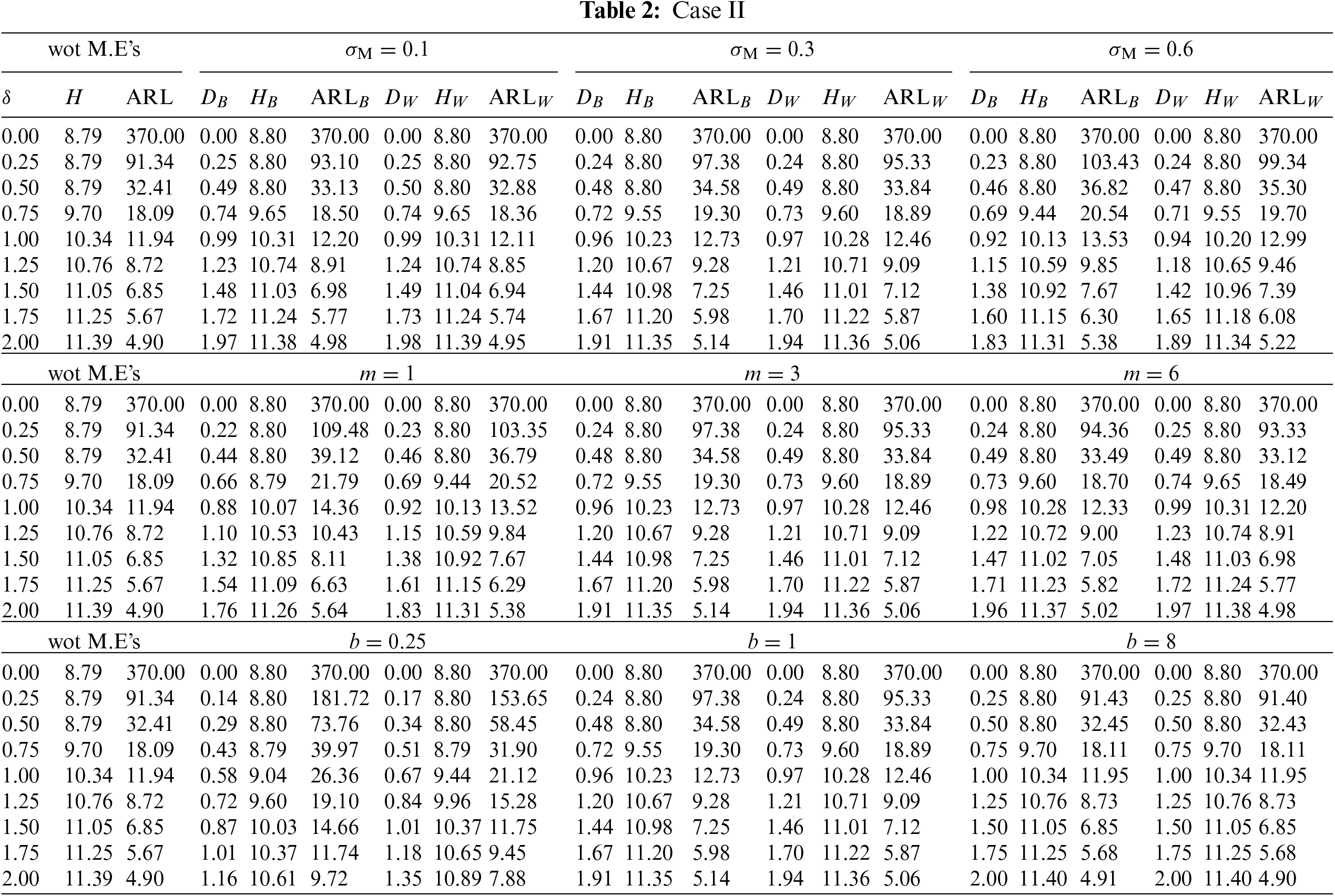
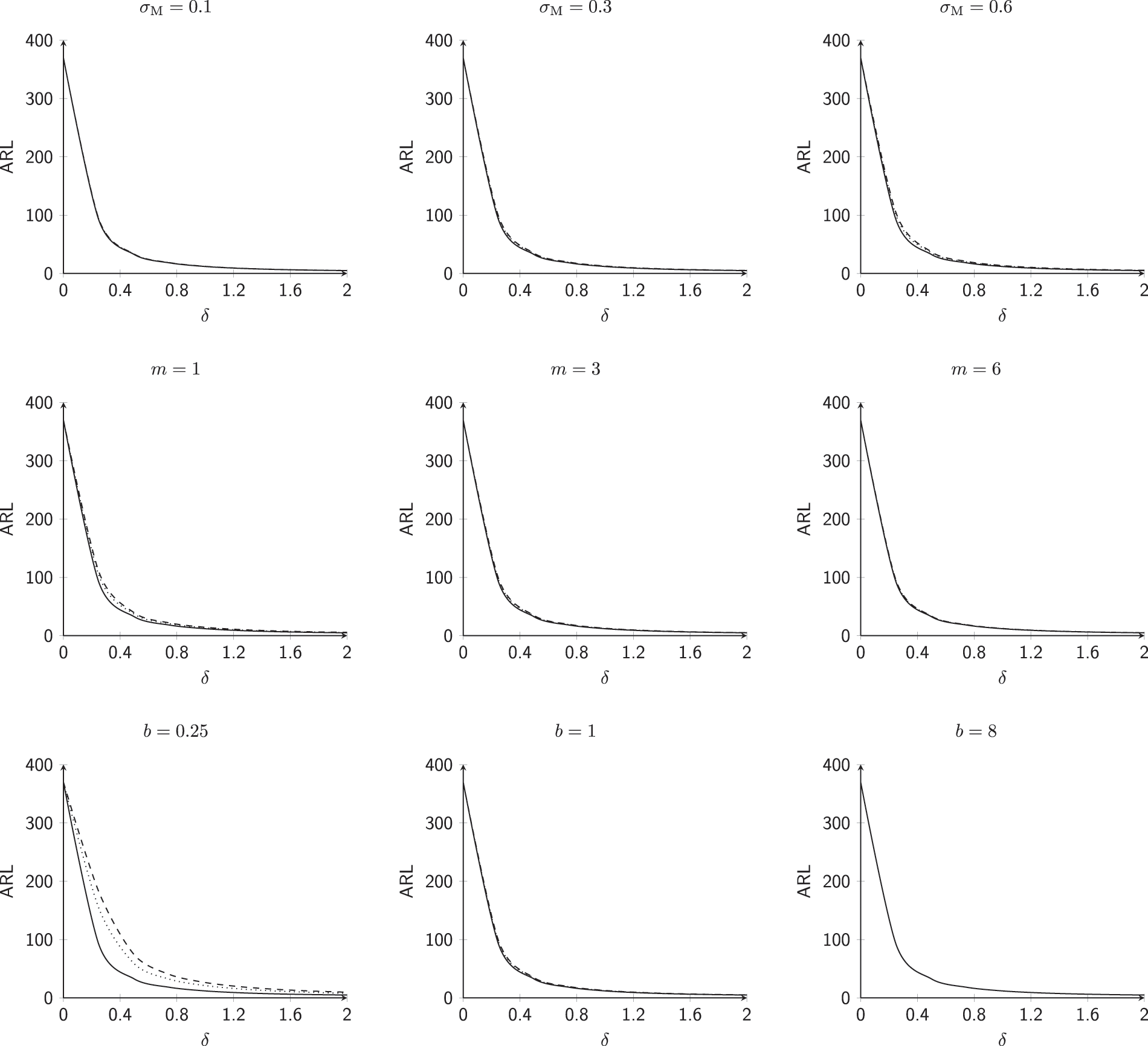
Figure 2:
This subsection investigates the effect of the involved parameters
• The M.E VCM
• The subgroup size m has a positive impact on the
• The powering constant b has a positive impact on the
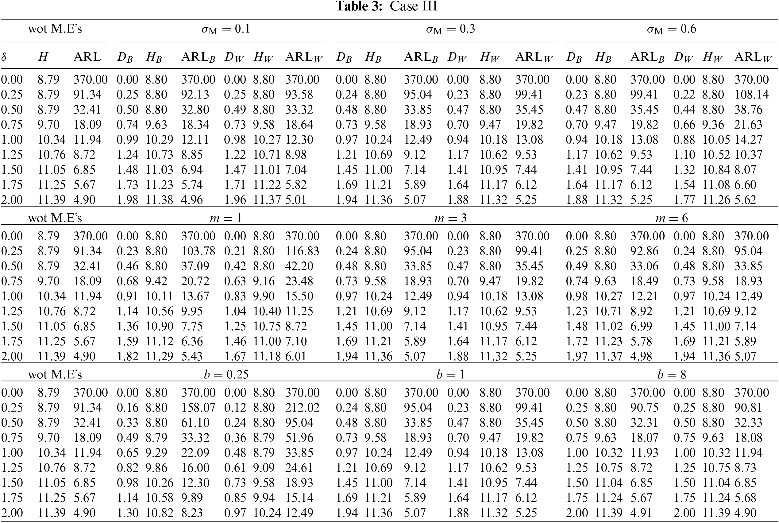

Figure 3:
This subsection investigates the effect of the involved parameters
• The M.E VCM
• The subgroup size m has a positive impact on the
• The powering constant b has a positive impact on the
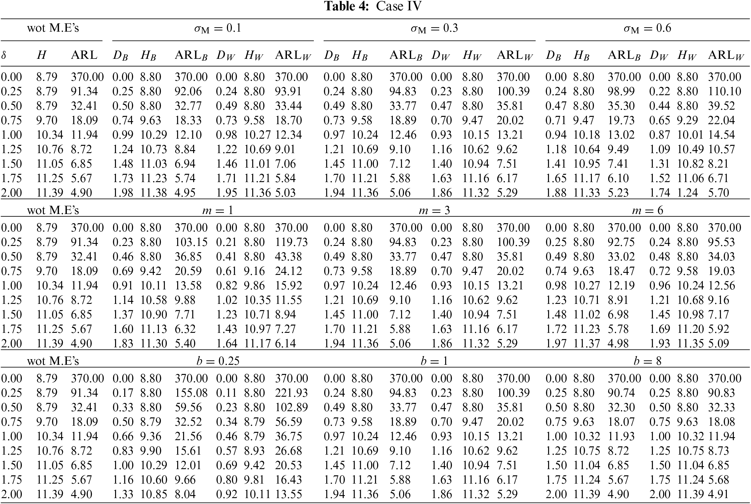

Figure 4:
This subsection investigates the effect of the involved parameters
• The
• The M.E VCM
• The subgroup size m has a positive impact on the
• The powering constant b has a positive impact on the
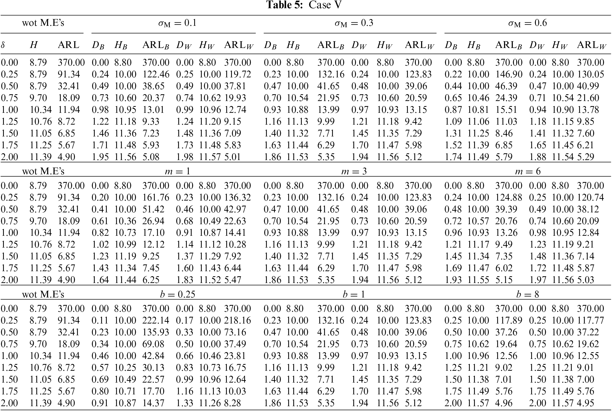

Figure 5:
This subsection investigates the effect of the involved parameters
• Similar to Case #5, the
• The M.E VCM
• The subgroup size m has a positive impact on the
• The powering constant b has a positive impact on the
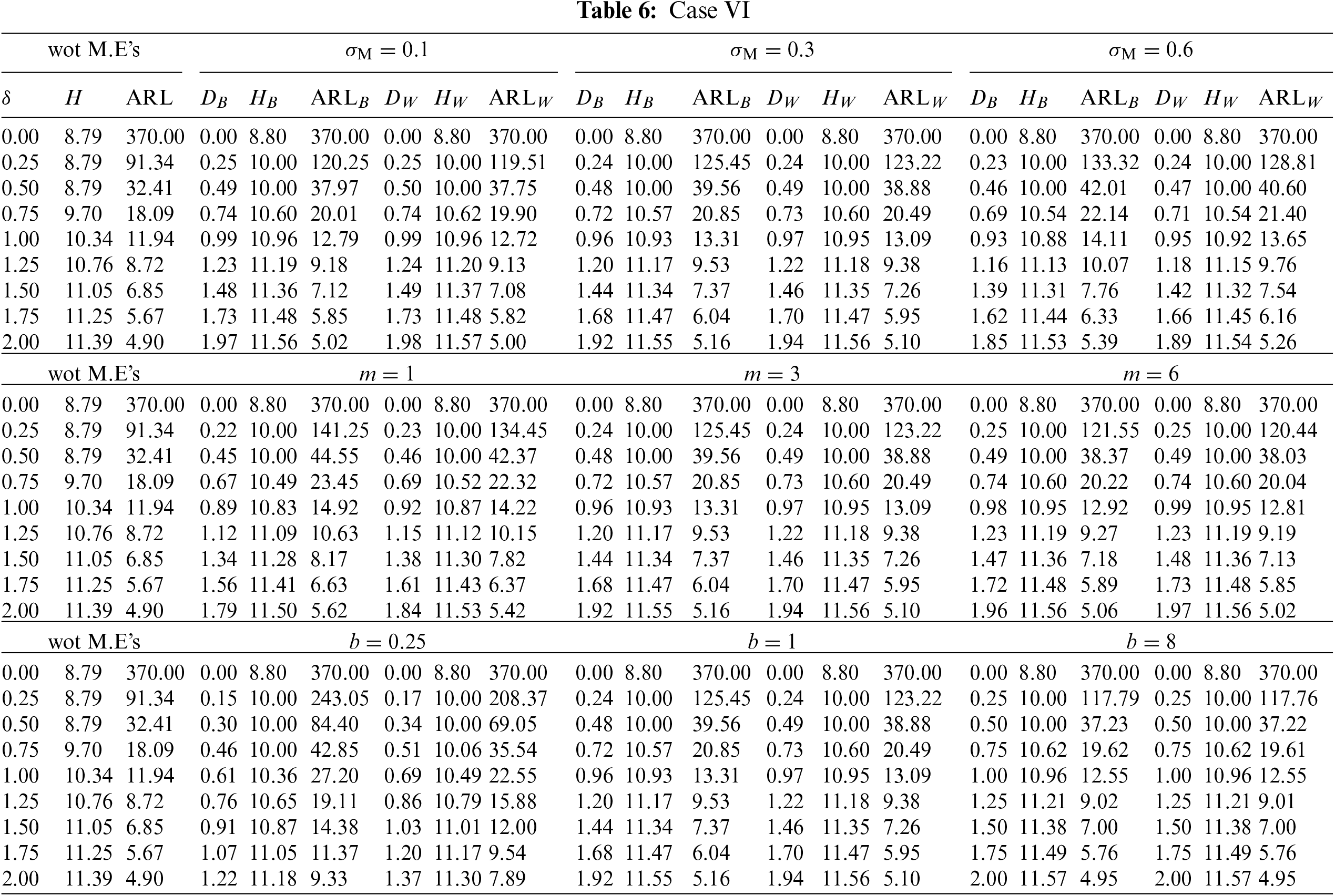
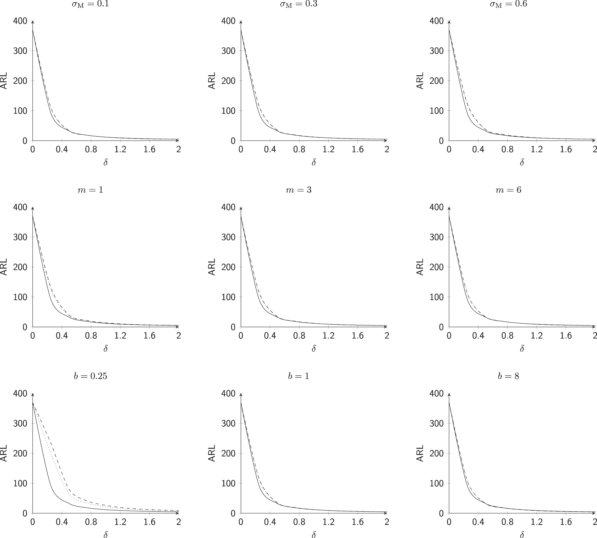
Figure 6:
5.7 Effect of Number of Variables p
This subsection investigates the effect of the number of variables involved p for all 6 cases mentioned above. The values of
For shifts
• For Case #1, when we increase the values of p, the
• For Case #2, when we increase the values of p, the
• For Case #3, when we increase the values of p, the
• For Case #4, when we increase the values of p, the
• For Case #5, when we increase the values of p, the
• For Case #6, when we increase the values of p, the
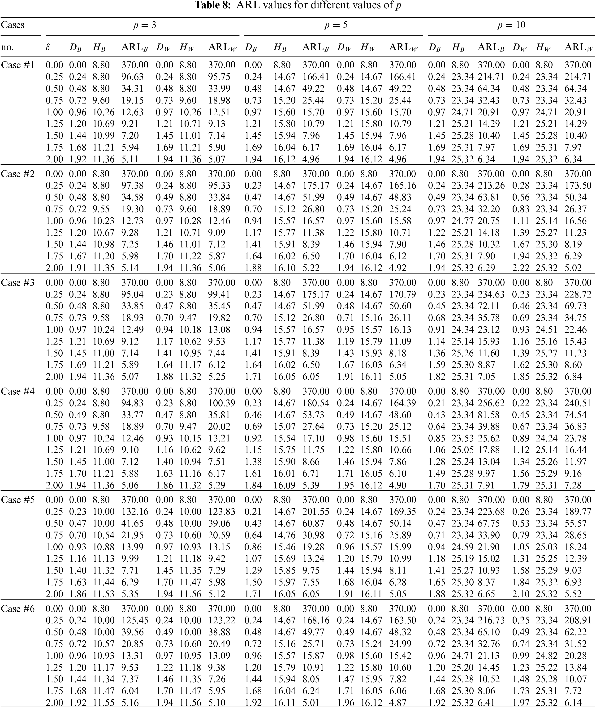
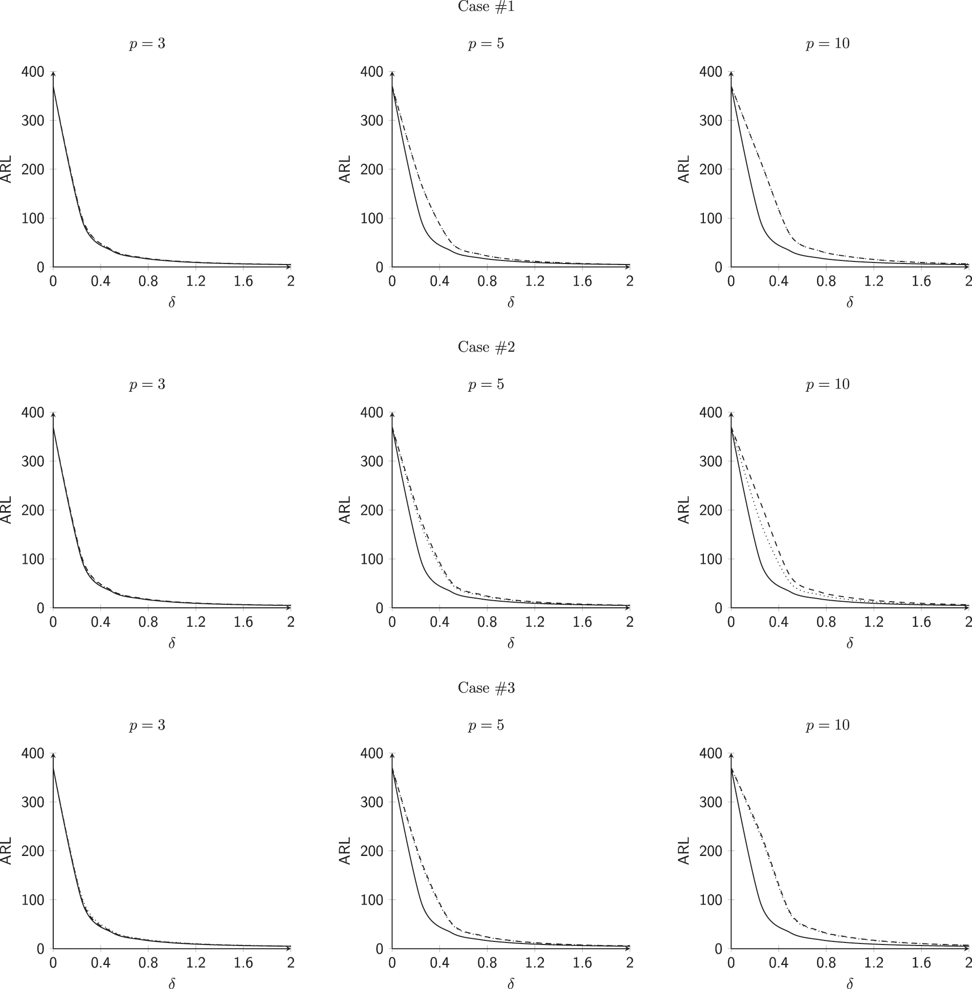
Figure 7:
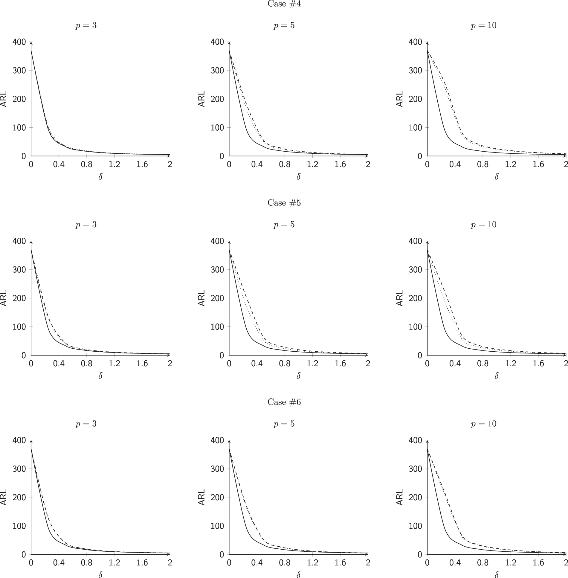
Figure 8:
6 Practical Implementation of the Proposal in the Manufacturing Scenario
For the proposal implementation, two illustrated examples have been incorporated in this study: one involving manufacturing uncoated aspirin tablets with the composition of aspirin, micro-crystalline cellulose, talcum powder and magnesium stearate and the other is the monitoring of machines that are responsible for the percentages of three components (whole-grain cereal, dried fruits, and nuts) in muesli production.
6.1 Proposal Implementation Related to Aspirin Manufacturing Process
Pharmaceutical manufacturing is the process of synthesizing pharmaceutical medications on a large scale as part of the pharmaceutical business. The medication production process may be divided into several unit activities, such as milling, granulation, coating, tablet pressing, etc. Here the authors simulated an example of a company producing uncoated aspirin tablets. The base parameters have been taken from [47]. According to Tiwari et al. [47], the composition of the tablet consists of 150 mg of aspirin, 60 mg of micro crystalline cellulose, 20 mg of talcum powder and magnesium stearate. The company wants to check the measuring unit in charge of measuring raw material (i.e., estimate a, b and
•
•
•
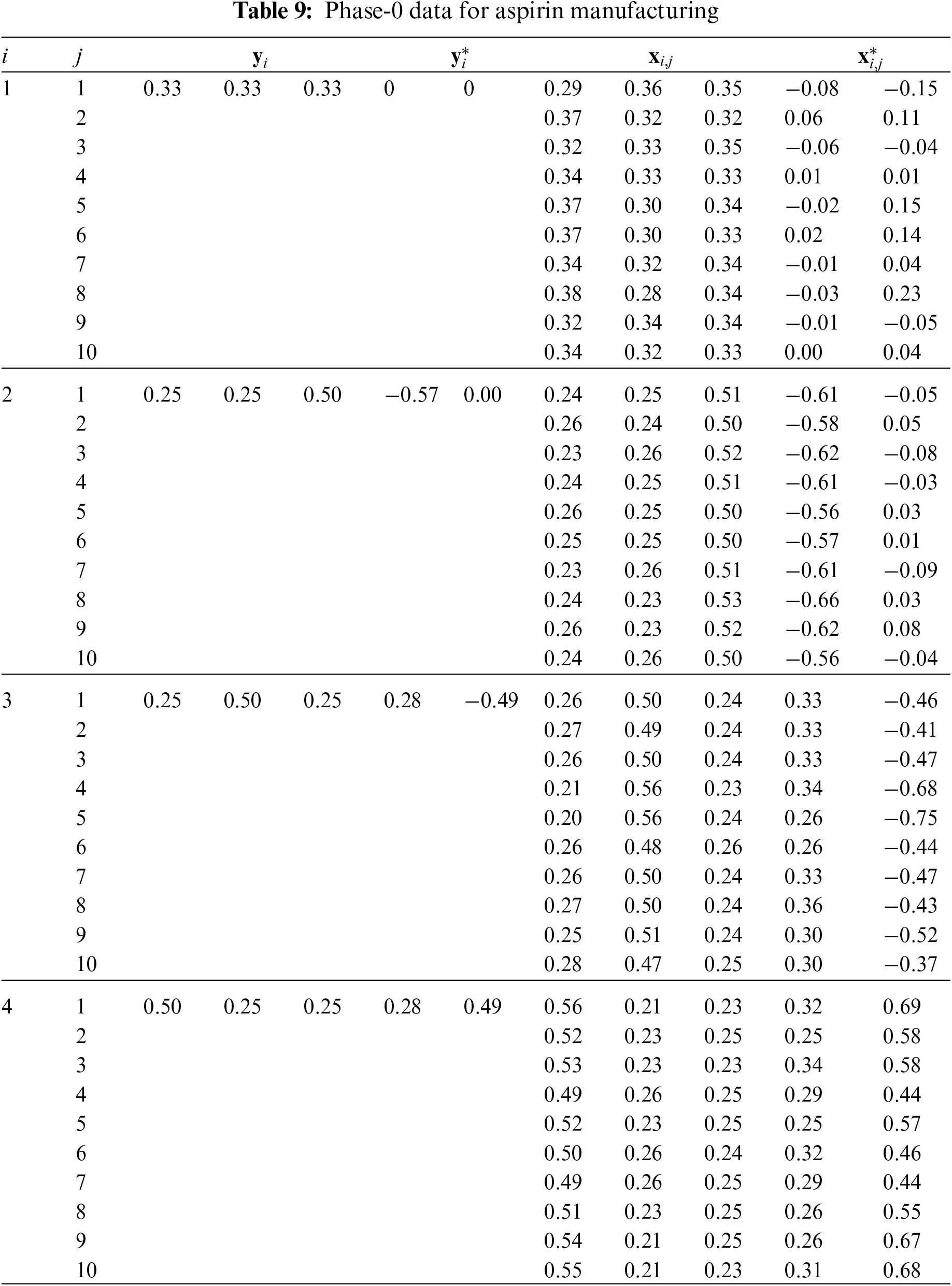
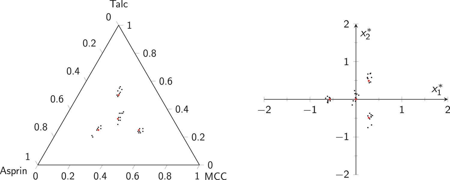
Figure 9: Data used to check machine:
The estimated values of
•
•
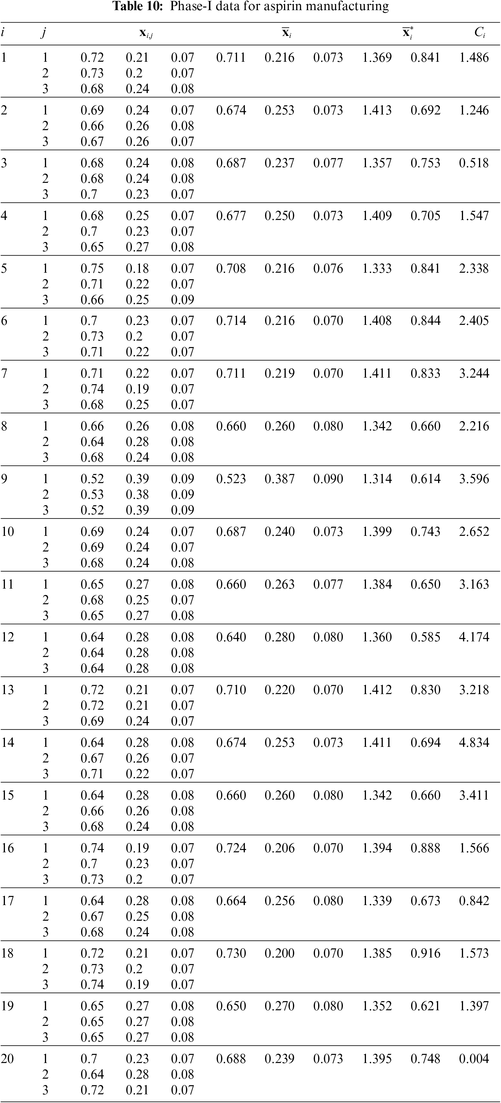
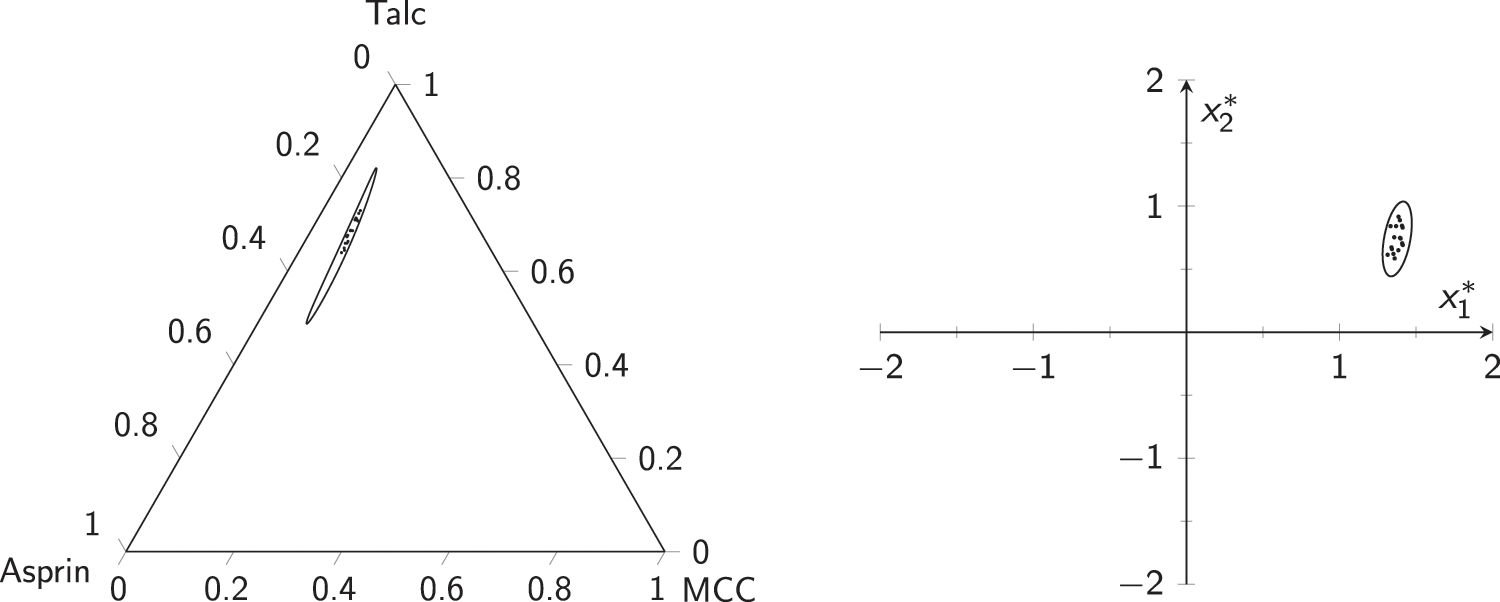
Figure 10: Phase-I data for aspirin example:
Using the above values, we can obtain
•
•
The results of the MCUSUM-CoDa charts are also presented in Table 10. Fig. 11 also shows the values of the MCUSUM-CoDa chart along with
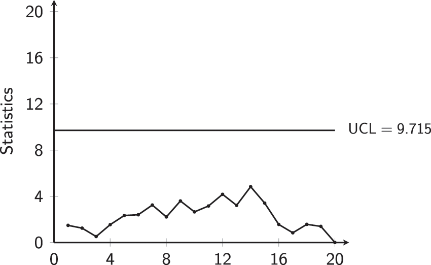
Figure 11: MCUSUM-CoDa chart for aspirin Phase-I data
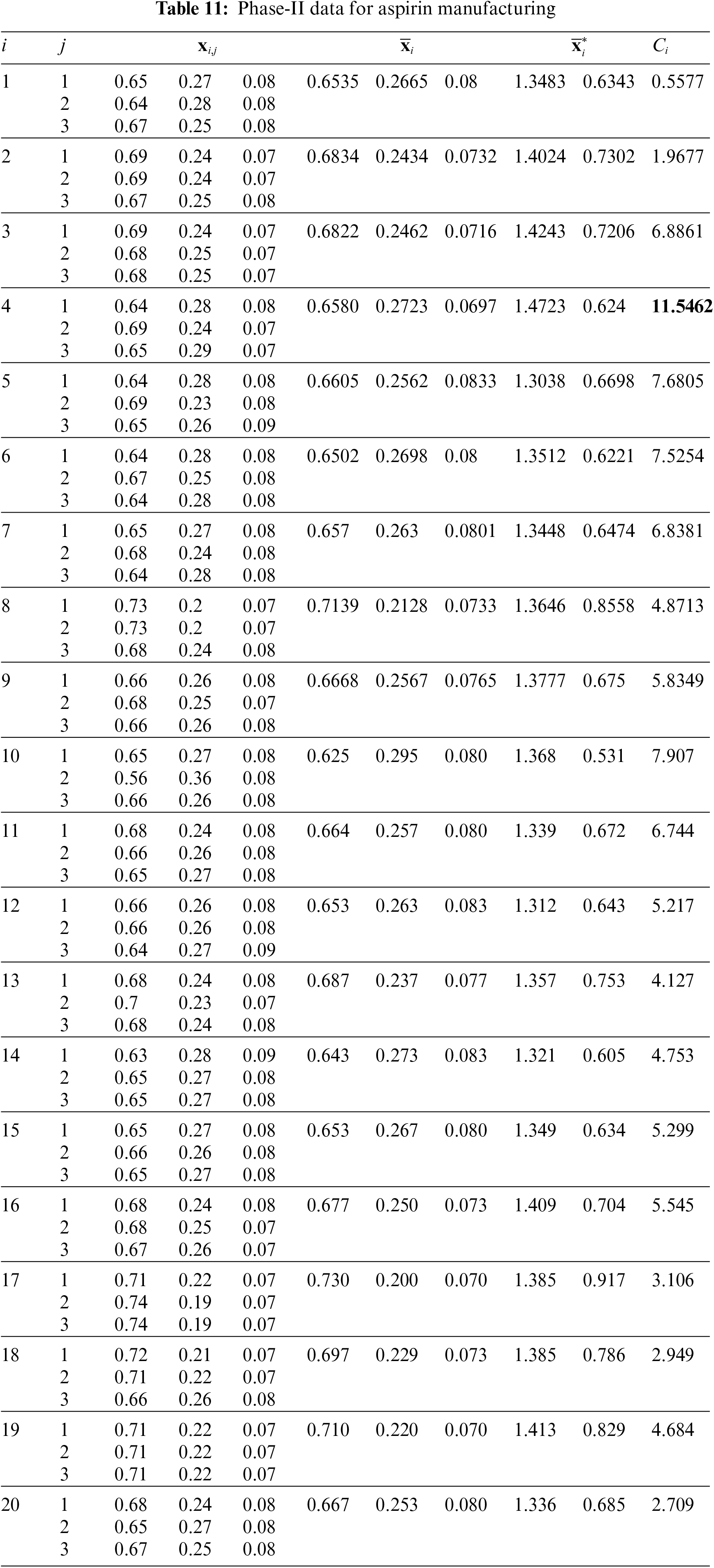
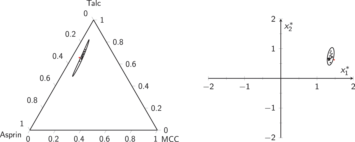
Figure 12: Phase-II data for aspirin example:
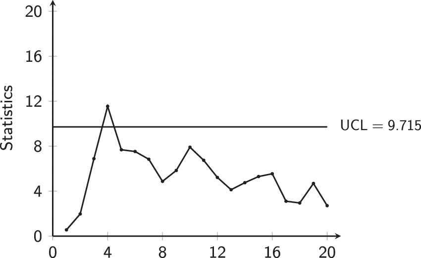
Figure 13: MCUSUM-CoDa chart for aspirin Phase-II data
6.2 Proposal Implementation Related to the Muesli Manufacturing Process
For the second example, the authors are using the same example used in [19] and [21] of a company that manufactures breakfast muesli with (A) 66 percent of cereals, (B) 24 percent dried fruits, and (C) 10 percent nuts in every 100 grams. The company has decided to begin by calibrating the measurement device used to determine the percentage of each component in the manufactured muesli (i.e., estimate
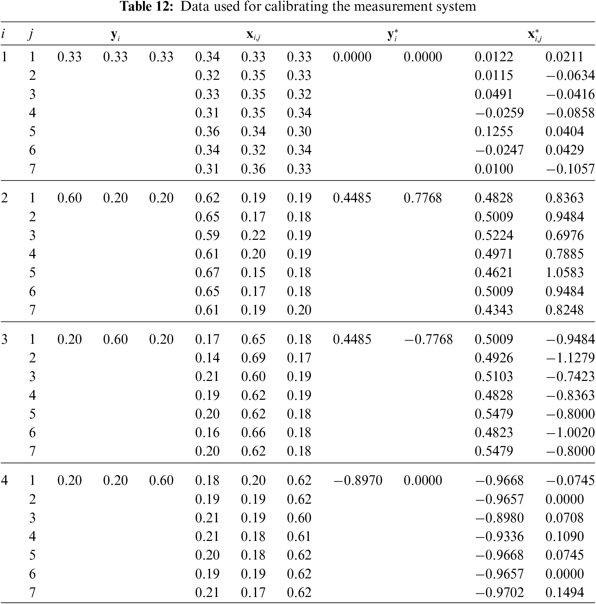
The following estimates are obtained using Table 12 with
•
•
•
To estimate the
•
•
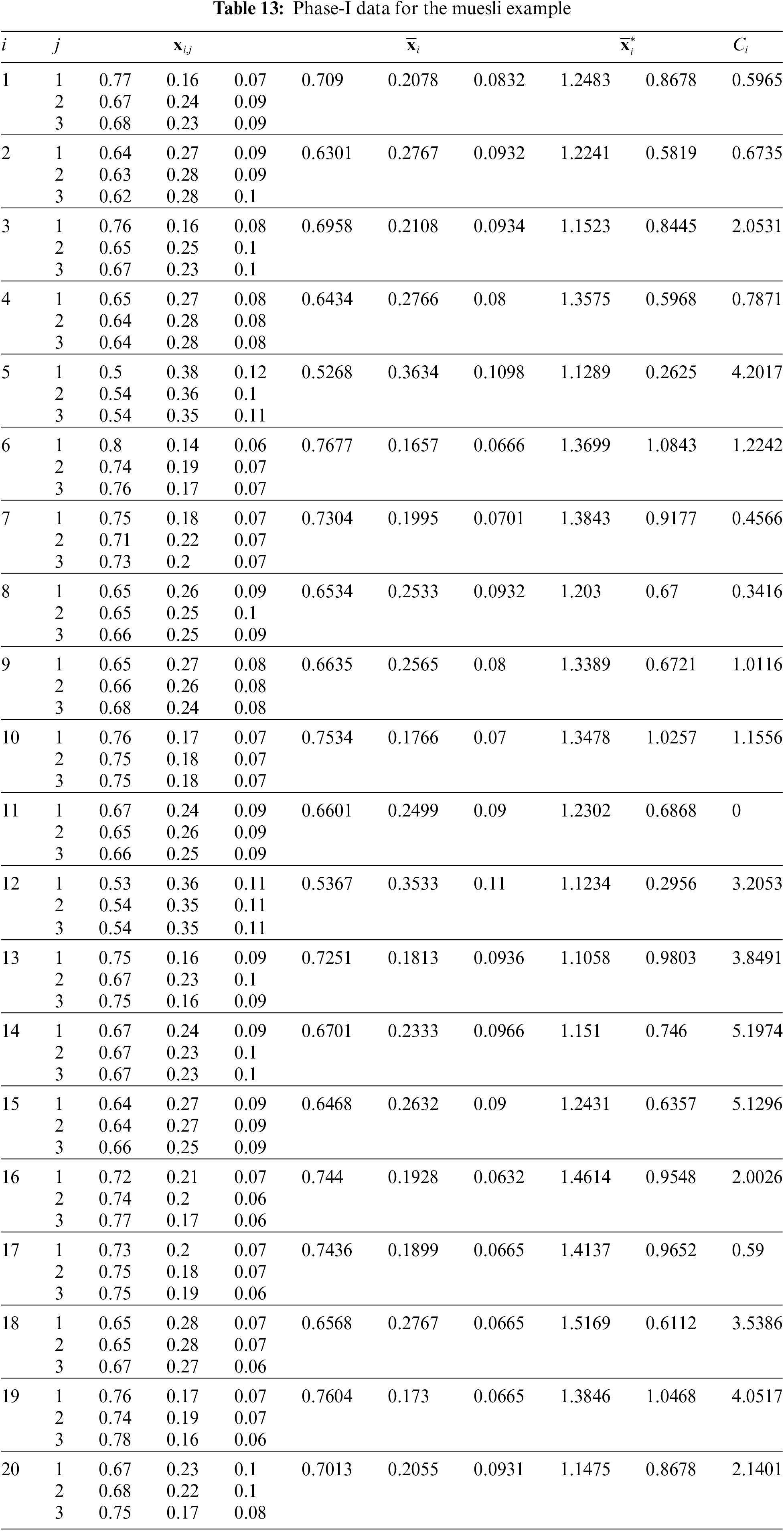
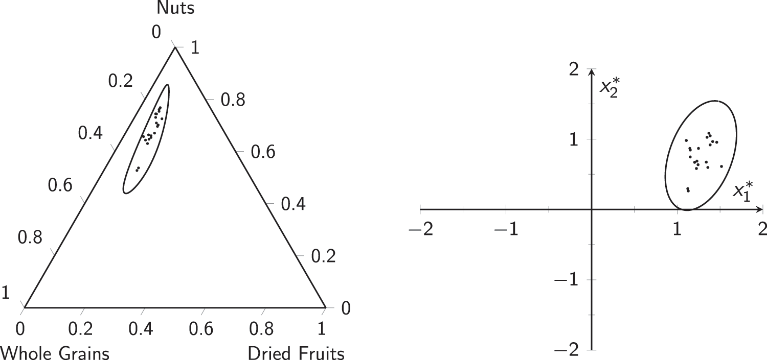
Figure 14: Phase-I data for the muesli example:
Then, using (10) and (11), we have
•
•
The authors have computed the MCUSUM-CoDa statistics
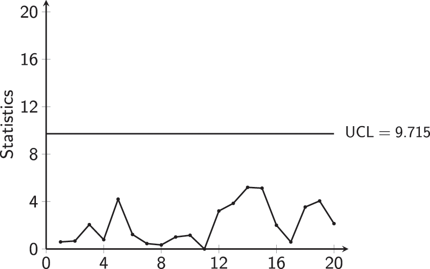
Figure 15: MCUSUM-CoDa CC for muesli Phase-I data
Concerning Phase-II,
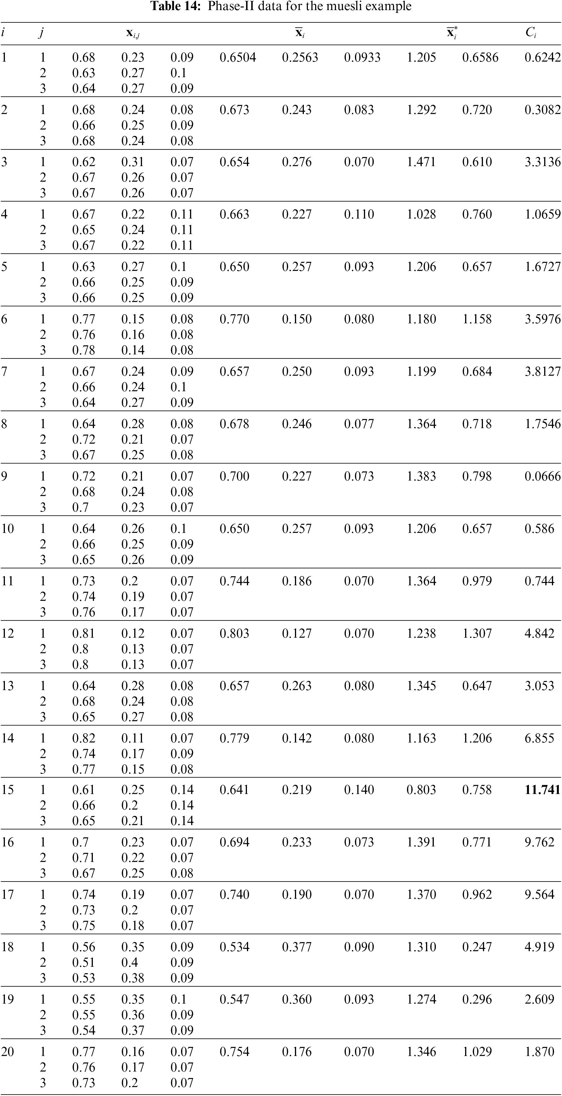

Figure 16: Phase-II data for the muesli example:
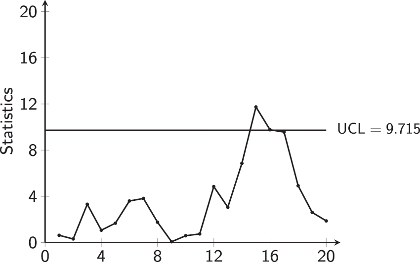
Figure 17: MCUSUM-CoDa CC for muesli Phase-II data
The process seems to be
The CCs are an effective statistical process monitoring tool frequently used to assess the stability of manufacturing processes. They monitor the industrial process by giving practitioners an early signal about an
Data and Code Availability Statement: All data, models, and codes supporting the results of this study are accessible on reasonable request from the corresponding author.
Ethics Approval: This manuscript has not been simultaneously submitted to more than one journal. So the proposed work is original and has not been published anywhere else in any form or language.
Consent to Participate and Publish: Consent was obtained from all authors for their participation in completing this manuscript and their consent to publish it.
Author’s Contribution: All the authors contributed to this paper.
Funding Statement: This work is supported by the National Natural Science Foundation of China (Grant No. 71802110); the Humanity and Social Science Foundation of the Ministry of Education of China (Grant No. 19YJA630061).
Conflicts of Interest: The authors declare that they have no conflicts of interest to report regarding the present study.
References
1. Fu, J. C., Shmueli, G., Chang, Y. M. (2003). A unified markov chain approach for computing the run length distribution in control charts with simple or compound rules. Statistics & Probability Letters, 65(4), 457–466. DOI 10.1016/j.spl.2003.10.004. [Google Scholar] [CrossRef]
2. Koutras, M. V., Sofikitou, E. M. (2017). A new bivariate semiparametric control chart based on order statistics and concomitants. Statistics & Probability Letters, 129, 340–347. DOI 10.1016/j.spl.2017.06.015. [Google Scholar] [CrossRef]
3. He, Y., Liu, F., Cui, J., Han, X., Zhao, Y. et al. (2019). Reliability-oriented design of integrated model of preventive maintenance and quality control policy with time-between-events control chart. Computers & Industrial Engineering, 129, 228–238. DOI 10.1016/j.cie.2019.01.046. [Google Scholar] [CrossRef]
4. Zaka, A., Akhter, A., Jabeen, R., Sanaullah, A. (2021). Control charts for the shape parameter of power function distribution under different classical estimators. Computer Modeling in Engineering & Sciences, 127(3), 1201–1223. DOI 10.32604/cmes.2021.014477. [Google Scholar] [CrossRef]
5. Liu, X., Khan, M., Rasheed, Z., Anwar, S., Arslan, M. (2022). New hybrid EWMA charts for efficient process dispersion monitoring with application in automobile industry. Computer Modelong in Engineering & Scinces, 131(2), 1171–1195. DOI 10.32604/cmes.2022.019199. [Google Scholar] [CrossRef]
6. Wang, J., Zhao, S., Liu, F., Ma, Z. (2022). Enhancing the effectiveness of trimethylchlorosilane purification process monitoring with variational autoencoder. Computer Modelong in Engineering & Scinces, 132(2), 531–552. DOI 10.32604/cmes.2022.019521. [Google Scholar] [CrossRef]
7. Nishimura, K., Matsuura, S., Suzuki, H. (2015). Multivariate EWMA control chart based on a variable selection using AIC for multivariate statistical process monitoring. Statistics & Probability Letters, 104, 7–13. DOI 10.1016/j.spl.2015.05.003. [Google Scholar] [CrossRef]
8. Gould, A. L. (2016). Control charts for monitoring accumulating adverse event count frequencies from single and multiple blinded trials. Statistics in Medicine, 35(30), 5561–5578. DOI 10.1002/sim.7073.. [Google Scholar] [CrossRef]
9. Moraes, D. A. O., Oliveira, F. L. P., Duczmal, L. H., Cruz, F. R. B. (2016). Comparing the inertial effect of MEWMA and multivariate sliding window schemes with confidence control charts. The International Journal of Advanced Manufacturing Technology, 84(5–8), 1457–1470. [Google Scholar]
10. Niaki, S. T. A., Ershadi, M. J., Malaki, M. (2010). Economic and economic-statistical designs of MEWMA control charts—A hybrid taguchi loss, markov chain, and genetic algorithm approach. The International Journal of Advanced Manufacturing Technology, 48(1), 283–296. DOI 10.1007/s00170-009-2288-0. [Google Scholar] [CrossRef]
11. Li, Q., Mukherjee, A., Song, Z., Zhang, J. (2021). Phase-II monitoring of exponentially distributed process based on type-II censored data for a possible shift in location Scale. Journal of Computational and Applied Mathematics, 389, 113315. [Google Scholar]
12. Ahmad, M. R., Ahmed, S. E. (2021). On the distribution of the T2 statistic, used in statistical process monitoring, for high-dimensional data. Statistics & Probability Letters, 168, 108919. [Google Scholar]
13. Aitchison, J. (1982). The statistical analysis of compositional data. Journal of the Royal Statistical Society. Series B (Methodological), 44(2), 139–177. [Google Scholar]
14. Aitchison, J. (2011). The statistical analysis of compositional data. In: Monographs on statistics and applied probability. Netherlands: Springer. [Google Scholar]
15. Pawlowsky-Glahn, V., Egozcue, J., Tolosana-Delgado, R. (2015). Modeling and analysis of compositional data. In: Statistics in practice. John Wiley & Sons. [Google Scholar]
16. Carreras-Sim, M., Coenders, G. (2020). Principal component analysis of financial statements: A compositional approach. Revista de Metodos Cuantitativos Para la Economia y la Empresa, 29, 18–37. [Google Scholar]
17. Morais, J., Thomas-Agnan, C., Simioni, M. (2018). Interpretation of explanatory variables impacts in compositional regression models. Austrian Journal of Statistics, 47(5), 1–25. [Google Scholar]
18. Egozcue, J., Pawlowsky-Glahn, V. (2019). Compositional data: The sample space and its structure. TEST, 28(3), 599–638. [Google Scholar]
19. Zaidi, F. S., Castagliola, P., Tran, K. P., Khoo, M. B. C. (2019). Performance of the hotelling T2 control chart for compositional data in the presence of measurement errors. Journal of Applied Statistics, 46(14), 2583–2602. [Google Scholar]
20. Tran, K. P., Castagliola, P., Celano, G., Khoo, M. B. C. (2018). Monitoring compositional data using multivariate exponentially weighted moving average scheme. Quality and Reliability Engineering International, 34(3), 391–402. [Google Scholar]
21. Zaidi, F. S., Castagliola, P., Tran, K. P., Khoo, M. B. C. (2020). Performance of the MEWMA-CoDa control chart in the presence of measurement errors. Quality and Reliability Engineering International, 36(7), 2411–2440. DOI 10.1002/qre.2705. [Google Scholar] [CrossRef]
22. Hawkins, D. M., Olwell, D. H. (1998). Cumulative sum charts and charting for quality improvement. In: Information science and statistics. New York: Springer-Verlag. [Google Scholar]
23. Knoth, S., Wittenberg, P., Gan, F. F. (2019). Risk-adjusted CUSUM charts under model error. Statistics in Medicine, 38(12), 2206–2218. DOI 10.1002/sim.8104. [Google Scholar] [CrossRef]
24. Shu, L., Jiang, W., Tsui, K. (2011). A comparison of weighted CUSUM procedures that account for monotone changes in population size. Statistics in Medicine, 30(7), 725–741. DOI 10.1002/sim.4122. [Google Scholar] [CrossRef]
25. Hotelling, H. (1947). Multivariate quality control, illustrated by the air testing of sample bombsights. In: Techniques of statistical analysis. New York: McGraw-Hill. [Google Scholar]
26. Healy, J. D. (1987). A note on multivariate CUSUM procedures. Technometrics, 29, 409–412. DOI 10.1080/00401706.1987.10488268. [Google Scholar] [CrossRef]
27. Alevizakos, V., Koukouvinos, C. (2020). A double progressive mean control chart for monitoring poisson observations. Journal of Computational and Applied Mathematics, 373, 112232. Numerical Analysis and Scientific Computation with Applications. DOI 10.1016/j.cam.2019.04.012. [Google Scholar] [CrossRef]
28. Alevizakos, V., Chatterjee, K., Koukouvinos, C. (2021). The triple moving average control chart. Journal of Computational and Applied Mathematics, 384, 113171. DOI 10.1016/j.cam.2020.113171. [Google Scholar] [CrossRef]
29. Nguyen, H. D., Tran, K. P., Tran, K. D. (2021). The effect of measurement errors on the performance of the exponentially weighted moving average control charts for the ratio of two normally distributed variables. European Journal of Operational Research, 293(1), 203–218. DOI 10.1016/j.ejor.2020.11.042. [Google Scholar] [CrossRef]
30. Bellotti, M., Qian, J., Reynaerts, D. (2020). Self-tuning breakthrough detection for EDM drilling micro holes. Journal of Manufacturing Processes, 57, 630–640. DOI 10.1016/j.jmapro.2020.07.031. [Google Scholar] [CrossRef]
31. Nguyen, H. D., Tran, K. P., Celano, G., Maravelakis, P. E., Castagliola, P. (2020). On the effect of the measurement error on shewhart t and EWMA T2 control charts. The International Journal of Advanced Manufacturing Technology, 107(9), 4317–4332. [Google Scholar]
32. Linna, K. W., Woodall, W. H. (2001). Effect of measurement error on shewhart control charts. Journal of Quality Technology, 33(2), 213–222. [Google Scholar]
33. Bennett, C. A. (1954). Effect of measurement error on chemical process control. Industrial Quality Control, 10(4), 17–20. [Google Scholar]
34. Montgomery, D. C., Keats, J. B., Runger, G. C., Messina, W. S. (1994). Integrating statistical process control and engineering process control. Journal of Quality Technology, 26(2), 79–87. [Google Scholar]
35. Maleki, M. R., Amiri, A., Castagliola, P. (2017). Measurement errors in statistical process monitoring: A literature review. Computers & Industrial Engineering, 103, 316–329. [Google Scholar]
36. Maravelakis, P., Panaretos, J., Psarakis, S. (2004). EWMA chart and measurement error. Journal of Applied Statistics, 31(4), 445–455. [Google Scholar]
37. Hu, X., Castagliola, P., Sun, J., Khoo, M. B. C. (2016). Effect of measurement errors on the VSI X chart. European Journal of Industrial Engineering, 10(2), 224–242. [Google Scholar]
38. Maleki, M. R., Salmasnia, A., Yarmohammadi, S. (2022). The performance of triple sampling
39. Zaka, A., Naveed, M., Jabeen, R. (2022). Performance of attribute control charts for monitoring the shape parameter of modified power function distribution in the presence of measurement error. Quality and Reliability Engineering International, 38(2), 1060–1073. [Google Scholar]
40. Li, Q., Yang, J., Huang, S., Zhao, Y. (2022). Generally weighted moving average control chart for monitoring two-parameter exponential distribution with measurement errors. Computers & Industrial Engineering, 165, 107902. [Google Scholar]
41. Yousefi, S., Maleki, M., Salmasnia, A., Anbohi, M. K. M. (2022). Performance of multivariate homogeneously weighted moving average chart for monitoring the process mean in the presence of measurement errors. Journal of Advanced Manufacturing Systems. DOI 10.1142/S0219686723500026. [Google Scholar] [CrossRef]
42. Crosier, R. B. (1986). A new two-sided cumulative sum quality control scheme. Technometrics, 28, 187–194. DOI 10.1080/00401706.1986.10488126. [Google Scholar] [CrossRef]
43. Imran, M., Sun, J., Zaidi, F. S., Abbas, Z., Nazir, H. Z. (2022). Multivariate cumulative sum control chart for compositional data with known and estimated process parameters. Quality and Reliability Engineering International, 38(5), 2691–2714. DOI 10.1002/qre.3099. [Google Scholar] [CrossRef]
44. Lowry, C. A., Woodall, W. H., Champ, C. W., Rigdon, S. E. (1992). A multivariate exponentially weighted moving average control chart. Technometrics, 34(1), 46–53. DOI 10.2307/1269551. [Google Scholar] [CrossRef]
45. Gnanadesikan, M., Gupta, S. S. (1970). A selection procedure for multivariate normal distributions in terms of the generalized variances. Technometrics, 12(1), 103–117. DOI 10.1080/00401706.1970.10488638. [Google Scholar] [CrossRef]
46. Montgomery, D. C. (2007). Introduction to statistical quality control. 4th edition. Hoboken, New Jersey: John Wily & Sons. [Google Scholar]
47. Tiwari, S., Wadher, S. J., Yemul, O. S. (2018). Formulation and evaluation of enteric coated aspirin tablet by using bio epoxy resin as coating material. Journal of Pharmaceutics & Drug Delivery Research, 7(2), 4668–4672. DOI 10.4172/2325-9604.1000179. [Google Scholar] [CrossRef]
48. Mardia, K., Kent, J., Bibby, J. (1979). Multivariate analysis. Probability and Mathematical Statistics, London: Academic Press. [Google Scholar]
Appendix A
Let
where
Then, an estimation of
Appendix B
Let
subject to the constraint
As presented in [48] (Theorem A.9.2 page no. 479), one can prove that if
and
Similarly
Following Mardia 1979, the author also used c = 1.
Appendix C
The Scilab Codes for ARL, when
ARL0 = 370;
d1 = 0.25; d2 = 0.5; d3 = 0.75; d4 = 1; d5 = 1.25; d6 = 1.5; d7 = 1.75; d8 = 2;
p = 3;
b = 1;
mm = 3;
S = [3, 0;0, 3];
SM = 0.3 * eye(p−1, p−1);
b2 = b * b
AA = b2 * inv(b2 * S + SM/mm)
BB = inv(S)
invBB = S [eve, eva] = spec(invBB * AA) if eva(1, 1) < eva(2, 2) then lam1 = eva(1, 1) lam2 = eva(2, 2) v1 = eve(:, 1)
vp = eve(:, 2)
else
lam1 = eva(2, 2)
lam2 = eva(1, 1)
v1 = eve(:, 2)
vp =eve(:, 1)
end
m1 = 30
m2 = 30
dmi1 = d1 * lam1 dma1 = d1 * lam2
dmi2 = d2 * lam1 dma2 = d2 * lam2
dmi3 = d3 * lam1 dma3 = d3 * lam2
dmi4 = d4 * lam1 dma4 = d4 * lam2
dmi5 = d5 * lam1 dma5 = d5 * lam2
dmi6 = d6 * lam1 dma6 = d6 * lam2
dmi7 = d7 * lam1 dma7 = d7 * lam2
dmi8 = d8 * lam1 dma8 = d8 * lam2
[r21,H21,ARL21,SDRL21] = optMEWMAUTM(m1, m2, p−1,ARL0, dmi1)
Z21 = [dmi1;r21;H21;ARL21] [r31,H31,ARL31,SDRL31] = optMEWMAUTM(m1, m2,
p−1,ARL0, dma1)
Z31 = [dma1;r31;H31;ARL31]
disp(Z21) disp(Z31)
[r22,H22,ARL22,SDRL22] = optMEWMAUTM(m1, m2, p−1,ARL0, dmi2)
Z22 = [dmi2;r22;H22;ARL22] [r32,H32,ARL32,SDRL32] = optMEWMAUTM(m1, m2,
p−1,ARL0, dma2)
Z32 = [dma2;r32;H32;ARL32]
disp(Z22) disp(Z32) [r23,H23,ARL23,SDRL23] = optMEWMAUTM(m1, m2, p−1,ARL0, dmi3)
Z23 = [dmi3;r23;H23;ARL23] [r33,H33,ARL33,SDRL33] = optMEWMAUTM(m1, m2,p−1,ARL0, dma3)
Z33 = [dma3;r33;H33;ARL33]
disp(Z23) disp(Z33)
[r24,H24,ARL24,SDRL24] = optMEWMAUTM(m1, m2, p−1,ARL0, dmi4)
Z24 = [dmi4;r24;H24;ARL24] [r34,H34,ARL34,SDRL34] = optMEWMAUTM(m1, m2,
p−1,ARL0, dma4)
Z34 = [dma4;r34;H34;ARL34]
disp(Z24) disp(Z34)
[r25,H25,ARL25,SDRL25] = optMEWMAUTM(m1, m2, p−1,ARL0, dmi5)
Z25 = [dmi5;r25;H25;ARL25] [r35,H35,ARL35,SDRL35] = optMEWMAUTM(m1, m2,
p−1,ARL0, dma5)
Z35 = [dma5;r35;H35;ARL35]
disp(Z25) disp(Z35)
[r26,H26,ARL26,SDRL26] = optMEWMAUT(m1, m2, p−1,ARL0, dmi6)
Z26 = [dmi6;r26;H26;ARL26] [r36,H36,ARL36,SDRL36] = optMEWMAUT(m1, m2, p−1,ARL0, dma6)
Z36 = [dma6;r36;H36;ARL36]
disp(Z26) disp(Z36)
[r27,H27,ARL27,SDRL27] = optMEWMAUTM(m1, m2, p−1,ARL0, dmi7)
Z27 = [dmi7;r27;H27;ARL27] [r37,H37,ARL37,SDRL37] = optMEWMAUTM(m1, m2,
p−1,ARL0, dma7)
Z37 = [dma7;r37;H37;ARL37]
disp(Z27) disp(Z37)
[r28,H28,ARL28,SDRL28] = optMEWMAUTM(m1, m2, p−1,ARL0, dmi8)
Z28 = [dmi8;r28;H28;ARL28] [r38,H38,ARL38,SDRL38] = optMEWMAUTM(m1, m2,
p−1,ARL0, dma8)
Z38 = [dma8;r38;H38;ARL38]
disp(Z28) disp(Z38)
Where the base function “optCUSUMUTM” to find the ARL is given below,
//———————————— function [Q0, q0] = QCUSUM0M(H, k, p) //————————–
// in control [argout, argin] = argn() if (argin<3)|(argin>4) error(“incorrect number of arguments”) end if H<=0 error(“argument “H” must be > 0”)
end if k<=0 error(“argument “k” must be > 0”)
end if p<=0 error(“argument “p” must be > 0”)
end
UCL = H
m = 100
g = 2 * UCL/(2 * m + 1)
Q0 = ones(m + 1, m + 1)
t = [0:1:m]
down = repmat(downi, 1, m + 1)
C = repmat(c, m, 1)
Q02 = cdfchn(“PQ”, up, p * ones(m, m + 1),C)-cdfchn(“PQ”, down, p * ones(m, m + 1),C)
Q0 = [Q01;Q02]’
q0 = zeros(m + 1, 1)
q0(1) = 1
endfunction
//————————— function [ARL,SDRL] = rlCUSUM0M(H, k, p) //—————————
// in-control ARL [argout, argin] = argn() if (argin<3)|(argin>4) error(”incorrect number of arguments”) end if H<=0 error(“argument “H” must be > 0”)
end if k<=0 error(“argument “k” must be > 0”)
end if p<=0 error(“argument “p” must be > 0”)
end [Q0, q0] = QCUSUM0(H, k, p)
W = inv(eye(Q0)-Q0)
Z = q0’ * W
ARL = sum(Z)
if argout == 2
Z = Z * W * Q0
//—————————- function [Q, q] = QCUSUM1M(H, m1, m2, k, p, delta) //——————
//Out-of-control [argout, argin] = argn() if (argin<5)|(argin>6) error(“incorrect number of arguments”) end if H<=0 error(“argument “H” must be > 0”)
end if k<=0 error(“argument “k” must be > 0”)
end if p<=0 error(“argument “p” must be > 0”)
end
UCL = H;
g1 = 2 * UCL/(2 * m1 + 1);
Q1 = ones(2 * m1 + 1, 2 * m1 + 1);
t1 = [1:1:2 * m1 + 1];
c1 = -UCL + (t1–0.5) * g1;
C1 = repmat(c1, 2 * m1 + 1, 1);
tt1 = [1:1:2 * m1 + 1]’;
Tt1 = repmat(tt1, 1, 2 * m1 + 1);
up1 = (-UCL + Tt1 * g1−(1−k) * C1)/k−delta;
down1 = (−UCL + (Tt1–1) * g1−(1−k) * C1)/k-delta;
Q11 = cdfnor(“PQ”, up1, 0 * ones(C1), 1 * ones(C1))-cdfnor(“PQ”, down1, 0 * ones(C1), 1 * ones(C1)); Q1 = Q11’;
g2 = 2 * UCL/(2 * m2 + 1);
Q2 = ones(m2 + 1, m2 + 1);
t2 = [0:1:m2];
Q(:, counter) = 0;
Q(counter,:) = 0;
end
counter = counter + 1;
end
end
q = zeros((2 * m1 + 1) * (m2 + 1), 1)
start = m1 * (m2 + 1) + 1
q(start) = 1
endfunction
//——————— function [ARL,SDRL] = rlCUSUM1M(H, m1, m2, k, p, delta) //—————
//Out-of-Control ARL [argout, argin] = argn() if (argin<5)|(argin>6) error(“incorrect number of arguments”) end if H<=0 error(“argument “H” must be > 0”)
end if k<=0 error(“argument “k” must be > 0”)
end if p<=0 error(“argument “p” must be > 0”)
end [Q, q] = QCUSUM1M(H, m1, m2, k, p, delta)
W = inv(eye(Q)-Q)
Z = q’ * W
ARL = sum(Z)
if argout == 2
Z = Z * W * Q
end endfunction
//——————————- function f = HCUSUMM(H, k, arl0, p) //——————————-
// function of H
if (H<=0)
f = else
ARL = rlCUSUM0M(H, k, p)
f = (arl0-ARL)
end endfunction
//————- function [H,ARL,SDRL] = optMEWMAUTM(m1, m2, p, arl0, delta) //————-
// Final ARL with optimal H [argout, argin] = argn()
if argin = 5 error(”incorrect number of arguments”)
end
lines(0)
k = 0.5
H0 = 7
H = simplexolve(H0,HCUSUMM, list(k, arl0, p), tol = 1e-4); [ARL,SDRL] = rlCUSUM1M(H, m1, m2, k, p, delta)
endfunction
Cite This Article
 Copyright © 2023 The Author(s). Published by Tech Science Press.
This work is licensed under a Creative Commons Attribution 4.0 International License , which permits unrestricted use, distribution, and reproduction in any medium, provided the original work is properly cited.
 Downloads
 Citation Tools